


1. Introduction
The major Indian rivers, i.e. the Indus, Ganga and Brahmputra and their numerous tributaries, originate from the high-altitude regions of the Himalaya. This region is normally covered by seasonal snow cover during winter. Snowmelt during summer forms an important component of stream runoff. Some estimates suggest annual runoff from snow and glacier melt is almost 30–50% (Reference Agarwal, Kumar and DasAgarwal and others, 1983). The snow and glacier melt is crucial, as this is available during critical summer months. Therefore, monitoring of seasonal snow cover is important to assess the availability of water in north Indian rivers. The seasonal snowmelt is significantly influenced by changes in atmospheric temperature and it can influence the distribution of stream runoff (Reference Kulkarni, Mathur, Rathore, Alex, Thakur and KumarKulkarni and others, 2002).
The Earth has experienced repeated cycles of glaciations (Reference PricePrice, 1973; Reference RuddimanRuddiman, 2005). However, this natural cycle may have altered due to the greenhouse effect, caused by man-made changes in the Earth’s environment. The Earth has experienced an increase in global temperature by 0.6 ± 0.2°C since 1900 (Reference Lozan, Grassl and HupferLozan and others, 2001). In addition, recent developments in climate modeling suggest that existing greenhouse gases and aerosols in the atmosphere have led to the Earth absorbing 0.85 ± 0.15 Wm−2 more energy than it emits to space (Reference HansenHansen and others, 2005). This means additional global warming of about 0.6°C without further change in atmospheric composition (Reference HansenHansen and others, 2005). The Fourth Assessment Report of the Intergovernmental Panel on Climate Change (IPCC) Working Group I suggests a temperature rise of 1.8–4.0°C up to 2090–99 relative to 1980–99, depending upon different emission scenarios of the Special Report on Emissions Scenarios. This can influence the distribution of seasonal snow cover. In the Northern Hemisphere, snow-cover observation from satellite data over the 1966–2005 period decreased every month, except during November and December, with a step-wise drop of 5% in the annual mean in the late 1980s (Reference Lemke and SolomonLemke and others, 2007). In addition, the same report also suggests that the duration of seasonal snow cover in the Himalayan region will shorten and snow cover will melt earlier than today, causing a shortage of water in spring and early summer (Reference Lemke and SolomonLemke and others, 2007). In the Baspa and Beas river basins in the Himalaya, snowmelt and retreat of snow cover were observed throughout winter and also at altitudes up to 4800 m (Reference Kulkarni, Mathur, Rathore, Alex, Thakur and KumarKulkarni and others, 2002). This change in snowmelt pattern can influence the runoff of all streams originating from the higher Himalaya. However, in the Himalaya, longterm records of snow-cover observations are not available. Depending upon area–altitude distribution and location of the basin in the Himalayan region, each basin is likely to respond differently to climate change.
Mapping and monitoring seasonal snow cover using field methods is normally very difficult in mountainous terrain like the Himalaya, so remote-sensing techniques have been extensively used for snow-cover monitoring. Snow-cover monitoring using satellite images began in April 1960 using the TIROS-1 satellite (Reference Singer and PophamSinger and Popham, 1963). Since then, numerous satellites (e.g. GOES, Meteosat, NOAA, MODIS and Resourcesat) have been used successfully for snow mapping (Reference Hall, Riggs and SalomonsonHall and others 1995; Reference Kulkarni, Singh, Mathur and MishraKulkarni and others 2006; Reference De Ruyter de Wildt, Seiz and Gruende Ruyter de Wildt and others, 2007). In this investigation, the Advanced Wide Field Sensor (AWiFS) of the RESOURCESAT-1 satellite was used to monitor seasonal snow cover in the western and central Himalayan basins Ganga, Satluj, Chenab and Indus. These basins were subdivided into 28 sub-basins. The locations and names of the sub-basins are given in Figure 1 and Table 1, respectively.
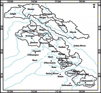
Fig. 1. Location map of 28 sub-basins in the western Himalaya.
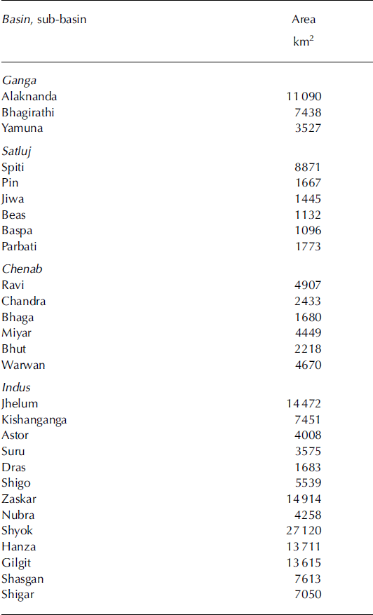
Table 1. Major river basins and sub-basins
2. Data
AWiFS data covering an areal extent of 183 405 km2 at an interval of 5 days were used. Approximately 1500 AWiFS scenes from October to June of the years 2004/05, 2005/06 and 2006/07 were analyzed in this investigation. Snow-cover monitoring was not carried out after June due to cloud cover in the monsoon season. The sensor specifications of AWiFS are given by Reference Kulkarni, Singh, Mathur and MishraKulkarni and others (2006). Altitude information of the Shuttle Radar Topography Mission (SRTM) was used. The digital elevation model (DEM) product with spatial resolution of 3″ with a vertical root-mean-square error (RMSE) of 16m was used (Reference Rabus, Eineder, Roth and BamlerRabus and others, 2003).
3. Methodology
Initially, a master template was generated using control points from 1 :250 000 scale maps and then basin boundaries were delineated using a drainage map. The master template was used for registration of all satellite data. Then an algorithm based on the normalized-difference snow index (NDSI) was used to map snow cover (Reference Kulkarni, Singh, Mathur and MishraKulkarni and others 2006). NDSI was calculated using the ratio of the green (band 2) and shortwave infrared (SWIR; band 5) channels of the AWiFS sensor. NDSI is established using the following method:
To estimate NDSI, digital numbers (DNs) were converted into top-of-atmosphere reflectance. This involves conversion of DNs into the radiance values, known as sensor calibration, and then reflectance was estimated. The various parameters (e.g. maximum and minimum radiances, mean solar exoatmospheric spectral irradiances in the satellite sensor bands, satellite data acquisition time, solar declination, solar zenith and solar azimuth angles and mean Earth–Sun distance) were used to estimate reflectance (Reference Markham and BarkerMarkham and Barker, 1987; Reference Srinivasulu and KulkarniSrinivasulu and Kulkarni, 2004). Sensitivity analysis has shown that a NDSI value of 0.4 can be taken as a threshold to differentiate between snow and non-snow pixels. Exoatmospheric reflectance of bands 2 and 5 of the AWiFS sensor was used to compute the NDSI, and no atmospheric correction has been applied at present. Field investigations suggest that NDSI values are independent of illumination conditions, i.e. snow/non-snow pixels can be identified under different slopes and orientations, even under mountain shadow region (Reference Kulkarni, Singh, Mathur and MishraKulkarni and others, 2006).
Snow extent is estimated at intervals of 5 or 10 days, depending upon the availability of AWiFS data. Cloud over snow-covered region is a critical issue and can introduce significant errors. In (10 d)−1 product, three scenes are analyzed, if available. For example, for 10 March, product data of 5, 10 and 15 March were used. If any pixel was identified as snow on any one date, then it was classified as snow on final product. If three consecutive scenes are not available, then all available scenes in the 10day window were used in the analysis. This will be used to generate basin-wise (10 d)−1 product information and is expected to have at least one scene under cloud-free conditions for each pixel. In the present algorithm, water bodies are marked in the pre-winter season and masked in the final products during winter, as separation of snow and water is difficult using reflectance, due to mountain shadow.
SRTM data were used to generate contours at intervals of 500 or 1000m and then the area within each contour was estimated using the Geographic Information System technique. The area–altitude information was generated for all 28 sub-basins in the western and central Himalaya, and then mosaic was prepared to estimate area–altitude distribution for the study area. A combination of area–altitude distribution and snow map was used to estimate snow-cover distribution in each altitude zone for the individual basin and for the western and central Himalaya. Area–altitude distribution was also used to develop a hypsographic curve. This curve gives the areal extent of the study area below any given altitude. The hypsographic curve and snow-free area of the western and central Himalaya in each month was used to estimate monthly snow-line elevation.
4. Validation of Ndsi Algorithm Using Awifs
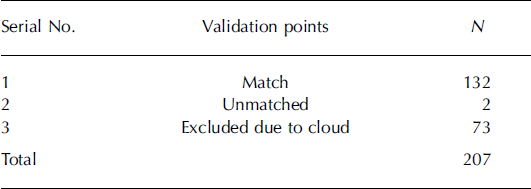
Validation of the snow-cover mapping algorithm was carried out in Beas basin. Three locations were selected in Beas basin, and respective GPS locations were taken. A total of 69 AWiFS scenes were processed from December 2003 to October 2005. Each pixel was classified as completely snow-covered or snow-free. Out of 207 points, 73 were excluded due to the presence of ice cloud, which gives a signature similar to snow, and removed from the final validation exercise. Out of 134 points, 132 were correctly classified as snow/non-snow pixels (Table 2).
Table 2. Validation exercise using NDSI
In the second method, a geographical area around Beas basin was selected. AWiFS data of 1 September 2005 were used to classify the region into three classes as snow or ice, barren land, or soil and vegetation, when most of the area was snow-free. The ISODATA technique was used for classification. Then, to estimate the accuracy of snow products, satellite imagery of 26 February 2006 was selected, when the region was completely snow-covered. This assessment was made based on field observations on snowfall. The snow product suggests an error less than 1% for all three classes.
However, this error will significantly increase if the region is covered by ice clouds. Ice clouds often have a signature similar to snow, and corresponding pixels can be misclassified. This can add significant error to the final results. For example, in Parbati river basin in Himachal Pradesh in 2004/05, in 18 out of 58 scenes clouds were misclassified as snow. Due to lack of thermal band in AWiFS, the present algorithm has little potential to correct this problem. Therefore, satellite data were checked manually after geocoding, and scenes were rejected if ice clouds were observed in the basin area. Manual separation between snow and ice cloud is possible due to textural differences (Reference Kulkarni and RathoreKulkarni and Rathore, 2003).
5. Results and Discussions
Snow-cover extent of 28 basins was mapped (Fig. 2) and then combined to estimate snow-cover extent for the central and western Himalaya. The changes in areal extent of snow cover for the central and western Himalaya are plotted in Figure 3. In the winter of 2004/05, for the period between October and mid-December, snow cover was <50%, increasing to 82% by the end of January. Snow extent remained >80% until the beginning of April. Snow-cover retreat then proceeded until the end of June, when relative snow-cover extent was only 37%. Similar trends were observed for 2005/06 and 2006/07.

Fig. 2. (10 d)−1 snow-cover product of Ravi basin.
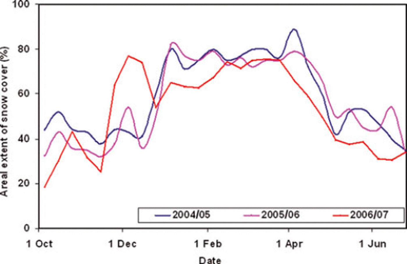
Fig. 3. Changes in areal extent of snow cover in relation to total area from October to June for 2004/05, 2005/06 and 2006/07 at an interval of 10 days for the western and central Himalayan region.
Area–altitude distribution can also influence snow accumulation and ablation. The study area is mostly located between 4000 and 5000 m a.s.l., with a small area above 6000 ma.s.l. (Figs 4 and 5). The hypsographic curve (Fig. 5) in combination with (10 d)−1 snow-cover product was used to estimate lowest snow-line altitude at an interval of 10 days for the three years between October and June (Fig. 6). The lowest snow-line altitude in the winter of 2004/05 was observed at 2480 m on 25 February 2005. Snow-line altitude remained below 3000m between 5 January 2005 and 15 April 2005. The highest snow-line altitude was estimated at 4620 m by the end of June. Three (10 d)−1 snow-cover products were used to estimate mean monthly snow-cover extent. Mean monthly snow cover and hypsographic curve were used to estimate mean monthly snow-line altitude (Table 3). The lowest mean monthly snow line in 2004/05 was lower than in the other two years, due to lower snowfall in 2005/06 and 2006/07. The lowest and highest mean monthly snow lines during the three years were observed for February and October, respectively.
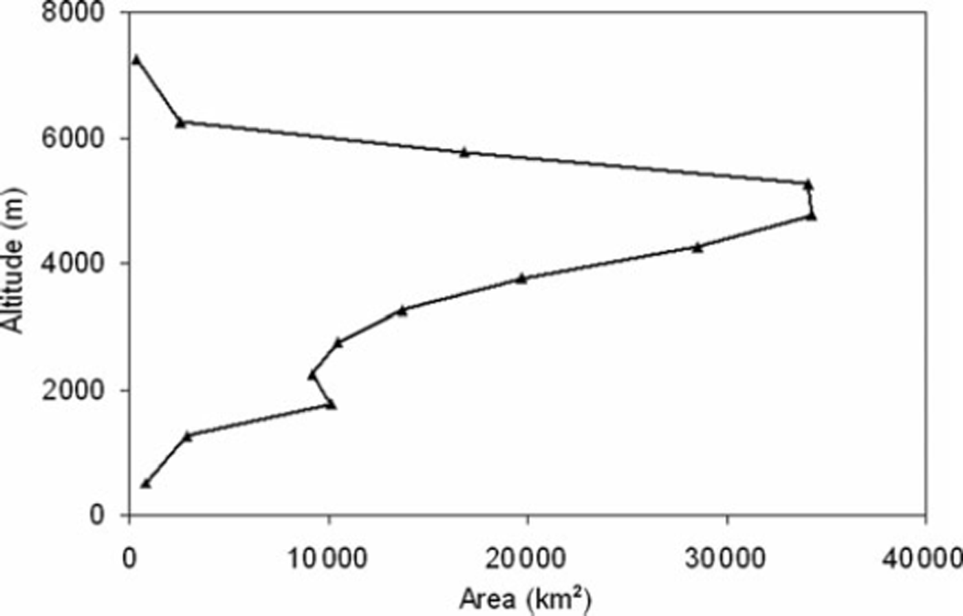
Fig. 4. Area–altitude distribution of the 28 sub-basins in the western Himalaya.
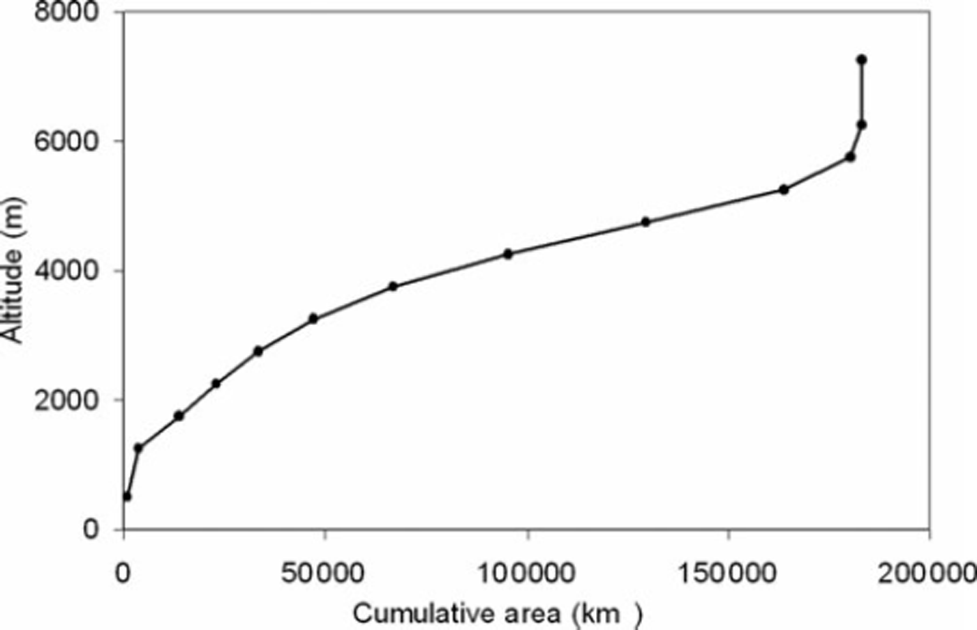
Fig. 5. Hypsographic curve giving total area below each altitude for the 28 sub-basins in the western Himalaya.
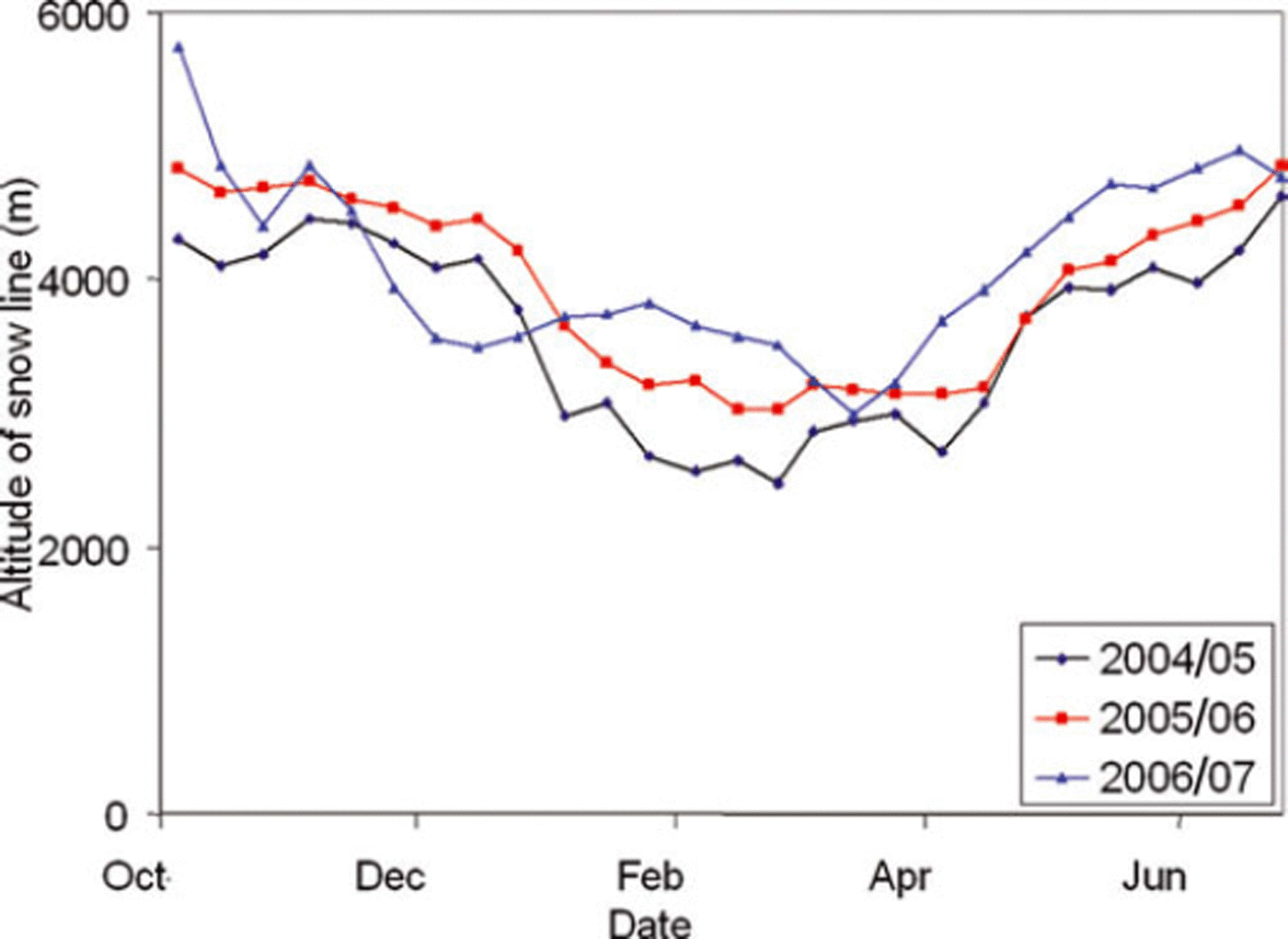
Fig. 6. Overall changes in snow-line altitude in the 28 sub-basins in the western Himalaya.
Table 3. Mean monthly snow-line altitude
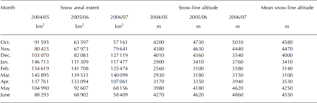
The snow accumulation and ablation curves differ for each basin, depending upon climatologically sensitive zones and altitude distribution of the basin. The Himalayan region is classified into three regions, the lower, middle and upper Himalayan zones, with average snowfall (1990–2004) of 1178, 537 and 511 cm a−1, respectively (Reference Sharma and GanjuSharma and Ganju, 2000; Reference Gusain, Singh, Ganju, Singh, Sarwade and GanjuGusain and others, 2004). For comparative analysis, Ravi and Bhaga basins are selected, located in the south and north of the Pir Panjal range, respectively. The area–altitude distributions of these basins are given in Figure 7. Ravi basin is located in lower-altitude zones. For example, 90% of Ravi is located below 4000 m a.s.l., whereas this value for Bhaga basin is only 20% (Fig. 7). Altitudes of Ravi and Bhaga basins range from 630 to 5860 m, and from 2860 to 6352 m, respectively.
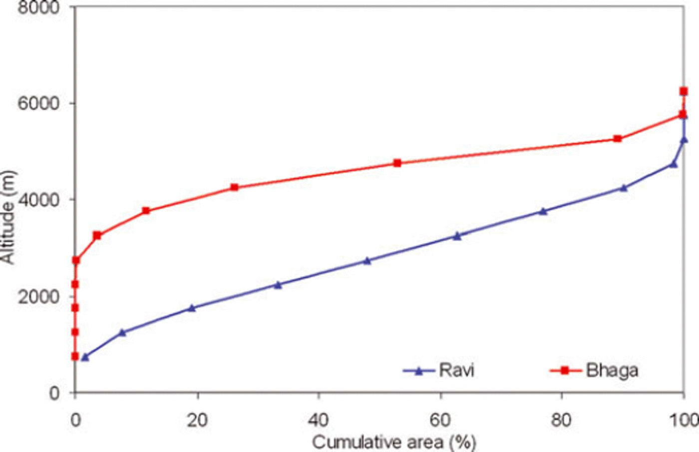
Fig. 7. Hypsographic curves for Ravi and Bhaga river basins.
In Ravi basin, snow accumulation and ablation are continuous processes throughout the winter. Even in midwinter, melting of a large snow area was observed: in January 2005, snow area was observed to be reduced from 90% to 55%; similar trends were observed for 2005/06 and 2007/08 (Fig. 8). In summer, snow ablation was fast: almost 50% of the snow cover melted within a period of 1 month, and by the end of June almost 80% of the snow cover had melted.
In Bhaga basin, snowmelting was observed in the early part of the winter, i.e. in December. Snowpack was stable from mid-January to the end of April (Fig. 9). This observation is consistent with earlier observations made in Baspa basin (Reference Kulkarni and RathoreKulkarni and Rathore, 2003). Baspa is a high-altitude basin located on the northern side of the Pir Panjal range. In this basin, significant snowmelt was observed in December, influencing stream runoff. These observations suggest that river basins respond to climate change depending on geographical location and altitude distribution.
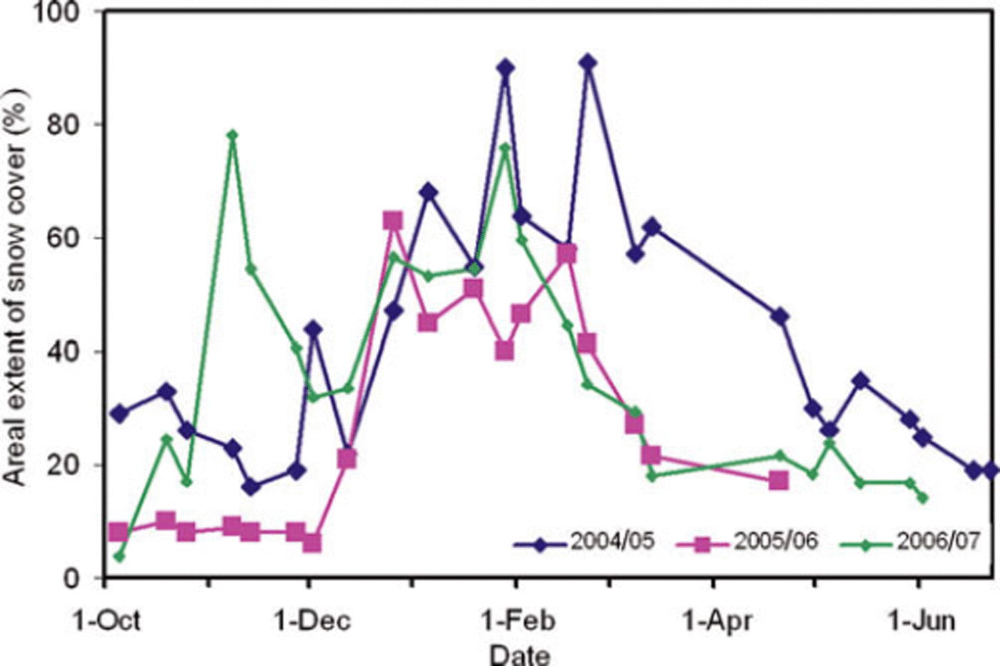
Fig. 8. Snow-cover depletion curve for Ravi river basin for 2004/05, 2005/06 and 2006/07.
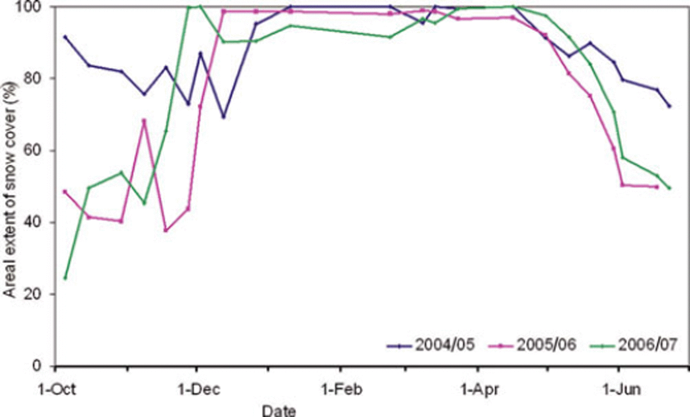
Fig. 9. Snow-cover depletion curve for Bhaga river basin for 2004/05, 2005/06 and 2006/07.
6. Conclusions
This paper describes the analysis of the snow-cover variability of 28 sub-basins in the central and western Himalaya. Approximately 1500 AWiFS scenes were processed and analyzed to generate (5 d)−1 and (10 d)−1 snow-cover maps using an NDSI-based algorithm for three years (2004/05, 2005/06 and 2006/07) from October to June. Area–altitude distribution of snow-cover variability was studied using SRTM data over the Himalayan range for all 28 sub-basins. An analysis of low-altitude basins like Ravi basin and high-altitude basins like Bhaga basin showed a different trend of snowmelt in summer and winter months. A significant amount of snowmelt was observed throughout the winter for basins such as Ravi, and at the beginning of winter for basins such as Bhaga and Baspa. This has potential to influence the stream runoff pattern of numerous Himalayan streams.
Acknowledgements
This investigation was carried out under Snow and Glacier Studies Project, a joint initiative of the Indian Ministry of Environment and Forest (MoEF) and Department of Space (DOS). We are grateful to. R.R. Navalgund for continuous guidance and encouragement during the investigation. We thank T.J. Majumdar for suggestions and comments on the manuscript.


