


Introduction
Numerous studies demonstrate that the strong emissivity differences between ocean, ice and land can be exploited to investigate the seasonal evolution of polar snow and ice. Most passive microwave research has concentrated on variation in annual sea-ice advance and retreat along with more recent attention on terrestrial snow cover. Analysis of passive microwave data over polar ice sheets has been the subject of several papers (Reference Zwally, Comiso, Parkinson, Campbell, Carsey and GloersenZwally and others, 1983; Reference Parkinson, Comiso, Zwally, Cavalieri, Gloersen and CampbellParkinson and others, 1987). Typically, passive microwave analysis involves merging several channels to refine an estimate of a specific geophysical variable (e.g. sea-ice concentration). In this paper we rely on a single channel of data draped over a digital elevation model of Antarctica. By time-sequencing passive microwave images, portrayed on this three dimensional representation, we can develop new intuition about the interaction between the southern ocean, atmosphere and ice sheet.
Analysis
The DEM data were provided by the National Snow and Ice Data Center in the form of a raster file. The DEM is described in a letter report by Ian Smith dated 1985 provided with the data. Essentially it consists of a 281 × 281 celled record of surface elevations derived from the SPRI Glaciological and Geophysical folio (Reference DrewryDrewry, 1983). Futher information about how the elevations were assigned to the 281 × 281 grid can be found in a report by Reference Radok, Brown, Jenssen, Smith and BuddRadok and others (1986). This report states that a 20 km grid was projected onto the SPRI Folio map and elevations were interpolated onto the grid intersections.
Original elevation data come from a variety of sources; each contains errors related to the region, terrain roughness, weather conditions and measurement devices. On average the elevation data are considered accurate to a few tens of meters.
Data are presented on a polar stereographic projection with a standard latitude of 71°S. The X,Y origin is centered at the South Pole. The grid spacing is quoted as 20 km (on the projected surface). Elevations are assigned to the grid-line intersections which can be assigned either I, J positive, integer array labels or corresponding Χ, Y values in kilometers. X and Y values are only approximations of distance in kilometers, derived from the map’s scale. This projection is not equal distance and therefore the map scale is distorted to some extent except along the standard parallel.
The projection formulas used to assign elevations to each DEM data point are provided in Smith’s report, which documents the DEM file and can be used to transform the X, Y data to latitude, longitude. Once the elevation-point locations are assigned to latitudes and longitudes the data are projected onto the SSM/I plane, which is a polar stereographic plane with a standard latitude of 70°S. The projection formulas used to convert the latitudes and longitudes to Χ, Y values are given in the SSM/I users’ guide, provided with the SSM/I information distributed on CD-ROM (NSIDC, 1990). Using these equations, the DEM elevations were projected onto the exact plane which the SSM/I data reside. Because the original DEM and SSM/I projection planes and grid spacings do not match, the elevations are not immediately coincident with the SSM/I values. The diagram in Figure 1 illustrates the orientation of DEM data with respect to the SSM/I data. Not only did the original data assignment locations differ between the two data sets, the DEM locations projected onto the SSM/I plane were no longer at their original 20 km intervals. This can be explained by the fact that a set of longitudes and latitudes which constitute an equal interval square grid on one projection, generally will not represent a square grid given new projection parameters. Conse¬quently, the re-projected DEM is no longer a regularly spaced grid.
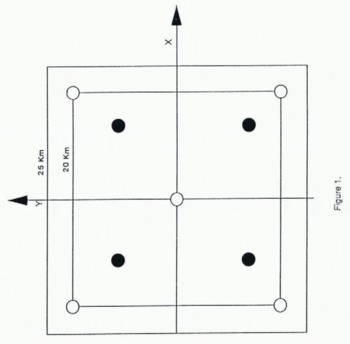
Fig. 1. Sketch of 25km SSM/I grid with data value assignment locations marked by black circles. The SSM/I Tb assignment locations are in the center of each 25 km grid cell. They begin at 12.5 km and are spaced at 25 km intervals. The DEM grid is overlaid and the elevation assignment locations are marked by the hollow circles. They are assigned to the intersections of a 20 km grid, starting from the origin and spaced at 20 km intervals.
There is a displacement between the original and projected data-point locations relative to the origin because the standard latitude used to project the original DEM is different from that used for the SSM/I grid. The displacement is approximately 88 km for the outermost grid cell; the displacement is less than 25 km at the ice-sheet margin. Calculations show that this displacement is more than expected, probably because different earth models were used to create each grid. As we can see, this type of projection is neither suited nor intended for preservation of distances. It is chiefly used for navigation because of its preservation of angles. Although the elevation data-point locations are altered by the transformation, they are not less reliable. The elevation data can now be expected to share the same planer distortions as the SSM/I data and thus are co-registered.
Elevation data were resampled to pair elevation and brightness temperature data. Many methods are avail-able for this recursive problem, such as the closest neighbor, maximum, average or minimum neighbor methods; and many interpolation methods (Reference ClarkClark, 1990, p. 45–47, 204–237). The area over which information is integrated is called here the “area of effect”. The choice of this area (neighborhood), or radius from the data assignment locations on the SSM/I grid, can significantly affect the end result.
An interpolation routine was used to estimate the elevations at the required locations. Interpolation with appropriate weighting functions tends to preserve trends in the data set. We adopted a distance-weighted interpolation method using the Shepard algorithm (Reference Lancaster and SalkauskasLancaster and others, 1986, p. 62–64). The algorithm interpolates by using weighted distance values from the Tb data-point location to existing elevation points which fall within the specified radius. Because an interpolated point will at times fall nearly on an existing elevation point, we prefer to use the existing value by setting the smoothing parameter of the algorithm to be zero. The radius of effect for the interpolation routine was chosen to include only immediate neighbors. Due to the grid spacing of the original DEM, the farthest distance an immediate neighbor could be is approximately 20 km. One concern was that interpolated elevation points could be distorted by any large neighboring change and so it was not possible to ensure that a rapid change in slope, such as a mountain peak, would not be significantly smoothed by the interpolation. Because this research focuses on the ice sheet, distortions in mountainous regions were ignored.
Once the DEM data have been interpolated onto the SSM/I grid, they are converted from the new Χ,Υ,Ζ coordinates into the format of the SSM/I data. This can easily be accomplished by first converting the X and Y values to I and J cell values, again using conversion formulas supplied in the SSM/I documentation, and placing the elevation values into corresponding array cells.
Error Analysis of the New Dem
We considered the DEM as a database without errors. Moreover we assume that there were no unaccountable distortions introduced in creating the DEM that was co-registered to the SSM/I map projection. We were concerned that interpolating the co-registered DEM data points to the exact node location of SSM/I data might introduce unacceptable errors because of the facts that first we were interpolating from an irregularly spaced to a regularly spaced grid and second that the grid spacing increased from 20 to 25 km resolution. A blunder check for the interpolation procedure was made by comparing the very limited number of discrete locations where the co-registered and the final, interpolated grids matched exactly. The statistical results from comparing these few nodes suggests that the original elevation values were preserved to within about 1 m.
To increase the number of nodes available to test the integrity of the interpolated data set, we re-interpolated the final 25 km DEM grid back down to about a 20 km test grid that closely approximated the irregular grid. We compared data points on the test DEM to data from the DEM co-registered to the SSM/I projection. Again, the co-registered DEM had an irregular grid spacing so it was not possible to match elevation points exactly to the test DEM. Therefore we compared points on the two DEMs only where the range difference between the data ponts was less than a predefined tolerance. A total of 7276 pairs of elevation points selected from across the entire continent were found to fall within our tolerance limit. The average difference in elevation was found to be about 12 m with a standard deviation of 45 m. This suggests that there was no substantial bias or trend introduced into the elevation data by the interpolation scheme. Comparison of the test and co-registered DEMs revealed an elevation anomaly of 783 m at X = 118.9 km and Y = −673.8 km, a location in the Transantarctic Mountains. We attribute this anomaly to two processes. First the Χ, Y coordinates of the point in the test DEM were not identical to the coordinates of the point in the co-registered DEM because the later data were irregularly spaced. To compare elevations at a more nearly co-located position, we linearly interpolated the elevation from the nearest neighbors on the test grid to the equivalent location on the co-registered grid. The elevations at these points differed by 185 m. This difference is not surprising given the surface relief in this region and accordingly we place less confidence in the integrity of the final DEM over this type of terrain.
We next compared the test and co-registered DEMs over East Antarctica. This is an area of gently sloping terrain and is more directly the focus of our ice-sheet research objectives. Using a total of 1756 data pairs, we found that the DEM elevations matched to within about 3 m. These differences are insignificant for our purposes.
Discussion
We have so far co-registered the DEM with 37 GHz, vertically polarized brightness temperatures acquired by the Special Sensor Microwave imager for the period beginning December 1988 and ending December 1989. The image projection parameters selected for our present analysis highlight the Pacific sector of Antarctica. An example of mid-summer and mid-winter imagery is shown in Figure 2. The vertical exaggeration is approximately 300 times the elevation. The deep blue color (200 K) around the perimeter of each image represents open ocean. Spiralling storm systems that rotate about the continent are revealed as gray filaments (215 K). Sea ice is indicated by the warm red (250 K) and yellow (265 K) patterns encircling the continent in winter; sea ice is largely absent in the summer scene. Sea-ice brightness temperatures are strongly influenced by the presence of storms and it is possible to visually track storm systems that sweep across the sea-ice cover by observing similar trends (but not magnitudes) of brightness temperature. When several scenes are sequenced, it is also possible to observe storm systems that develop in the Amundsen Sea and gather sufficient energy to ride up and over the Ford and Rockefeller mountains, eventually draining off into Marie Byrd Land and the Siple Coast (irregular yellow pattern in left central part of the condensed images in Figure 3). Finally, the small, relatively warm object identified on each image of Figure 2, is the iceberg B-9, which can be tracked from its point of origin to its collision with the north Victoria Land coast.
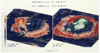
Fig. 2. SSM/I Tb data draped over the DEM. The orientation of the view highlights the Ross Ice Shelf area. The elevations are exaggerated to 300 times normal, for visualization purposes. The left image demonstrates Tb signatures during the austral mid-summer and the right image is during mid-winter. The color bar can be used to associate selected Tb values with an assigned color. The iceberg B-9 is highlighted by the circles.

Fig. 3. SSM/I Tb data draped over the DEM. The eight images represent Tb values over eight consecutive days in December 1988. These images show the evolution of a storm system in the Amundsen Sea and the translation of that storm over the Ford and Rockefeller mountains into Marie Byrd Land. The storm appears as a yellow band which progresses from the Amundsen Sea towards the Ross Ice Shelf.
Seasonal variations in brightness temperatures over the interior ice sheet are driven largely by the annual physical temperature cycle (Jezek and others, 1990). Brightness temperature patterns over East Antarctica correlate roughly with elevation (Fig. 2). This is to be expected because of the well-known relationship between physical temperature and elevation over much of Antarctica. Cold brightness temperature anomalies, at least as compared to the elevation contours, do appear over the interior of Wilkes Land. Here, elongated brightness temperature patterns (about 18 Κ in the summer scene of Figure 2) appear uncorrelated with other geophysical variables such as wind direction or strength.
There is almost no correlation between brightness temperature and elevation in West Antarctica. For example, there is a strong brightness contrast (almost 30 K) between the Ross Sea and Amundsen/Bellingshausen Sea drainage basins that parallels very closely the topogrpahic ridge that defines these drainage basins. Presumably, the warm, moist air masses that contribute to the high acumulation rates observed on the Amundsen Sea side of West Antarctica are depleted of both moisture and heat when they finally reach the region of the West Antarctic ice streams. Consequently, this later area appears in this microwave channel more similar to the deep interior of East Antarctica. It is also interesting to note that in this same area, Siple Dome appears as a warm brightness temperature anomaly throughout the year.
We have sequenced 13 months on microwave brightness temperature data draped on the DEM for display as an animation, recorded on video-tape. As alluded to above, the inclusion of time as part of the data-inspection process adds considerably to the investigators’ intuition about the processes occurring on the ice sheet and surrounding ice-covered water. For example, the animation provides insight into the effect of weather on brightness temperatures over sea ice. By noting the translation of storm systems from open ocean onto sea ice, it may be possible to validate sea-ice-concentration weather-correction algorithms by checking whether the brightness temperature pattern associated with the storm is preserved or eliminated in the ice concentration product by the application of a particular algorithm. The animation also helps delimit certain areas and times for more focused study. Assessing the frequency and intensity of West Antarctica storm systems as revealed in the passive microwave data is a good example. Finally, the animation coupled with the DEM overlay can highlight new and unexpected phenomena. The relation¬ship between katabatic wind fields and warm temperat¬ure anomalies on AVHRR thermal imagery is well-established (Reference BromwichBromwich, 1989). There also seems to be a relation between katabatic drainage patterns and the passive microwave data (Fig. 2). In this case the drainage patterns are associated with relatively cold brightness temperature anomalies that are persistent throughout the year. This observation suggests that the wind fields are modifying the physical properties of the ice-sheet surface.
Consequently, the passive microwave data are more an indicator of the seasonal patterns of flow rather than an indicator of individual, transient events.
Acknowledgements
This research was supported by the Polar Oceans Program of NASA Headquarters. Appreciation for technical support is extended to Eduardo Falcon, and Rob Schmedly (Center for Mapping, The Ohio State University), and to Steve Grace (Ford Motor Co.).


