Introduction
Understanding variability of Sea ice in polar regions is of crucial importance to clarify the mechanism of climate change on a global Scale. Satellite remote Sensing has revealed the long-term variability of Sea-ice extent (e.g. Reference Zwally, Comiso, Parkinson, Cavalieri and GloersenZwally and others, 2002). however, deriving Sea-ice thickness by Satellite remote Sensing requires further development. thus, in terms of Sea-ice thickness, field observations on a large geophysical Scale are very important. in the arctic, extensive observations have been conducted and the accumulated data Show Some evidence of a decline in the mean ice thickness. however, in the antarctic, our knowledge of Sea-ice thickness distribution is much less extensive (Reference WadhamsWadhams, 2000). accumulation of field data is Strongly required in the antarctic for verifying how Sea ice in the antarctic responds to climate change.
The japanese antarctic research expedition (jare) has conducted Ship-based observations of Sea-ice thickness and Snow depth on board the antarctic research vessel, icebreaker shirase. during the december 1987–february 1988 voyage, one of the authors initiated Sea-ice thickness and Snow-depth observations using a downward-looking video camera (hereafter denoted as video method). video observations were conducted on the next three voyages from december 1988 to february 1991 as a part of the antarctic climate research project by jare (Reference shimodaShimoda and others, 1997). in total, video observations were conducted on 11 voyages between december 1987 and february 2005. additionally, jare has undertaken Sea-ice thickness observations using electromagnetic–inductive (em) instruments Since the december 2000–february 2001 voyage (Reference Uto, Shimoda, Izumiyama, Squire and LanghorneUto and others, 2002).
These observations have been conducted in landfast ice and pack ice. shirase must break the extended landfast ice in lützow-holm bay to access Syowa Station (69.01˚ S, 39.59˚ e). it traverses the landfast ice along a mostly routine passage at about the Same time each year: mid-december to early january for the outbound (to Syowa) voyage, and mid-february for the homebound (from Syowa) voyage. these observations provide a unique and relatively long-term dataset of Sea-ice thickness and Snow depth of the landfast ice. there were relatively few opportunities for observations during homebound voyages, So we analyze only the data for the landfast ice during outbound voyages. we also use Satellite images, which are archived at japan’s national institute of polar research (nipr), to Show the characteristics of Summer landfast ice in lützow-holm bay and its interannual variability.
Measurements
figure 1 Shows the Sea-ice monitoring System which has been on board shirase Since december 2000. em instruments and a downward-looking video camera are installed on the weather deck of the Starboard Side. another video camera is installed at the top of the mast for monitoring Sea-ice concentration (Reference shimodaShimoda and others, 1997).
Fig. 1. Sea-ice monitoring System on board shirase.
Em method
Ship-based em observation of Sea-ice thickness was initiated by Reference HaasHaas (1998) in the bellingshausen and amundsen Seas, antarctica. Since then, em observations have been conducted on board many icebreakers (e.g. Reference Reid, Worby, Vrbancich and MunroReid and others, 2003). a portable, Single-frequency em Sensor (EM31/Ice, geonics ltd) is used to measure the distance from the Sensor to the bottom of Sea ice, Z E (surface of Sea water). a laser distance Sensor (ld90-3100hs, riegl) detects the distance from the Sensor to the Surface of Snow or ice in case of no Snow cover, Z L. Subtracting Z L from Z E gives ice + Snow thickness, Z I (denoted as total thickness). details of em observations are described in Reference HaasHaas (1998).
Video method
One of the most convenient methods for observing Sea-ice thickness and Snow depth is to view the cross-section of broken ice pieces. in the present Study, a downward-looking video camera was installed on the weather deck for monitoring Sea-ice thickness and Snow depth. lützow-holm bay is known as a region with heavy Snow cover. it is reported that the contribution of Snow to the growth of ice is Significant through the formation of Snow ice and Superimposed ice (Reference Kawamura, Ohshima, Takizawa and UshioKawamura and others, 1997). the video method provides unique data of Snow depth. details of video observations are described in Reference shimodaShimoda and others (1997).
Results and Discussions
summary of observations
table 1 is a Summary of the observations conducted in the landfast ice during the outbound voyages of shirase. em observations have been conducted Since december 2000. due to Signal contamination, em data from the december 2001 and 2004 voyages are not available. video observations of the landfast ice were conducted during ten voyages between december 1988 and 2004. although they were conducted in december 1989, few data on the landfast ice are available. no video observations were made between december 1991 and 1996 or in 1998. Snow-depth data are available for eight voyages because Snow depth was not analyzed for the december 1988 and december 1990–january 1991 voyages.
Table 1. Summary of the Ship-based observations of landfast ice during the outbound voyages of shirase
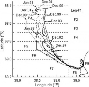
figure 2 Shows ten tracks of shirase in the landfast ice during its outbound voyage. each line begins at the edge of landfast ice, Showing Significant variability in the extent of the Summer landfast ice. figure 3 Shows that the edge varies between 68.4˚ S and 68.9˚ S. the difference is up to about 50 km. in the following analysis, a whole track is divided into nine legs (f1–f9). each leg is about 10km long.

Fig. 2. Tracks of shirase in the landfast ice during outbound voyages. The tracks are divided into nine legs.

Fig. 3. Interannual variability of the northern edge of landfast Sea ice as measured during shirase’s outbound transects from January 1988 to December 2004.
Accuracy of total thickness observations
figure 4 Shows the total thickness comparison between em and drillhole observations. drillhole observations were conducted on the multi-year landfast ice at ongul Strait in leg f9 and off bentenjima island in leg f7 in january and february 2001, respectively. figure 4a Shows that em and drillhole observations at ongul Strait agree reasonably well. figure 4b Shows that both observations off bentennjima island agree reasonably well except for the Section between 50 and 65 m. a relatively large difference in this Section may be due to the influence of an ice block which was broken by shirase and pushed aside under intact ice within the footprint area (∽9m) of the em observations (Reference Uto, Shimoda, Izumiyama, Squire and LanghorneUto and others, 2002).
Fig. 4. Total thickness comparison between EM and drillhole measurements along two transects (top: near Syowa, leg F9; bottom: off Bentenima Island, leg F7).
The average em and drillhole thickness of the two locations were 2.86 and 2.79 m, respectively. the Slight overestimation of total thickness by the em method might be due to the the influence of a broken ice block as described above. the rms difference of em observations against drillhole observations is 0.37 m, which corresponds to about 13% of the average total thickness. we conclude that the em observations are reasonably accurate for thick multi-year landfast ice.
figure 5 Shows the total thickness comparison between the em and video methods. here the averaged total thickness in each leg is plotted. the two methods agree very well for ice about 0.8m thick, but the video method generally gives a Smaller total thickness than the em, and this difference increases as total thickness increases. there are Several possible reasons for this difference. video observations require that ice pieces are turned to an almost upright position. during turning, it was Sometimes observed that Snow cover fell off the ice, and it is probable that Such Samples are included in the total thickness distribution determined by the video method. as described later, Snow depth increases as ice thickness increases, which would result in an increased difference at greater thickness.
Fig. 5. Total thickness comparison between EM and video method. The average value in each leg is plotted as a circle. Solid line indicates a least-squares approximation polynomial.
Although it is easy for relatively thin ice to be turned, thicker ice resists turning. in cases when the ice has high Spatial variability in thickness, it is most likely that only the thinner part of the ice is observed by the video method. furthermore, it was observed that for thick multi-year ice the undermost layer often fell off during turning. the em method Slightly overestimates the total thickness of thick multi-year ice, but provides better total thickness estimates than the video method, particularly for thick ice. the total thickness measured by the video method was corrected using the following least-squares parameterization:
Total thickness distribution observed by EM method
figure 6 Shows the total thickness distribution in december 2000, 2002 and 2003 measured by the em method. although data are measured at a Sampling frequency of 1 hz, values Shown in figure 6 are 10 S time averages. profiles for 2002 and 2003 also contain a Section of pack ice and polynya. in most years, a polynya exists between the landfast ice and the pack ice in Summer. during the outbound voyage in 2000, the ice was So thick that shirase had to back and ram very frequently to break the ice. due to the contamination by a broken ice block under the intact ice (Reference Uto, Shimoda, Izumiyama, Squire and LanghorneUto and others, 2002), Some em data are not available in figure 6a.
Fig. 6. Total ice thickness as measured along outbound voyages using the EM method. Profiles during outbound voyages of shirase in December 2000 (a), 2002 (b) and 2003 (c) are plotted.
The features of the total thickness distribution of the Summer landfast ice are described with reference to the december 2002 profile (fig. 6b). from leg f5 to f7, the total thickness is rather constant at about 1.5 m. near the boundary between legs f7 and f8, there is discontinuity in the total thickness profile, i.e. an increase from about 1.5 to 4 m thick. this reflects the past break-up of a part of landfast ice (Reference UtoUto and others, 2004). figure 7e and l Show us national oceanic and atmospheric administration (noaa) advanced very high resolution radiometer (avhrr) images of lützow-holm bay in may and december 2002, respectively. figure 7e Shows a break-up at almost a maximum extent, while figure 7l is taken at almost the Same time as the Ship observations. a large extent of landfast ice was lost due to break-up 7 months before the Ship observations. part of this refroze as first-year ice between legs f5 and f7 in december 2002. the intersection between the track of shirase and the break-up boundary in may 2002 corresponds to the discontinuity in the total thickness profile. multi-year ice was present in legs f8 and f9.

Fig. 7. Noaa Avhrr ch1 or ch4 images of winter (top) and Summer (bottom) landfast ice in Lützow-Holm Bay. Dates are dd/mm/yy. By courtesy of National Institute of Polar Research, Japan.
figure 6b Shows that the total thickness of multi-year ice in legs f8 and f9 decreased gradually toward the antarctic continent. this is due to the influence of Snow cover on the development of Sea ice in the coastal area. Reference Fedotov, Cherepanov, Tyshko and JeffriesFedotov and others (1998) reported that Snow depth on the landfast ice decreases in the nearshore zone, due to Scouring by continental winds of constant direction. Reference Kawamura, Ohshima, Ushio and KakizawaKawamura and others (1993) conducted a 2 year Study on the growth of Sea ice and Snow cover in ongul Strait (in leg f9) in 1990 and 1991. they reported that the Snow depth and ice thickness decreased toward the Shore throughout the year. Reference Kawamura, Ohshima, Takizawa and UshioKawamura and others (1997) also reported that the Snow depth increased consistently with distance from the Shore, and the Spatial variation of Sea-ice thickness was correlated well with the Snow depth. in general, the Snow cover acts as an insulator and prevents ice from melting in Summer. in an area of heavy Snow like lützow-holm bay, it also enables upward growth in Summer by Snow-ice and/or Superimposed-ice formation (Reference Kawamura, Ohshima, Takizawa and UshioKawamura and others, 1997). less Snow thus leads to thinner multi-year ice in legs f8 and f9.
Reference Fedotov, Cherepanov, Tyshko and JeffriesFedotov and others (1998) reported that the maximum Snow accumulation on east antarctic landfast ice occurred at a distance of 6–15 km from the Shore. Reference Kawamura, Ohshima, Takizawa and UshioKawamura and others (1997) reported that the Snow depth reaches a nearly constant maximum value during the austral winter at distances greater than 30 km from the Shore in lützow-holm bay. f. nishio (personal communication, 2004) conducted an extensive Survey of the Snow depth in december 2001–february 2002 and found that it peaked at about 30 km west of Syowa Station. figure 6a Shows that the total thickness Starts to decrease in the middle of leg f7, about 20 km from the Shore. thus 20–30km is a typical distance for drift-snow accumulation in lützow-holm bay, which is Somewhat greater than the distance cited by Reference Fedotov, Cherepanov, Tyshko and JeffriesFedotov and others (1998). f. nishio (personal communication, 2004) also found that the Snow drifted to the Southwest, and, Since the area around Syowa Station has a relatively weak katabatic wind, frequent blizzards with a Strong northeasterly wind (e.g. Reference schwerdtfeger and OrvigSchwerdtfeger, 1970) are probably responsible for Snow transport near the Shore.
Interannual variability of total thickness and Snow-depth distribution
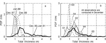
figure 8 Shows the probability density function (pdf) of total thickness for ten voyages. here the total thickness from the video method is corrected using equation (1). from figure 8, the pdfs can be categorized into three types. type a has a broad modal thickness of about 1.5 m and a relatively long tail. pdfs for december 1990–january 1991 and december 2000 correspond to this type. type b has a Sharp peak at a modal thickness ranging from 0.8 to 1.4 m. pdfs for january 1988, december 1988, 2003 and 2004 fall into this category. type c is intermediate between types a and b. december 1997, 1999, 2001 and 2002 belong to this type.

Fig. 8. Pdf of total thickness estimated from the video method. (a) Four voyages from January 1988 to December 1997. (b) Six consecutive voyages from December 1999 to December 2004. Total thickness data are corrected by equation (1). Thick Solid lines indicate type A, the thickest type of PDF. Dashed lines indicate type B, the thinnest type. Thin Solid lines indicate type C, an intermediate between types A and B.
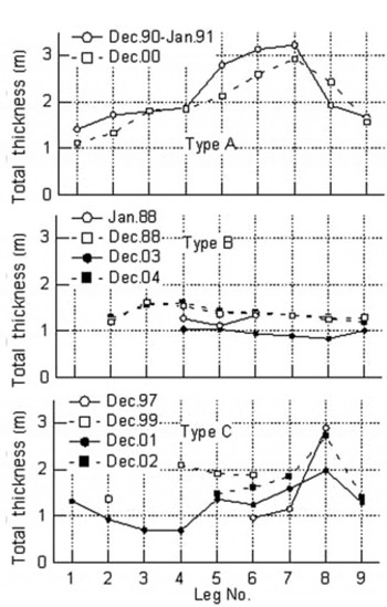
Leg-averaged total thickness and Snow depth are plotted against leg number in figures 9 and 10, respectively. again, the total thickness from the video method has been corrected using equation (1). Snow thickness data from video observations are available for eight voyages (table 1). figure 9 Shows that each type of pdf has a different profile of leg-averaged total thickness. for type a (two profiles) the total thickness increases monotonically toward the South and reaches a maximum of up to 3m in leg f7. it then decreases toward the Shore. in contrast, type b (four profiles) has a flat distribution and no peak around leg f7. in the profiles of type c, total thickness has a peak of 2–3m in leg f8, with a Significant decrease in total thickness between legs f8 and f9.

Fig. 9. Profiles of leg-averaged total thickness distribution by video method. Eight profiles are categorized into (a) type A, (b) type B and (c) type C. Total thickness data are corrected by equation (1).
Fig. 10. Leg-averaged Snow-depth distribution by video method.
The Snow-depth profiles (fig. 10) are very Similar to the total thickness profiles (fig. 9). figure 11 Shows the relation between leg-averaged Snow depth and the total thickness for eight voyages. linear regression gives the following:
Fig. 11. Relation between total thickness and Snow depth. Both Snow and total thickness data are leg-averaged, and total thickness data are corrected using equation (1). The Solid line is a regression fit, giving the Snow depth as 0.168 times the total thickness, or Snow depth as 0.20 times the ice thickness.
Or
Factors influencing the interannual variability of total thickness distribution
Reference UshioUshio (2003) investigated the interannual variability of Sea-ice break-up in lützow-holm bay from 1980 to 2003. he Suggested that a Southeasterly wind field, Shallow Snow depth and mild winter prior to the break-up are factors which favor break-up events. figure 7 Shows that there is Significant interannual variability in the extent of break-up in winter. for example, a relatively large area of landfast ice remained in 2000 (fig. 7c). Reference UtoUto and others (2004) reported that the annual break-up location in 1990 was almost the Same as that in 2000. on the other hand, break-up extended to the Shore in june 2004 (fig. 7g) and no multi-year ice is included in the total thickness profile for december 2004. figure 7f Shows that a very Small area of landfast ice remained in winter 2003. in 1997, 1999, 2001 and 2002, the area of landfast ice in winter was between those in 2000 and 2003.
As described before, 20–30km is a typical distance for drift-snow accumulation. if the extent of break-up in winter is Small and does not reach this distance, there is much ice with abundant Snow cover that can develop into thick multi-year ice. this gives the type a pdf in 1990 and 2000. if the extent of break-up is large and reaches this distance, less ice is available to develop into thick multi-year ice, and a type c pdf results. if the break-out encroaches even closer to the Shore, the extent of thick multi-year ice diminishes and results in a type b pdf. in Summary, interannual variability in the total thickness of multi-year ice primarily reflects the extent of the break-up of the landfast ice and its interaction with drift Snow in the nearshore zone.
The Second factor influencing the interannual variability of the total thickness distribution is the duration of first-year ice development. Reference UshioUshio (2003) reported that typically a Series of Successive break-up events Starts in march and ends in july or august. thus december first-year ice has grown for 4–5 months and is typically up to 1.5m thick. however, figure 9 Shows that the leg-averaged total thickness of first-year ice has Significant interannual variability, ranging from 0.7 to 1.8 m. in 1997, the break-up events Started in july 1997 and did not finish until july 1998 (Reference UshioUshio, 2003). a Similar phenomenon was observed in 2003. the consequent Short growth times resulted in relatively thin first-year ice in december 1997 and 2003.
The good correlation between ice thickness and Snow depth in figure 11 Suggests that Snow depth influences the interannual variability of total thickness distribution. however, it Should be noted that the influence of break-up is also included in the relation between Snow depth and total thickness in figure 11. as Shown in figure 7c–f, winter Sea ice in leg f9 endured from december 2000 to 2003. in order to investigate the influence of Snow depth on the interannual variability of ice thickness, the temporal distributions of total thickness and Snow depth at leg f9 for this period are plotted in figure 12. unfortunately, there are no data available on the Snow depth at leg f9 in december 2000. a gradual decrease of total thickness occurred from 2000 to 2003. on the other hand, a Slight increase of Snow depth is observed from 2001 to 2003.
Fig. 12. Interannual variability of total thickness and Snow depth in leg F9. Total thickness data are corrected by equation (1).
Reference Wu, Budd, Lytle and MassomWu and others (1999) discussed the effect of Snow depth on the accretion and ablation of antarctic Sea ice using a coupled atmosphere–sea-ice model. they reported that, over most of the antarctic Sea-ice zone, winter ice was thicker both when there was no Snow cover and when the Snow cover was twice that in their Standard model. Reference Powell, Markus and StösselPowell and others (2005) obtained Similar results. these results indicate that Sea-ice thickness has a negative correlation against Snow depth if the amount of Snow is Small, as in leg f9. further data are needed to clarify the influence of Snow depth on the interannual variability of total thickness distribution.
Conclusions
We investigated the characteristics of Summer landfast ice in lützow-holm bay, using data on the total thickness distributions from Ship-based em observations, total thickness and Snow-depth distributions from Ship-based video observations and noaa avhrr Satellite images. there is Significant interannual variability of the total thickness of Summer landfast ice in lützow-holm bay. this primarily reflects the pattern of break-up of the landfast ice Since the extent of break-up determines the fraction of first-year ice and multi-year ice. Strong northeasterly wind causes Snowdrift and redistribution within a distance of 20–30km from the Shore, and in this region Snow depth and ice thickness gradually decrease toward the Shore. this is because thinner Snow cover enhances melting of ice and is not conducive to the growth of Superimposed ice or Snow ice in Summer. interannual variability of the total thickness of multi-year ice primarily reflects the interaction between the extent of the break-up of the landfast ice and the Snowdrift in the nearshore zone. the duration of Successive break-up events determines the length of the growth Season, and hence the thickness of first-year ice.
Acknowledgements
We express Sincere gratitude to f. nishio and h. wakabayashi (jare43), g. hashida (jare44), k. azuma (jare45) and a. furusaki (jare46) for conducting Ship-based observations.we thank the captains and crews of icebreaker shirase for their cooperation, and a. enokihara for analyzing the video thickness data. noaa avhrr images were received at Syowa Station and archived in the computing and communications center of nipr. we thank n. hirasawa of nipr for assistance in using noaa avhrr images.