


Introduction
When polar ice is formed by dry sintering, bubbles of atmospheric air are enclosed in it. Air extracted from ice samples representing the late part of the last glaciation shows a considerably lower CO2concentration than does air extracted from ice representing the Holocene period (Reference Berner, Oeschger and StaufferBerner and others 1980, Reference Delmas, Ascencio and LegrandDelmas and others 1980, Reference Neftel, Oeschger, Schwander, Stauffer and ZumbrunnNeftel and others 1982). There is little doubt that this change in CO2 concentration is due to a change in the atmospheric CO2 concentration. Due to experimental difficulties, poor ice-core quality or uncertainties in the dating of ice samples it was not possible until recently to investigate the history of the increase of the atmospheric CO2 concentration with a sufficient time resolution. The availability of the ice core drilled at Dye 3 (south Greenland) during the Greenland ice Sheet Program, and improvements in analytical techniques (Reference Neftel, Oeschger, Schwander, Stauffer and ZumbrunnZumbrunn and others 1982) have now made such investigations possible.
Measurements on samples from the Dye 3 ice core, covering the transition from the last glaciation to post-glacial times, showed an unexpectedly rapid increase of the atmospheric CO2 concentration (Reference Stauffer, Neftel, Oeschger and SchwanderStauffer and others in press). The mean annual air temperature at Dye 3 is at present −19.6°C and the temperature increases above the freezing point regularly every summer, causing the formation of melt layers. The CO2 concentration in the bubbles of melt layers is increased, because CO2 is very soluble in water, and because the CO2 surplus may not escape completely during refreezing (Reference StaufferStauffer 1981). The temperature at Dye 3 was lower during the transition from the last glaciation to the Holocene than it is at present and the formation of melt layers during this period probably did not occur. One ice sample from the last glaciation showed a significantly elevated CO2 content. Because of this result we wished to investigate whether there were CO2 concentration changes during the last glaciation, and to find out if they were related to climatic changes seen, for example, in the δ18O record. During the ice age the temperature was even lower than during the transition period and we have, therefore, further reasons to exclude the possibility of the formation of melt layers. In the present paper we report results obtained with ice samples representing the period from about 40 to 30 ka BP (Reference DansgaardDansgaard and others 1982: fig.1) which we investigated for changes of the atmospheric CO2 concentration during this period and to see how such changes could be correlated with the δ18O changes. According to Dansgaard this sequence, which shows large, rapid changes in the δ18O values, corresponds to the beginning of Emiliani’s isotope stage 2 (Reference EmilianiEmiliani 1966). It was a period of ice build-up on the continents.

Fig. 1 δ18O profile along the lower part of the ice core from Dye 3 as a function of the distance from bedrock (from Reference DansgaardDansgaard and others 1982, with changes). The line to the right of the profile indicates the core increments discussed in this paper.
Experimental Procedures
For the CO2 analysis ice cubes with each side measuring 1.3 cm are prepared with a band saw. Any part of the cube has a distance of at least 0.5 cm from the original ice-core surface. The ice cubes, each weighing about 2 g, are crushed between two needle matrices in a container which has been evacuated previously to a pressure of about 0.1 Pa. The air in bubbles, which are opened by the crushing, expands over a cold trap (for removing water vapour) into the absorption cell of an infrared laser spectrometer (IRLS). The efficiency of gas extraction by crushing is about 75%, the gas pressure in the absorption cell being about 120 Pa. If the air is enclosed in clathrates the efficiency is a few percent less, but the gas composition shows no measurable changes (Reference Neftel, Oeschger, Schwander and StaufferNeftel and others 1983). For the concentration measurements, during the five minutes after crushing, the laser is tuned several times over an absorption line of the CO2 molecule. After each sample a calibration is performed by passing a standard gas through the crushing device and cold trap and into the absorption cell, at the same pressure as the previous sample. The calibration measurements allow us to determine the stability of the laser system which may change slightly from day to day. Under stable conditions the accuracy of the determination of CO2 concentration in air extracted from 2 g of ice is 2% (6 ppm CO2 concentration). More details concerning the analytical procedure are given by Reference Neftel, Oeschger, Schwander, Stauffer and ZumbrunnZumbrunn and others (1982).
A detailed δ18O profile along the lower part of the Dye 3 ice core has already been measured by Reference DansgaardDansgaard and others (1982). Since we wish to examine in detail a possible correlation between CO2 and δ18O we measured CO2 concentration and δ18O simultaneously on the same ice samples.
Results
From the Dye 3 core, 3 cm thick discs of 25% of the core cross-section were cut every metre from 1 860 to 1 889 m depth below the surface (148 to 177 m from the bottom). From each disc six cubes for CO2 measurements and one sample for δ18O analysis were prepared. The results of the CO2 analyses are shown in Figure 2(a) and the δ18O results in Figure 2(b). The correlation of the CO2 concentration with the δ18O values is obvious, and no phase shift between the two parameters is observable. To investigate the question of a possible phase shift of less than one metre. we measured a set of samples every 0.1 m in the depth interval 1 896 to 1 899 m (138 to 141 m from the bottom). The results of the CO2 measurements are shown in Figure 3(a) and the results of the δ18O measurements in Figure 3(b). In spite of the better resolution no lag between CO2 concentration and δ18O values is observable. This finding is surprising. Even if the climatic events causing the changes of the two parameters were simultaneous we would expect a lag, since the ice and the enclosed air of an ice sample have different ages (Oeschger and others in preparationFootnote *). The age difference at Dye 3 at the present temperature and annual precipitation is about 100 a, which at the depth in question would correspond to about 0.3 m difference in depth. It is not possible to determine the lag to an accuracy better than a few centimetres, but the comparison of Figure 3(a) and (b) suggests that it is less than 0.2 m. This would indicate that the CO2 increase occurred almost simultaneously or eventually lagged the climatic change indicated by δ18O by up to about a century, but this conclusion is tentative.
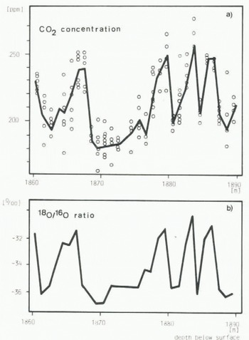
Fig. 2 CO2 and δ18O values measured on ice samples from Dye 3, The 30 m increment corresponds to about 10 ka.
-
(a) Circles indicate the results of single measurements of the CO2 concentration of air extracted from ice samples. The solid line connects the mean values for each depth.
-
(b) The solid line connects the δ18O measurements made on one sample every metre.

Fig. 3 CO2 and δ18O values measured on ice samples from Dye 3. The 3 m increment corresponds to about 1 ka.
-
(a) Circles indicate the results of single measurements of the CO2 concentration of air extracted from ice samples. The solid line connects the mean values calculated for increments of about 0.1 m.
-
(b) The solid line connects the δ18O measurements done on 0.1 m core increments.
Changing Atmospheric CO2 Concentration: Fact or Artefact?
A variation of the atmospheric CO2 concentration is one of several explanations of the CO2 results. In view of the correlation of the CO2 with the δ18O results, there are other possibilities. One is that the concentration of chemical constituents, especially carbonates, changes with the δ18O and that part of the CO2 in the bubbles reacts with these constituents. Based on earlier investigations (Reference Berner, Oeschger and StaufferBerner and others 1980) we reject this hypothesis. Another possibility is the influence of melt layers. According to Reference Stauffer, Neftel, Oeschger and SchwanderStauffer and others (in press) a melt-layer contribution to total ice of about 5% is needed to give an increase of CO2 concentration of 50 ppm. This melt-layer contribution is large; it occurs at Dye 3 under present climatic conditions (Reference Herron, Herron and LangwayHerron and others 1981). Camp Century (north Greenland), with a 4.4°C lower mean annual air temperature, shows narrow melt layers only in extremely warm summers, and the total thickness of melt layers in 50 m of firn is less than 0.15 m (H B Clausen personal communication). The mean annual air temperature at Dye 3 during the glacial period studied is not known, but the highest δ18O value in that core section (−30.2‰) is lower than the present mean δ18O at Camp Century of −29‰ (Reference Dansgaard, Johnsen, Clausen and GundestrupDansgaard and others 1973). It is not possible to correlate δ18O directly with temperature, but the comparison suggests that melt layers did not form at Dye 3 during the period studied. It is in any case very unlikely that there were so many melt layers that this effect could explain the CO2 changes. In a paper in preparation (Oeschger and othersFootnote *) the hypothesis is discussed that microbubbles could lead to an increased CO2 concentration in air extracted from ice samples when compared to the composition of the atmosphere. Microbubbles are formed during the condensation of precipitation. Because the liquid phase is involved in the. formation of snow crystals, CO2 is enriched in microbubbles as it is in melt layers for the same reason. During the metamorphosis from snow to firn and from firn to ice, microbubbles are removed from firn grains due to recrystallization. A certain number, however, may survive and leads to an increased CO2 concentration. There seems to be a relation between surplus CO2 and mean annual air temperature which can be approximated by an exponential function as shown in Figure 5(a). There is also a similar relation between the surplus CO2 and the time interval between precipitation and ice formation. The fact that both parameters show similar relations to the surplus CO2 is not surprising, since a higher temperature usually parallels larger annual precipitation and, therefore, there are shorter time intervals between precipitation and ice formation (Reference Herron and LangwayHerron and Langway 1980). If microbubbles are responsible for the surplus CO2, it is understandable that the removal is more effective if the time available (time interval between precipitation and ice formation) is longer and that locations with the longest intervals do show the lowest surplus CO2.

Fig. 4
-
(a) The heavy line connects the mean CO2 values corrected for the estimated CO2 surplus by microbubbles. The fine line is identical with the line in Figure 2(a).
-
(b) The heavy line connects the mean CO2 values corrected for the estimated CO2surplus by microbubbles. The fine line is identical with the line in Figure 3(a).

Fig. 5
-
(a) Mean CO2 concentrations of air extracted from ice without visible melt layers as a function of the mean annual air temperature of the location where the ice was collected. (Dye 3 represented by second value from the left.)
-
(b) Mean values of the same CO2 concentrations as a function of the time needed from precipitation to the formation of ice (Oeschger and others in preparation). (Dye 3 represented by second value from the left.)
The surplus CO2 for ice from Dye 3 is estimated to be 40 ppm at present. For the following estimates of CO2contribution by microbubbles, we assume that the same relation between δ18O values and mean annual air temperature was valid at the time in question as it is today (Reference Dansgaard, Johnsen, Clausen and GundestrupDansgaard and others 1973: fig.2), and that the surplus CO2 is a function of temperature, shown in Figure 5(a) by the solid line. The corrections thus calculated are shown in Figure 4(a) and (b). According to these estimates the microbubbles could be responsible for about 20% of the observed total CO2 variations, but we do not believe that they could cause the total variation. We conclude that a change in the atmospheric CO2 concentration is by far the most probable explanation. To prove this, ice samples from the same period but from much colder locations will have to be measured, as has been done in the case of the CO2 increase at the end of the last glaciation. There, the measurements on ice cores from different locations with mean annual air temperatures between −24 and −53°C provide consistent results and give the desired evidence.
Possible Reasons and Consequences of Rapid Atmospheric CO2 Concentration Changes
CO2 concentration changes of 50 to 70 ppm occurred within a few hundred years during the last glaciation. The excellent correlation of these changes with the δ18O changes of about 5‰ suggests a very close, direct relationship between CO2 and climate (as reflected by δ18O).
An important question which one would like to answer is: are the CO2 variations mainly an effect of climatic change, providing some minor feedback only, or do they contribute significantly to, or even initiate, climatic changes?
A first indication is obtained by comparing the observed climatic variations with the model-calculated forcing due to the observed atmospheric CO2 changes. The δ18O shifts of about 5‰, observed in south Greenland, at a first-order approximation correspond to temperature changes of about 6°C. A CO2 concentration change by a factor of 1.4 would, according to climate models, correspond to a global temperature increase by 1 to 1.5°C, with a two- to three-fold amplification in high latitudes. It is therefore not impossible that the CO2 forcing did play a significant role regarding the abrupt climatic changes during the last glaciation.
The atmospheric CO2 content is essentially regulated by the average CO2 partial pressure (pCO2) in ocean surface water. In order to identify the cause of the atmospheric CO2 changes we therefore have to look into mechanisms regulating pCO2 in the ocean surface layer. First we consider the influence of temperature. In steady state, a temperature increase of 1°C corresponds to an increase in concentration of atmospheric CO2 by a factor of 1.03. To produce the observed changes in CO2 concentration the mean ocean surface temperature would be required to change by about 10°C. This drastic shift is not suggested even for glacial-interglacial changes, according to studies of the planktonic composition in deep-sea sediments (CLIMAP Project; Members 1976). We consider this explanation as improbable and propose a hypothesis that is based on the observation that pCO2 in ocean surface water depends strongly on total CO2 and alkalinity which are, in turn, influenced by the biological processes in the sea. In deep ocean water, pCO2 is of the order of 1 000 ppm; an ocean without biospheric activity, therefore, would lead to an atmospheric CO2 concentration several times greater than the present value. Due to biological activity the total CO2 concentration, and consequently pCO2, is lower in surface than in deep waters. Biological productivity is limited by the availability of the nutrients phosphate and nitrate, which play a determining role for pCO2, as pointed out by Reference BroeckerBroecker (1982). In large areas of the world ocean the concentrations of phosphate and nitrate in surface water are nearly zero, but in some areas with rapid vertical circulation this is not the case, because more nutrients are transported to the surface from the depths than are consumed by organisms. In these regions the total CO2 concentration, and thus pCO2, is larger than if the nutrient concentration was zero. Me therefore suggest that variations in ocean circulation rate lead to changes in the carbonate chemistry of surface waters and therefore of the atmospheric CO2 level. Climatic changes and CO2 variations were probably both effects of the same external cause; CO2 provided a positive climatic feedback.
There is, at present no indication of the causes that lead to the simultaneous events in climate and ocean chemistry. Reference Ruddiman and McIntyreRuddiman and McIntyre (1981) discussed the influence of icebergs and sea ice in the late phase of the last glaciation in the North Atlantic. We cannot exclude the possibility that similar processes were also responsible for these rapid changes during the glaciation.
In Figure 2, four peaks are observed for both CO2 and δ18O, which in general all follow a similar pattern: first, a rapid increase to a maximum value, then a slow decrease followed by a rapid decrease to the minimum value. The maximum values are approximately the same for all four peaks, for CO2 and for δ18O; for δ18O the same holds for the minimum values. Interestingly enough, the same general shape, of a rapid and strong increase and a slow, moderate decrease followed by a rapid and strong decrease, has been observed in the late-glacial section of the δ18O profile of the Dye 3 ice core (Reference Dansgaard, Hansen and TakahashiDansgaard and others in press, Reference Oeschger, Beer, Siegenthaler, Stauffer, Dansgaard, Langway, Hansen and TakahashiOeschger and others in press). This points strongly to some recurrent sequence of processes, which was active during glaciation and which induced climatic oscillations between the two extreme conditions.
The ice cores from Dye 3 were collected during the Greenland Ice Sheet Program which was funded by the US National Science Foundation, the Danish Commission for Scientific Research in Greenland, the Danish Natural Science Research Council and the Swiss National Science Foundation. Laboratory work was supported by the Swiss National Science Foundation, the US Department of Energy and the University of Bern. We wish to thank P Salgo for the collaboration in the CO2 analyses and K Hänni for the δ18O measurements.


