


Introduction
Spatial spillovers are defined as the impact that a characteristic or action of a unit i has on the outcomes, decisions, or actions of other units j (Halleck Vega and Elhorst Reference Halleck Vega and Elhorst2015).Footnote 1 The role of spatial spillovers on farm-level behavior and performance is a topic of increasing interest in agricultural economics research. Empirical studies in this area focus on technology adoption (Läpple et al. Reference Läpple, Holloway, Lacombe and O'Donoghue2017; Skevas, Skevas, and Swinton Reference Skevas, Skevas and Swinton2018), farm survival (Storm, Mittenzwei, and Heckelei Reference Storm, Mittenzwei and Heckelei2014), market participation (Holloway and Lapar Reference Holloway and Lapar2007), and farm efficiency (Areal, Balcombe, and Tiffin Reference Areal, Balcombe and Tiffin2012; Skevas Reference Skevas2020), and provide evidence of the importance of considering spatial spillovers when modeling farm-level behavior and performance.
To account for spatial spillovers in decision-making models, one must first define the neighborhood space and specify the strength of interaction between neighboring units. In the context of farming, living near another farmer is known to increase the likelihood of a social link (Maertens and Barrett Reference Maertens and Barrett2012), implying that geographic proximity should be taken into account when specifying neighborhood relations. Geographic proximity, although important, may not be the only driver of spatial interaction among neighboring farms. For instance, farmers may choose other farmers to mimic with whom they share common personal or professional characteristics (e.g., education, membership in a professional association); the latter can be referred to as homophilic neighbors, using the terminology of Rogers (Reference Rogers2010). Another possibility is that farmers adjust their practices to align with those of their economically successful neighbors, as previous empirical studies have shown to be the case in both developing (Conley and Udry Reference Conley and Udry2010) and developed countries (Chatzimichael, Genius, and Tzouvelekas Reference Chatzimichael, Genius and Tzouvelekas2014). However, despite the obvious role that socioeconomic factors can play in giving rise to spatial spillovers in farming, past spatial econometric studies of farm behavior and performance have largely ignored such effects and mainly used geographic criteria to define the neighborhood space. One notable exception is the study by Läpple et al. (Reference Läpple, Holloway, Lacombe and O'Donoghue2017) who, in an effort to overcome a missing neighbor problem, constructed a spatial weight matrix using census data on dairy livestock intensity at the electoral division level and geographic proximity among the sample farms.
Against this background, the main objective of this article is to assess the importance and role of economic factors, and more specifically farm profitability, in giving rise to spatial spillovers. More precisely, we examine whether spatial spillovers are driven by physical proximity to farms of a higher profit level. Our interest in this research question is driven by the fact that farmers tend to imitate the practices of their economically successful neighbors (Chatzimichael, Genius, and Tzouvelekas Reference Chatzimichael, Genius and Tzouvelekas2014; Conley and Udry Reference Conley and Udry2010). We apply our modeling framework to examine the role of spatial spillovers in shaping somatic cell counts (SCC) of dairy farms. SCC, which is the number of leukocytes in milk, is an indicator of subclinical mastitis in dairy cattle (Hogeveen, Steeneveld, and Wolf Reference Hogeveen, Steeneveld and Wolf2019). Mastitis (clinical or subclinical) is the most economically important disease in the dairy industry, causing, among others, milk yield losses, higher workload for the producers, involuntary culling of cows, and increased veterinary and medical expenses (Halasa et al. Reference Halasa, Huijps, Østerås and Hogeveen2007). Moreover, milk buyers often impose price penalties to farmers failing to meet imposed milk quality standards, including standards on SCC levels (Volpe et al. Reference Volpe, Park, Dong and Jensen2015). Therefore farmers, have several reasons to decrease the incidence of mastitis on their farms.
In the context of mastitis, spatial spillovers are important for the following reasons. First, some farmers may lack the knowledge to effectively prevent and control mastitis (Kuiper et al. Reference Kuiper, Jansen, Renes, Leeuwis, Van der Zwaag and Hogeveen2005). Such farmers are potentially inclined to seek technical information from neighboring farmers that are more successful in improving udder health. Second, when the cost of veterinary intervention is high, as might be the case with mastitis control, some farmers are shown to consider their peers' experiences when deciding how to control animal diseases (Alarcon et al. Reference Alarcon, Wieland, Mateus and Dewberry2014). Therefore, it is important to account for spatial spillovers when modeling the incidence of mastitis at the farm-level.
This article makes two contributions to the literature. First, we are the first to examine the role of farm profitability as a driver of spatial spillovers between neighboring farms. Second, this article extends previous studies on the determinants of SCC (Dong, Hennessy, and Jensen Reference Dong, Hennessy and Jensen2012; Haskell et al. Reference Haskell, Langford, Jack, Sherwood, Lawrence and Rutherford2009; Volpe et al. Reference Volpe, Park, Dong and Jensen2015) by investigating the role of spatial spillovers in shaping SCC. The rest of the paper is organized as follows. Section “Methodology” presents the methodology employed, while section “Data and Empirical Issues” describes the data used in the present analysis. Results are presented in Section “Results”, and Section “Conclusions” concludes.
Methodology
We employ a spatial lag of X model (SLX) to assess the existence and role of spatial spillovers in shaping SCC of dairy farms. We choose the SLX model because it is the simplest and most straightforward way (both in terms of estimation and interpretation) of producing such spillovers without imposing a priori restrictions on the magnitude of spillover effects (Halleck Vega and Elhorst Reference Halleck Vega and Elhorst2015).Footnote 2 The SLX model can be written as follows:

where SCC is an N × 1 vector of log-transformed farm-specific somatic cell count scores observed in period t (with N being the number of observations), X is an N × K matrix of K farm-specific characteristics that may affect SCC, W is an N × N spatial weighting matrix (defined below), β and γ are the associated K × 1 vectors of parameters to be estimated, α is an N × 1 vector of unobserved farm-specific heterogeneity effects, and ε is an N × 1 vector of disturbance terms. The WX term, which is referred to in spatial econometrics as “the spatial lags of the explanatory variables”, represents the characteristics and production decisions of neighboring farms. Therefore, γ, which is known in spatial econometrics as the “indirect or spillover effect”, captures how a farm's level of mastitis changes when a particular explanatory variable in neighboring farms increases. On the other hand, β captures the so-called “direct effect”, i.e. the change in a farm's level of mastitis attributable to an increase in an explanatory variable of that farm itself. Note that if γ = 0, the model in (equation 1) reduces to a non-spatial regression model that does not allow any spatial spillovers to affect a farm's SCC level. Such a model is also estimated for comparison purposes. Finally, the Hausman test is used to check whether α represents a fixed or a random effect.
We note here that more spatial econometric models are able to produce spatial spillover effects without imposing restrictions on the magnitude of these effects in advance. As mentioned above, the SLX model is the simplest of these flexible models (Halleck Vega and Elhorst Reference Halleck Vega and Elhorst2015). A comparison of different spatial econometric models is out of the scope of the current study and is left for future research.
Spatial Weight Matrix Specifications
In order to estimate the SLX model we need to specify a spatial weighting matrix W, whose elements reflect the intensity of the interdependence between neighboring farms. Two different spatial weight matrix specifications are considered in this article.
The first specification is one in which neighborhood is defined only in the dimension of geographic space. More specifically, we use an inverse distance matrix W inv that takes the following form:
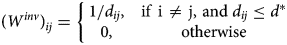
where d ij is the Eucledian distance between two farms i and j and d* is the minimum distance requirement or cut-off. Following Skevas and Grashuis (Reference Skevas and Grashuis2020) and Marasteanu and Jaenicke (Reference Marasteanu and Jaenicke2016), we set d* to the minimum distance that guarantees at least one neighbour to each farmer. The diagonal elements of the inverse distance matrix are set equal to zero since no farm can be viewed as its own neighbor. Finally, following common practice, the inverse distance matrix is scaled by dividing it by its maximum eigenvalue (Elhorst Reference Elhorst2001; Kelejian and Prucha Reference Kelejian and Prucha2010). Note that the inverse distance matrix places a higher weight on closer than more distant neighbors, it is in line with Tobler's First Law of Geography that near units are more likely to be related than distant ones (Tobler Reference Tobler1970), and it is commonly used in studies that examine the role of peer effects in farm decision-making and performance (e.g., Läpple et al. Reference Läpple, Holloway, Lacombe and O'Donoghue2017; Skevas, Skevas, and Swinton Reference Skevas, Skevas and Swinton2018).
The second spatial weights matrix specification, assumes that farmers follow other farmers close to them both geographically and with higher farm profit levels. This matrix is constructed as the Hadamard productFootnote 3 of the inverse distance matrix (before normalization) defined in equation 2 and a time-varying matrix that reflects the economic distance between a given farmer and his/her more economically successful neighborsFootnote 4: $W_t^{inv{\rm \_}s} = W^{inv}\circ W_t^s$ , where
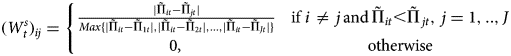
where $\tilde{\Pi }_{it}$ is the inverse hyperbolic sine transformation of profit per cow of farmer i at time t (see section “Results” for the reasoning behind this transformation), | ⋅ | denotes absolute value, and J is the number of observations in the sample less the farm under investigation (i.e., i). In $W_t^s$
 , the absolute difference in profit levels between two farmers i and j is divided by the maximum absolute difference in profit between farmer i and all other farmers in the sample. This procedure allows weights in $W_t^s$
 to range from close to zero (little interaction or influence between two farmers) to one (maximum interaction or influence between two farmers), facilitating influence contrasts between farmer i and his/her more economically successful neighbors. This matrix was then multiplied (in a Hadamard way) by the inverse distance matrix to assure that a higher weight is assigned to the closest (in distance terms) more profitable neighbors. Hence, the final matrix $W_t^{inv{\rm \_}s}$
 assumes that farmers follow other farmers close to them both geographically and with higher profit levels. The latter assumption is motivated by the finding that farmers, both in developing (Conley and Udry Reference Conley and Udry2010) and developed countries (Chatzimichael, Genius, and Tzouvelekas Reference Chatzimichael, Genius and Tzouvelekas2014), tend to imitate the behavior of more successful farmers. Following Elhorst (Reference Elhorst2001) and Kelejian and Prucha (Reference Kelejian and Prucha2010), each element of $W_t^{inv{\rm \_}s}$
 is divided by its largest characteristic root. An example showing how the $W_t^{inv{\rm \_}s}$
 matrix works is provided in the supplementary material.
To the best of our knowledge, the employed approach to construct a spatial weight matrix that captures decision makers' proximity to more economically successful peers (i.e., $W_t^{inv{\rm \_}s}$ ) is novel and no implementations of such a matrix have been identified previously. We note, however, that the use of spatial weights that are based on both geographic contiguity and economic distance (using different economic variables and applied to non-agricultural settings) is not uncommon in applied spatial econometrics analysis (see for e.g., Delgado, Lago-Peñas, and Mayor Reference Delgado, Lago-Peñas and Mayor2018; Qu, Wang, and Lee Reference Qu, Wang and Lee2016).
Endogeneity of the Spatial Economic Weight Matrix
Spatial weight matrices that are based on a theory of distance, such as our inverse distance matrix above, are considered exogenous to any system (Getis Reference Getis2009). When spatial weights are determined by economic variables, such as the profit variable in the case of $W_t^{inv{\rm \_}s}$ above, then the exogeneity assumption of the spatial weight matrix will likely be violated (Qu, Wang, and Lee Reference Qu, Wang and Lee2016). In our case, farm profitability and SCC might be affected by the same time-varying factors, such as hired labor quality, and cleanliness of the housing, bedding, and milking equipment, which are hard to observe or measure. As a result, it is very likely that $W_t^{inv{\rm \_}s}$
 is correlated with the error term in the SCC model, leading to endogeneity bias.Footnote 5
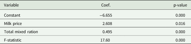
To deal with the potential endogeneity problem, we use a two-stage instrumental variables (2SIV) approach, which was developed by Qu, Wang, and Lee (Reference Qu, Wang and Lee2016). In the first step, we estimate the following regression model:
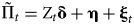
where $\tilde{\Pi }$ is an N × 1 vector of the inverse hyperbolic sine transformation of profits per cow observed in period t, Z is an N × L matrix of instruments, η is an N-dimensional vector of unobserved farm-specific heterogeneity effects,Footnote 6 and ξ is a N-dimensional vector of disturbance terms. The residuals from estimating equation 4 are then included in the following SLX model:

where ϕ is a parameter to be estimated, ut is an N × 1 vector of disturbances, and all other variables are as previously defined. Once ξ has been added in equation 5, the spatial weight matrix could be treated as exogenous (Qu, Wang, and Lee Reference Qu, Wang and Lee2016). This is because the unobserved factors that may affect both the spatial weight matrix and SCC are now captured by ξ, implying that the spatial weight matrix is not anymore correlated with ut. Therefore, we would expect that ξ significantly affects SCC.
Data and Empirical Issues
The data set used in this study was drawn from the Agricultural Financial Advisor (AgFA) database managed by the University of Wisconsin—Madison Center for Dairy Profitability. It is a balancedFootnote 7 panel of 83 specialized dairy farms for the period 2014–2017. These farms are operating in three contiguous counties, namely Sheboygan, Manitowoc, and Kewaunee, which stand out as having by far the highest proportion of farms in the database. Focusing on these counties ensures that each sample farmer has a considerable number of neighboring farmers.Footnote 8
Data available include financial and production information as well as information on the exact location of the dairy farms in the form of farm coordinates. Information on SCC is available at the herd level (herd average) and measured in cells per ml. As explained earlier, SCC is an indicator of mastitis. It is widely accepted that most contagious mastitis is transmitted by fomites (e.g., milkers' hands, the milking unit, and udder wash cloths) from infected to non-infected animals during the milking process. The recommendations to decrease/control mastitis normally include management practices within the farm such as equipment cleaning, proper milking procedure, good beds for the cows, cleanliness of facilities, etc. Our selection of factors (X) that may influence SCC is based on data availability and previous research on determinants of SCC (Dong, Hennessy, and Jensen Reference Dong, Hennessy and Jensen2012; Volpe et al. Reference Volpe, Park, Dong and Jensen2015). These factors include the following: herd size, summer precipitation and temperature, debt-to-asset ratio, non-farm income, and farm subsidies. Herd size is measured by the number of cows in an operation. The summer temperature and precipitation variables were constructed using the Parameter-Elevation Regressions on Independent Slopes Model (PRISM) maps (http://www.prism.oregonstate.edu/). Following Qi, Bravo-Ureta, and Cabrera (Reference Qi, Bravo-Ureta and Cabrera2015), summer in Wisconsin was defined as the months of June through September. Farm coordinates were then used to generate farm-specific average temperature and precipitation for the summer months that a farm is present in the panel. Debt-to-asset ratio is measured as the total debt a farm holds divided by its total assets. Non-farm income is a dummy variable assigned a value of one if the farmer earned income from non-agricultural activities, and zero otherwise. Finally, subsidies include all government payments received by farmers, including those relating to crop and livestock production and conservation. All SCC determinants (X) are used in logarithmic form in equations 1 and 5, except for non-farm income.
The profit per cow variable that is used in the construction of $W_t^{inv{\rm \_}s}$ and in the instrumental variable approach (equation 4) is defined as the value of production less total operating costs and is expressed per livestock unit. Twenty two percent of the observations in our sample have negative profit per cow. To avoid deleting these observations from the analysis, the inverse hyperbolic sine transformation (arcsinh) is used: $\tilde{\Pi }_{it} = arcsinh\lpar {\Pi_{it}} \rpar = ln\left({\Pi_{it} + \sqrt {\Pi_{it}^2 + 1} } \right)$
 .Footnote 9 The instruments used in equation 4 are the natural logarithm of the farm-level milk price and the use of a total mixed ration (TMR) feeding system. Milk price is measured in dollars per hundredweight. TMR is a dummy variable that takes the value of one if a farmer uses TMR to feed his/her cows, and zero otherwise. TMR is normally a long-standing farm decision. Farmers who elected it, will go with it for the foreseeable future. Simple descriptive statistics shows that farmers using TMR do not switch to a non-TMR feeding strategy during the sample period. Therefore, the use of TMR appears unaffected by unobserved factors and stochastic shocks. The employed instruments are assumed to determine farm profitability and, at the same time, have no direct impact on SCC.Footnote 10, Footnote 11
Milk price is a valid instrument because (a) it is not a choice variable and therefore unambiguously exogenous, (b) has a strong and statistically significant effect on farm profitability (Table A1), and (c) it does not have a direct effect on SCC (i.e., it affects SCC only through its effect on farm profitability (e.g., higher milk prices may lead to greater profitability which, in turn, increases a farmer's ability to invest in technologies and practices that reduce SCC)). While SCC levels can affect milk price through premiums and penalties imposed by milk buyers, such an effect is not confirmed in the present study. Correlation analysis revealed an insignificant relationship between SCC and milk price (r = −0.026, p = 0.633). Consistently, linear regression did not show an influence of SCC on milk price (β = −1.408 × 10⁻⁶, p = 0.633).
Note that the employed estimation technique that corrects for the potential endogeneity of $W_t^{inv{\rm \_}s}$ is not a conventional two-stage least squares (2SLS) approach, where the predicted value of the endogenous variable is used in the second-stage model. Under such an approach, and in the event that SCC affects milk price, the predicted value of profit from equation 4 (which would contain the milk price variable) could cause a simultaneity problem when included in equation 5 as an additional explanatory variable. In the contrary, the error term of the first-stage equation (equation 4) is used as an additional explanatory variable in the second-stage model (equation 5) to account for unobserved time-varying factors that might affect both SCC and farm profitability. Hence this procedure as described in Qu, Wang, and Lee (Reference Qu, Wang and Lee2016) provides a valid way of correcting for endogeneity.
Concerning the W inv matrix, the distance cut-off d* was set to 25 km which is the minimum distance that guarantees at least one neighbor to each farmer. To address concerns about the robustness of our results to changes in d*, we estimate models with 35, 45, and 55 km cut-off.
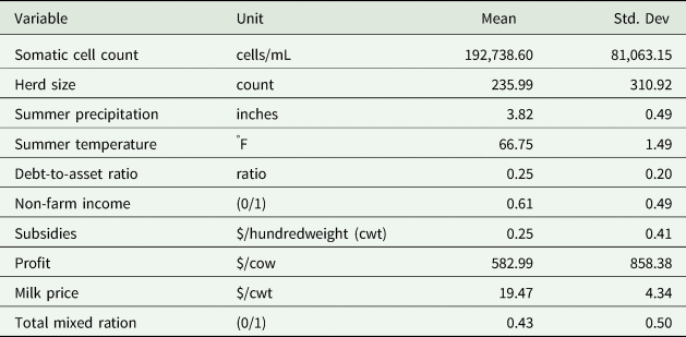
Table 1 presents a summary statistics of the variables used in the analysis. All monetary variables were deflated to 2014 $ using appropriate price indices retrieved from the National Agricultural Statistics Service database.
Table 1. Summary Statistics of the Variables Used in the Analysis
Results
Before we start discussing the results of the empirical models considered in this article, we discuss neighborhood links. Sample farmers have, on average, 29 neighbors within a 25 km radius. On average, the minimum distance to neighboring farmers is 4.2 km, with the shortest distance being 1.1 km. Moving to the results of the estimated models, Table A1 in the appendix reports the first-step estimation results for the 2SIV model. All variables are highly significant with expected signs.Footnote 12 The F-statistic for the joint significance of explanatory variables is greater than 10, confirming that the selected instruments are sufficiently strong (Stock and Watson Reference Stock and Watson2015). Table 2 presents the estimation results from modeling the determinants of SCC. To recall, we estimate and compare three models: (a) a non-spatial OLS model, (b) an SLX model where neighborhood is defined in the dimension of geographic space (hereafter referred to as the SLX-inverse distance), and (c) an SLX model where physical proximity to more profitable farmers is used to capture potential linkages between neighboring farmers (hereafter referred to as the 2SIV-$W^{inv{\rm \_}s}$ ). Since using spatial weight matrices based on different cut-off distances did not change our findings significantly, we present the results from the different spatial models with a 25 km distance cut-off (the remaining results are available from the authors upon request). The results of the Hausman tests suggest that fixed effects estimates are preferred to random effect estimates. Therefore, the results presented in Table 2 are those of the fixed effects models.
Table 2. Regression Results for the Non-spatial and SLX Models
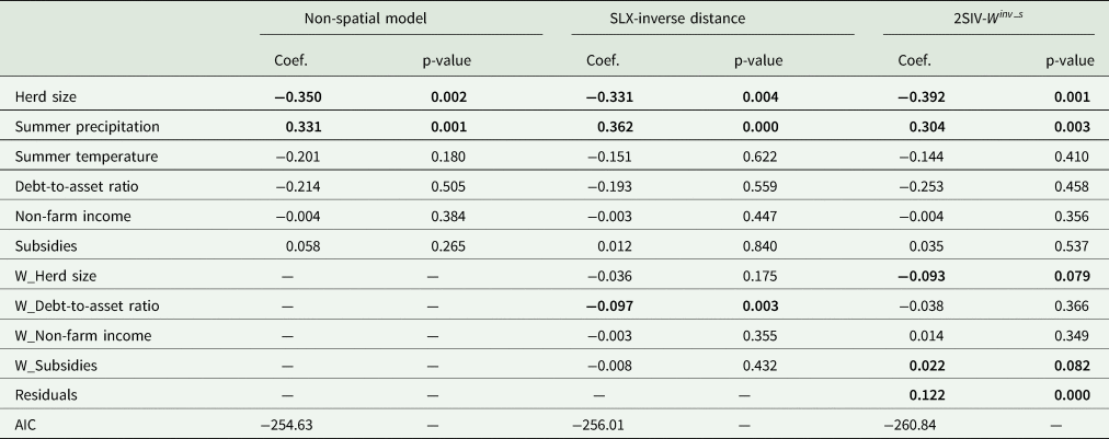
Note: Bold font denotes statistically significant variables. AIC stands for Akaike's Information Criterion. Spatially lagged variables are denoted with a leading “W_”. All continuous variables are in logs.
Notice that the estimated coefficients and their significance levels of the non-spatially lagged variables (upper half of Table 2) do not differ significantly across the different model specifications. Hence, the interpretation of these coefficients applies to all models that are presented in Table 2.
SCC is related significantly to two variables: herd size, and summer precipitation. Larger farms in terms of herd size are found to have lower SCC. More specifically, a 1 percent increase in herd size leads, on average, to a decrease in SCC between 0.33 to 0.39 percent. A reason for this finding may be that larger farms have more expertise in detecting, preventing, and controlling mastitis than smaller farms. Large farms may also have more financial resources to adopt new technologies and farm management practices that can reduce SCC (e.g., milk recording). This result is in line with the studies by Volpe et al. (Reference Volpe, Park, Dong and Jensen2015) and Oleggini, Ely, and Smith (Reference Oleggini, Ely and Smith2001) who found a negative relationship between herd size and SCC in U.S. dairy farming. An increase in precipitation during the summer months is found to increase SCC. Increased summer rainfall contributes to high humidity which is known to be related to mastitis infection (Morse et al. Reference Morse, DeLorenzo, Wilcox, Collier, Natzke and Bray1988).
We now turn to the interpretation of the effect of the spatially lagged explanatory variables on SCC (lower half of Table 2).Footnote 13 Both spatial models include statistically significant spatially lagged covariates, implying that peer effects do play a role in explaining farm-level SCC. There are, however, differences across the employed spatial models in terms of the significance of peer effects. As expected, and in line with previous research (Läpple and Kelley Reference Läpple and Kelley2015; Mourao Reference Mourao2019) indirect effects (i.e., the coefficients of the spatially lagged variables) are smaller in magnitude than the respective direct effect estimates. This is because they reflect cumulative spillovers from all farmers within the distance cut-off.Footnote 14
Of the spatially lagged variables included in the SLX-inverse distance model, only debt-to-asset ratio is found to be a statistically significant predictor of SCC. More specifically, a (cumulative) 1 percent increase in neighboring farmers' debt-to-asset ratio decreases SCC by about 0.1 percent. This implies that farmers that have more indebted neighbors have cows with lower SCC. Highly indebted farms may have recently invested in management practices and technologies that decrease SCC. Nearby farmers may learn from these investments, and adopt similar technologies on their own farms.
Regarding the spatially lagged variables of the 2SIV-$W^{inv{\rm \_}s}$ model, two were found to be significant predictors of SCC: herd size, and subsidies. The spatial lag of the herd size variable has a negative effect on SCC. More specifically, a (cumulative) 1 percent increase in neighbors' herd size decreases SCC by about 0.1 percent, likely pointing to the existence of a learning effect between large farms and their neighbors. Large farms have more resources at their disposal to invest in new technologies and management practices that reduce SCC. Nearby farmers could learn about the effectiveness of these new technologies and practices in reducing SCC, for example, by communicating with their neighbors, and modifying their strategies accordingly to better deal with mastitis prevention and control. More studies in the literature report the existence of spatial spillovers between large farmers and their neighbors (Läpple et al. Reference Läpple, Holloway, Lacombe and O'Donoghue2017; Storm, Mittenzwei, and Heckelei Reference Storm, Mittenzwei and Heckelei2014). Note that unlike in the 2SIV-$W^{inv{\rm \_}s}$
 model, the spatially lagged herd size variable is statistically insignificant in the SLX-inverse distance model. An explanation for this difference may be that neighboring large farmers (in terms of herd size) are not necessarily the most efficient ones in reducing mastitis. Reduced mastitis incidence should be reflected in higher farm profitability as it often entails lower production costs and milk price bonuses. Therefore, the largest and at the same time more profitable farms are expected to have lower SCC and exert a greater influence on neighboring farms than large farms alone. Indeed, a closer look of the data shows that the top 25 percent of the largest farms (in terms of herd size) in our sample have, on average, 10 percent higher SCC scores than the top 25 percent of the most profitable farms in the same subset of largest farms. Moving to the interpretation of the spatially lagged subsidy variable, farmers surrounded by neighboring peers that receive high subsidy income are found to have cows with higher SCC. High subsidies may induce farmers to substitute farm income with subsidy income and expend less effort in implementing management practices that lower the incidence and severity of mastitis. Nearby farmers may mimic their neighbors' behavior and experience increases in mastitis incidence. Finally, the residuals from the first-step estimation are significant at the 1 percent level, giving strong support that farm profitability is the source of the endogeneity of the $W_t^{inv{\rm \_}s}$
 matrix.
Finally, among all the employed models, the AIC (bottom of Table 2) favors the 2SIV-$W^{inv{\rm \_}s}$ model. That is, the data favor the model in which spatial effects are defined in terms of both geographic proximity and farm profitability.
Conclusions
Using a panel dataset of 83 Wisconsin dairy farms over the period 2014–2017, this article examines the factors influencing average herd somatic cell count (SCC). We specifically explore whether and to what extent spatial spillovers affect SCC, making it the first article to link SCC with peer influence. Moreover, unlike previous studies that examine the role of spatial spillovers on farm decision-making and performance, we examine whether defining the neighborhood space both in terms of physical proximity and farm profitability gives rise to spatial spillovers.
The findings from this article indicate that SCC is not only affected by own-farm decisions and characteristics but also by those of neighboring farms. This result implies that future work aiming at exploring the determinants of SCC should test for and, if necessary, account for peer effects to make accurate inferences. We also find that farm profitability is an important driver of spatial spillovers among neighboring farms. Significant differences in the estimated spatial spillovers are observed when using farm profitability as well as physical proximity to define the neighborhood links, as opposed to using just physical proximity. Model comparison results show that defining the neighborhood space in terms of proximity to more profitable peers (as compared to physical proximity alone) improves model fit. One should keep in mind, however, that this result is case-specific. The construction of spatial weight matrices is an open and debatable question, and must be guided by theoretical considerations and represent as far as possible real social and economic phenomena (Corrado and Fingleton Reference Corrado and Fingleton2012). What can be learned from this article is that researchers should be aware that the choice of the spatial weight matrix can have a strong effect on the inferences made in regard to the effect of spatial spillovers on the variable of interest.
Results also provide useful clues about the channels through which spatial spillovers operate. These channels are: (a) neighboring large farmers, and (b) indirect effects of neighboring farmers' financial characteristics such as subsidies received. It is likely that these channels arise as a result of direct communication or influence between neighboring farmers on farm practices and decision-making. For example larger farms are often more likely to adopt agricultural innovations in order to reduce the occurrence of mastitis. Neighboring farmers may adopt similar technologies either because they interact with, and learn from large neighbors or from a desire to conform with peers' choices. Previous studies indeed show that Wisconsin dairy farms influence each other in decisions to adopt new practices (Lewis, Barham, and Robinson Reference Lewis, Barham and Robinson2011).
Apart from spatial spillovers, this article also shows that direct (i.e., own-farm) effects affect SCC. More specifically, farmers operating large farms (in terms of herd size) are found to have cows with lower SCC. On the other hand, higher summer precipitation leads to an increase in SCC.
Considered together, these results provide direct and indirect paths for lowering farm-level SCC. In relation to direct paths, the presence of peer effects in the context of mastitis management imply potentially large social multiplier effects and economic gains related to reduced SCC through exchange of information between neighboring farmers on good management practices to control and prevent mastitis. Hence, strategies that promote peer interactions and learning effects might prove efficacious in reducing farm-level SCC. Such strategies may include field days, farm walks on farms that are efficient in reducing SCC, and discussion meetings. Regarding indirect paths, the fact that larger farms have lower SCC, and this positively impacts neighboring farms efforts to reduce SCC, implies that the generally observed trend in U.S. dairy sector of expanding and intensifying production may trigger further decreases in mastitis incidence and related economic losses.
Finally, while our findings provide quantitative support for the presence of spatial spillovers on neighboring farms' SCC and allow for judgments to be made regarding the channels through which these effects operate, further work is needed to provide behavioral insights of how these spillovers arise and if farmer-to-farmer information transfers and exchanges do happen in practice. Further work could also examine whether spatial spillovers arise as result of physical proximity to farmers of a similar income level. Such farmers may influence each other's behavior because they are likely to face comparable budget constraints and tackle similar problems.
Supplementary material
The supplementary material for this article can be found at https://doi.org/10.1017/age.2020.22
Acknowledgments
The authors wish to thank the Center for Dairy Profitability at the University of Wisconsin-Madison and its Associate Director, Jenny Vanderlin, for providing the data and for useful discussions.
Conflicts of Interest
None.
Appendix
Table A1. Empirical Results for the First Stage of the 2SIV Approach


 Open access