


Introduction
Enrollment in the federal crop insurance program is rising, which raises concerns about the effects of crop insurance on farm production decisions. Crop acres insured by this program tripled in the last three decades with almost 300 million acres insured in 2018 Footnote 1 . Quiggin, Karagiannis, and Stanton (Reference Quiggin, Karagiannis and Stanton1994) argue that moral hazard in crop insurance increases the “severity of loss” once farms are insured. Annan and Schlenker (Reference Annan and Schlenker2015) suggest that the incentives of the insured farms to adapt to extreme weather events may diminish in the presence of subsidized crop insurance. In the farm input use context, moral hazard leads to a farm applying less risk-reducing or applying more risk-enhancing farm inputs once they are insured.
There has been debate on whether a farm input is risk-increasing or risk-decreasing. Quiggin, Karagiannis, and Stanton (Reference Quiggin, Karagiannis and Stanton1993) mention that “pesticides are generally viewed as a risk-reducing input and fertilizer as a risk-increasing input.” Horowitz and Lichtenberg (Reference Horowitz and Lichtenberg1993) argue that both pesticides (herbicides and insecticides) and nitrogen are likely to be risk-increasing inputs. This argument may seem counterintuitive for farm producers. But, according to Horowitz and Lichtenberg (Reference Horowitz and Lichtenberg1993), “an input increases risk if it adds relatively more to output in good states than in bad ones, since that increases the discrepancy among states.” Babcock and Hennessy (Reference Babcock and Hennessy1996) find the results of Horowitz and Lichtenberg (Reference Horowitz and Lichtenberg1993), particularly associated with pesticides, “somewhat surprising.” Babcock and Hennessy (Reference Babcock and Hennessy1996) argue that increased pesticides should result in a decreased probability of low yield because, unlike fertilizer, pesticides do not directly affect yield. Though there is more possibility of fertilizer being risk-increasing and pesticides being risk-decreasing input, an input could be both risk-decreasing and risk-increasing at different levels of application (Babcock and Hennessy, Reference Babcock and Hennessy1996).
Mixed evidence exists regarding crop insurance moral hazard effects on farm input use. Some previous studies find that crop insurance encourages farmers to apply more farm chemicals. Using farm-level cross-sectional data, Horowitz and Lichtenberg (Reference Horowitz and Lichtenberg1993) find that insured farms apply 19% more nitrogen, apply 7% more herbicides, apply 21% more insecticides, and spend 21% more on pesticides per acre than uninsured farms. Similarly, Wu (Reference Wu1999) examines USDA’s Areas Studies data for the Central Nebraska Basins and finds that crop insurance increases farm chemical use by encouraging farms to shift towards more input-demanding crops.
In contrast, other studies find that crop insurance reduces farm chemical usage. Smith and Goodwin (Reference Smith and Goodwin1996) argue that Horowitz and Lichtenberg (Reference Horowitz and Lichtenberg1993) ignored simultaneity between crop insurance purchase decision and farm input use. Using Kansas Farm Management Association data for dryland-wheat producers and accounting simultaneity using Amemiya’s two-step estimator, Smith and Goodwin (Reference Smith and Goodwin1996) find that insured farms spend $4.23 less per acre on fertilizer than uninsured farms. Goodwin, Vandeveer, and Deal (Reference Goodwin, Vandeveer and Deal2004) examine both farm chemical use and crop acreage response to insurance in a structural equation framework using pooled cross-sectional and time-series data. Goodwin, Vandeveer, and Deal (Reference Goodwin, Vandeveer and Deal2004) find that increased crop insurance participation likely decreases fertilizer and chemical expenditures per acre for wheat and barley though it leads to a modest increase in crop acreage.
Though results of crop insurance effects on farm input use are mixed, most of these studies published several years ago do not consider empirically that the crop insurance purchase decision may be correlated with farm-level unobserved heterogeneity. A more recent study accounting for farm-level heterogeneity finds a small positive effect of crop insurance coverage on farm chemicals usage (Weber, Key, and O’Donoghue, Reference Weber, Key and O’Donoghue2016). However, Weber, Key, and O’Donoghue (Reference Weber, Key and O’Donoghue2016) do not estimate the difference in farm chemical usage between insured and uninsured farms.
The objective of this research is to examine the effects of a change in crop insurance coverage separately from a change in crop insurance enrollment on farm input use decisions using recent data accounting for farm-level heterogeneity. Unlike many previous studies that use county-level aggregates of farm production decisions, this study uses farm-level data from Kansas. County-level aggregates may mask variation at the farm level. The data used in this study provide an opportunity to exploit farm-level variation on input use and crop insurance purchase decisions in an unbalanced panel framework.
Overall, this study estimates the effects of crop insurance on farm input use after controlling for unobserved heterogeneity at the farm level. First, we estimate the effects of crop insurance purchase on the use of three farm inputs (fertilizer, agrochemicals, and seed) Footnote 2 . Second, we estimate the effects of a change in crop insurance coverage on farm input use. The research uses a fixed effects model and a quasi-experimental design to estimate the effects of crop insurance participation on farm input use. The effects of crop insurance coverage level on farm input use are estimated using a fixed effects instrumental variable estimator (Weber, Key, and O’Donoghue, Reference Weber, Key and O’Donoghue2016). This research finds that insured farms purchase more farm inputs than uninsured farms. However, a statistically significant effect of the change in the crop insurance coverage level on farm chemical use was not found.
Conceptual framework
This paper aims to estimate the effects on farm input use from the purchase of crop insurance and a change in the insurance coverage level by those that have purchased crop insurance.
A profit function for a farm can be generalized as:
 $$\pi = py - wx$$
where py and wx represent total gross revenue (r) and total cost at output price p and input price w. Farmer’s choose input level x to maximize $E[U(\pi )]$
. The first-order condition is:
$E[U(\pi )]$
. The first-order condition is:
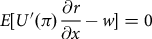 $$E[U^\prime(\pi ){\partial r \over \partial x} - w]\,\!=\,\!0$$
Quiggin, Karagiannis, and Stanton (Reference Quiggin, Karagiannis and Stanton1994) suggest for a guaranteed yield ${y^*}$
at election price
${y^*}$
at election price ${p^*}$
with total premium (
${p^*}$
with total premium ( $\psi $
), crop insurance modifies the total revenue
$\psi $
), crop insurance modifies the total revenue $({r^m})$
such that:
$({r^m})$
such that:
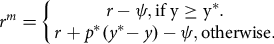 $${r^m} = \!\left\{ \matrix{{r - \psi ,{\rm{if}}\,{\rm{y}} \ge {{\rm{y}}^{\rm{*}}}.}\cr {r + {p^*}({y^*} \!- y) - \psi ,{\rm{otherwise}}.}} \right.$$
The total benefit ( $\tau $
) from crop insurance enrollment is represented as:
$\tau $
) from crop insurance enrollment is represented as:
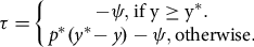 $$\tau = \!\left\{ \matrix{{ - \psi ,{\rm{if \, y}} \ge {{\rm{y}}^{\rm{*}}}.}\cr{{p^*}({y^*}\! - y) - \psi ,{\rm{otherwise}}.}} \right.$$
Assuming $f(y|x)$
is the probability density function for y, the marginal revenue product for inputs is the input demand:
$f(y|x)$
is the probability density function for y, the marginal revenue product for inputs is the input demand:
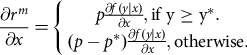 $${{\partial {r^m} \over \partial x}} = \!\left\{ \matrix{{p{{\partial f(y|x) \over \partial x}},{\rm{if\, y}} \ge {{\rm{y}}^{\rm{*}}}.}\cr{(p - {p^*}){{\partial f(y|x) \over \partial x}},{\rm{otherwise}}.}} \right.$$
Equation (5) can also help to understand the moral hazard incentives associated with crop insurance enrollment. For example, a risk-neutral producer would have an incentive to apply more fertilizer than required so that the likelihood of low yield decreases. A similar incentive for farm chemical application exists in the revenue protection program to reduce the likelihood of low revenue. Next, we provide a discussion of crop insurance coverage and farm input use under revenue protection.
The Babcock and Hennessy (Reference Babcock and Hennessy1996) approach is used to determine the economic relationship between crop insurance coverage and farm input use. At the insured revenue level ${r^*}$
, the producer chooses the input level x to maximize expected utility:
${r^*}$
, the producer chooses the input level x to maximize expected utility:
 $$Ma{x_x}EU \!= \!\int_2 U({\pi _{{r}^*}})g(p)f(y|x)dz + \int_{{2^\prime}} U({\pi _{py}})g(p)f(y|x)dz$$
where $U(.)$
is the utility function,
$U(.)$
is the utility function, ${\pi _r} \!= {r^*} \!- wx$
and
${\pi _r} \!= {r^*} \!- wx$
and ${\pi _{py}} \!= py - wx$
are profit functions for per unit input price w and per unit output price p. The probability density function for output price is
${\pi _{py}} \!= py - wx$
are profit functions for per unit input price w and per unit output price p. The probability density function for output price is $g(p)$
and
$g(p)$
and $f(y|x)$
is the probability density function for yield (y) conditional on x. The brevity of integrals follows Mieno, Walters, and Fulginiti (Reference Mieno, Walters and Fulginiti2018), for a yield level y ranging between i and j (
$f(y|x)$
is the probability density function for yield (y) conditional on x. The brevity of integrals follows Mieno, Walters, and Fulginiti (Reference Mieno, Walters and Fulginiti2018), for a yield level y ranging between i and j ( $i \le y \le j$
),
$i \le y \le j$
), $\int_2 $
represents two integrals
$\int_2 $
represents two integrals $\int_0^\infty \int_i^{{r^*}/p} $
, similarly
$\int_0^\infty \int_i^{{r^*}/p} $
, similarly $\int_{{2^\prime}} $
represents two integrals
$\int_{{2^\prime}} $
represents two integrals $\int_0^\infty \int_{{r^*}/p}^j $
, and dz represents
$\int_0^\infty \int_{{r^*}/p}^j $
, and dz represents $dydp$
.
$dydp$
.
The first-order condition (FOC) is:
 $$\begin{align*}&{{\partial EU(\pi ) \over \partial x}} = \int_2 U({\pi _{{r^*}}})g(p){{\partial f(y|x) \over \partial x}}dz - w{U^{'}}({\pi _{{r^*}}})g(p)f(y|x)dz\\
&\quad + \int_{{2^{'}}} \!U({\pi _{py}})g(p){{\partial f(y|x) \over \partial x}}dz - w{U^{'}}({\pi _{py}})g(p)f(y|x)dz = \!0\end{align*}$$
$$\begin{align*}&{{\partial EU(\pi ) \over \partial x}} = \int_2 U({\pi _{{r^*}}})g(p){{\partial f(y|x) \over \partial x}}dz - w{U^{'}}({\pi _{{r^*}}})g(p)f(y|x)dz\\
&\quad + \int_{{2^{'}}} \!U({\pi _{py}})g(p){{\partial f(y|x) \over \partial x}}dz - w{U^{'}}({\pi _{py}})g(p)f(y|x)dz = \!0\end{align*}$$
The quantity of interest is the marginal impact of a change in revenue coverage on input use [ ${{\partial x \over \partial {r^*}}}$
]. Babcock and Hennessy (Reference Babcock and Hennessy1996) indicate that revenue is an implicit function of input use, and the comparative statistics are obtained by differentiating the FOC with respect to x and
${{\partial x \over \partial {r^*}}}$
]. Babcock and Hennessy (Reference Babcock and Hennessy1996) indicate that revenue is an implicit function of input use, and the comparative statistics are obtained by differentiating the FOC with respect to x and ${r^*}$
as:
${r^*}$
as:
 $${{\partial x \over \partial {r^*}}} = - {\left[ {{{{\partial ^2}EU(\pi ) \over \partial {x^2}}}} \right]^{ - 1}}\left[ {{U^{'}}({\pi _{{r^*}}})\int_2 g(p){{\partial f(y|x) \over \partial x}}dz - w{U^{''}}({\pi _{{r^*}}})\int_2 g(p)f(y|x)dz} \right] $$
Using Leibniz’s rule and rearranging terms (Babcock and Hennessy, Reference Babcock and Hennessy1996):
 $${{\partial x \over \partial {r^*}}} = - {\left[ {{{{\partial ^2}EU(\pi ) \over \partial {x^2}}}} \right]^{ - 1}}{U^{'}}({\pi _{{r^*}}})\int_2 h(p)f(y|x)dz\left[ {{{d\;log\left\{ {\int_2 g(p)f(y|x)dz} \right\} \over dx}} - w {{{U^{''}}({\pi _{{r^*}}}) \over {U^{'}}({\pi _{{r^*}}})}}} \right]$$
Equation (9) indicates the potential effects of crop insurance coverage on farm input use. In equation (9), the outside term, $ - {\left[ {{{{\partial ^2}EU(\pi ) \over \partial {x^2}}}} \right]^{ - 1}}{U^{'}}({\pi _{{r^*}}})\int_2 h(p)f(y|x)dz $
, is positive because
$ - {\left[ {{{{\partial ^2}EU(\pi ) \over \partial {x^2}}}} \right]^{ - 1}}{U^{'}}({\pi _{{r^*}}})\int_2 h(p)f(y|x)dz $
, is positive because ${\left[ {{{{\partial ^2}EU(\pi ) \over \partial {x^2}}}} \right]^{ - 1}}$
is a second-order condition that is assumed to be negative. The first term inside the second bracket,
${\left[ {{{{\partial ^2}EU(\pi ) \over \partial {x^2}}}} \right]^{ - 1}}$
is a second-order condition that is assumed to be negative. The first term inside the second bracket, ${{d\;log\left\{ {\int_2 g(p)f(y|x)dz} \right\} \over dx}}$
, represents a change in probability of indemnity payment due to a per unit change in input use that is positive (negative) if an input increases (decreases) the probability of making claim. The second term inside the same bracket,
${{d\;log\left\{ {\int_2 g(p)f(y|x)dz} \right\} \over dx}}$
, represents a change in probability of indemnity payment due to a per unit change in input use that is positive (negative) if an input increases (decreases) the probability of making claim. The second term inside the same bracket, $ - w{{{U^{''}}({\pi _{{r^*}}}) \over {U^{'}}({\pi _{{r^*}}})}}$
, is positive under risk aversion. The right-hand side of equation 9 suggests that the risk preferences of farmers and the riskiness of inputs shape the relationship between changes in crop insurance coverage and farm input use.
$ - w{{{U^{''}}({\pi _{{r^*}}}) \over {U^{'}}({\pi _{{r^*}}})}}$
, is positive under risk aversion. The right-hand side of equation 9 suggests that the risk preferences of farmers and the riskiness of inputs shape the relationship between changes in crop insurance coverage and farm input use.
This theoretical framework could be used to discuss the production behavior, particularly input use decisions, of producers with different levels of riskiness. It also accounts that the same input could both increase and decrease the probability of making a claim at different levels of its application. The riskiness of farm producers generally falls in the range of risk-neutral to moderately risk averse (Abdulkadri, Langemeier, and Featherstone, Reference Abdulkadri, Langemeier and Featherstone2003). Under risk aversion, equation (9) would be positive only if the input is risk-increasing. Since the same input could be both risk-increasing and risk-decreasing at different levels of application (Babcock and Hennessy, Reference Babcock and Hennessy1996), it is challenging to assign a sign of equation (9) only based on producers’ risk aversion levels.
Data
We obtain a farm-level unbalanced panel from the Kansas Farm Management Association (KFMA). KFMA data are “representative of commercial farming operations in Kansas” (Goodwin and Kastens, Reference Goodwin and Kastens1996). KFMA is “one of the largest management programs in the USA” (Kuethe et al., Reference Kuethe, Briggeman, Paulson and Katchova2014). KFMA consists of six regional associations that maintain historical Kansas farm-level information. These data provide information on farming practices and financial outcomes of farms enrolled in the KFMA Footnote 3 . KFMA data are representative of the USDA Agricultural Resource Management Survey (ARMS) but with a relatively larger farm size, a higher share of crop acreage, and younger operators (Kuethe et al., Reference Kuethe, Briggeman, Paulson and Katchova2014).
The sample ranges from 1993 through 2016 and consists of 30,187 observations. Figure 1 shows the trend of crop insurance participation among the sample observations. There is a jump in crop insurance participation after 1993 to 1996, a slight drop from 1996 to 1999, and relatively stable but high participation after that. For example, the proportion of insured farms is in excess of 75% of farms in 2016 in the final estimation sample.
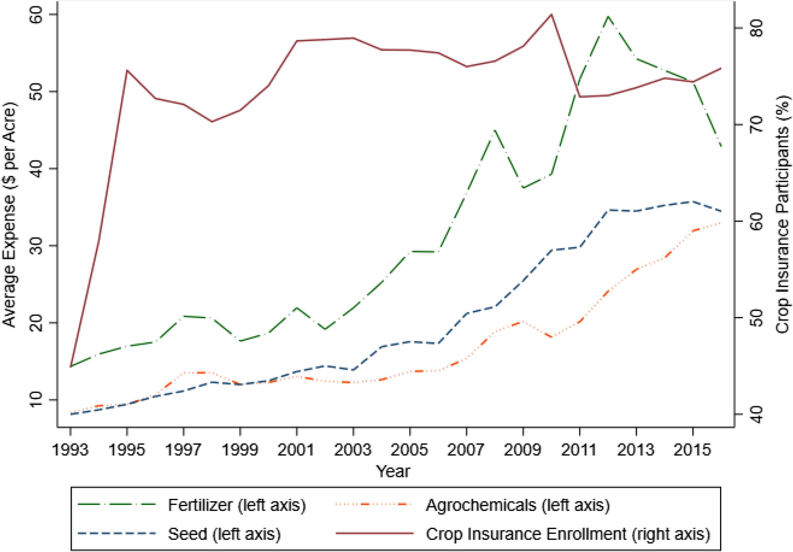
Figure 1. Farm input expenditures per acre and crop insurance enrollment in Kansas.
Notes: The term “fertilizer” represents fertilizer and lime expenditures per acre, “agrochemicals” represents herbicides and insecticides expenditures per acre, and “seed” represents “seed and other crop” expenditures per acre.
Data Source: Kansas Farm Management Association.
The mean expenditures on fertilizer, agrochemicals, and seed are $21.96 per acre, $11.60 per acre, and $12.26 per acre, respectively (Table 1). The respective average acres under wheat, corn, and soybeans are 29.8%, 9.7%, and 17.2%. Non-irrigated acreage is 94.5% of total acres. The sample average of value of farm production is $217,242, net farm income is $42,240, and non-farm income is $19,837. Average age of the operator is 54 years.
Table 1. Summary statistics of farm characteristics, crop production, income, farm input expenses, crop insurance expenses, and financial indicators in Kansas
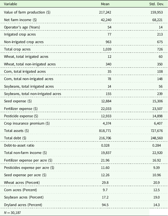
Data Source: Kansas Farm Management Association.
There is an increasing trend in fertilizer, agrochemical, and seed expenditures from 1993 to 2016 in nominal dollars (Figure 1). The mean expenditures per acre on fertilizer are larger than agrochemicals and seed throughout the sample period. Average expenditures per acre on agrochemicals are higher than the mean seed expenses per acre after 2001. The average farm expenditures from 1993 to 2016 increased from $14.34 to $42.86 per acre for fertilizer, $8.38 to $32.97 per acre for agrochemicals, and $8.14 to $34.47 per acre for seed.
Crop insurance use in Kansas
KFMA data report annual premium payments but do not report details about insurance products, coverage levels, or insured crop acres. We collect data from two other sources to provide more detail about crop insurance use among farmers in Kansas. Data on insured acres by crop insurance products and coverage level were obtained from USDA Risk Management Agency (RMA). Using total corn-planted acres in 2020 obtained from USDA NASS (National Agricultural Statistics Survey), the percent insured is calculated across insurance products and coverage levels.
Figure 2 depicts the total crop insurance premium, indemnities, insured acres over time in Kansas. There was an increasing trend in federally insured acres in Kansas; about 6.5 million acres, 16.8 million acres, 16.0 million acres, 16.5 million acres, and 18.8 million acres were insured, respectively in 1989, 1995, 2001, 2008, and 2014. A large increase in crop-insured acres in Kansas since 2000 was due to changes in crop insurance policies. The benefits from the federal government and the availability of multiple insurance options have increased farm household crop insurance participation. In particular, the Agricultural Risk Protection Act of 2000 codified previous ad hoc premium reductions into law that led to an increase in subsidy rates for more insurance plans, particularly at higher coverage levels (O’Donoghue, Reference O’Donoghue2014; Yu, Smith, and Sumner, Reference Yu, Smith and Sumner2018). The 2008 Farm Bill increased the enterprise unit premium subsidies but reduced the subsidy rates for area-based products (O’Donoghue, Reference O’Donoghue2014; Yu, Smith, and Sumner, Reference Yu, Smith and Sumner2018). The Risk Management Agency (RMA) of USDA also adjusted premiums for different crops in some regions in 2012 (Shields, Reference Shields2015). The sharp increase in indemnities in 2012 (see Figure 2) was due to a major drought that resulted in a large crop loss (Shields, Reference Shields2015). Acres insured remained fairly stable in Kansas since 2014. The 2014 Farm Bill replaced “support based on historical production” with “shallow loss programs” to cover some of the deductibles (O’Donoghue, Reference O’Donoghue2014).
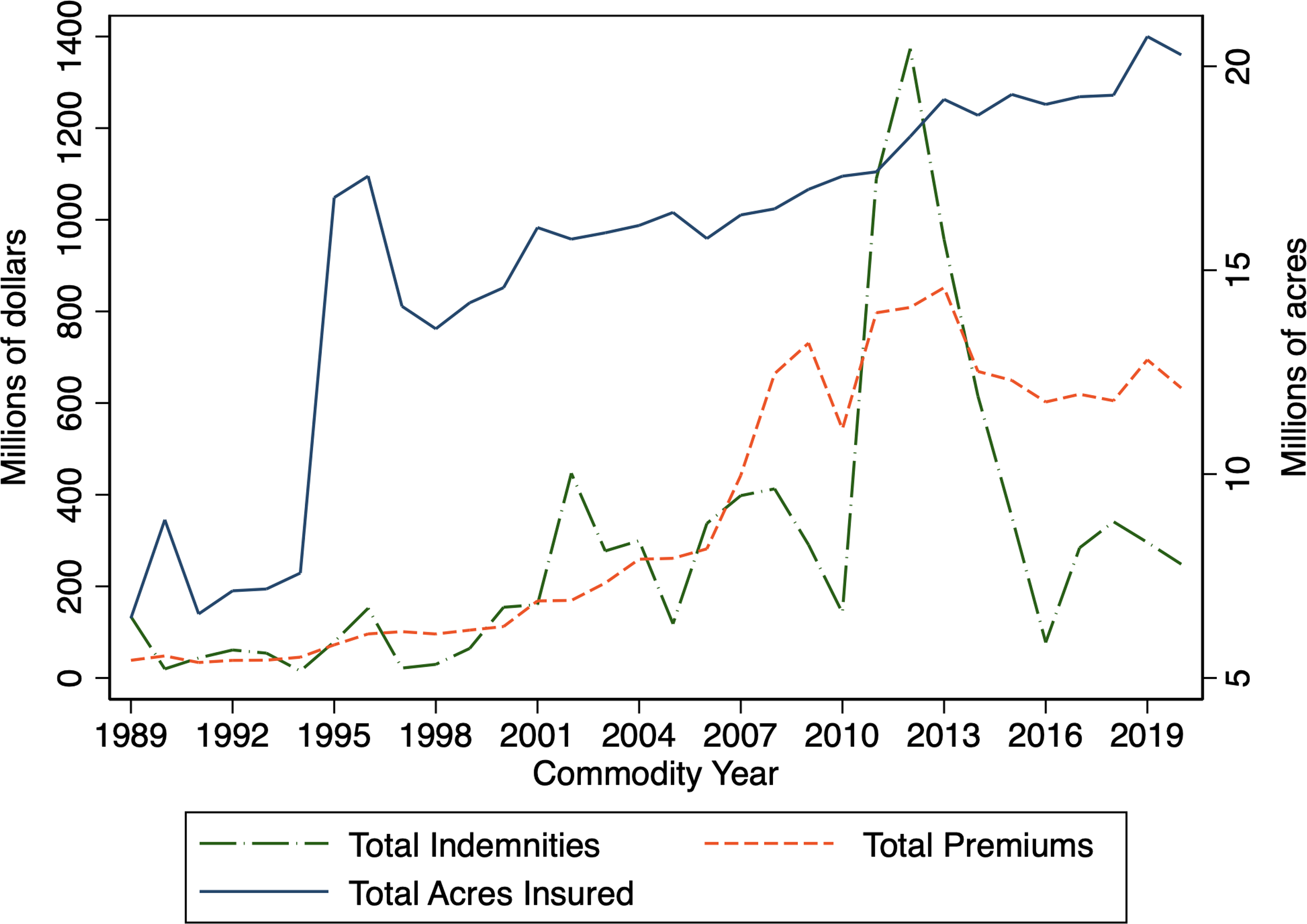
Figure 2. Trends of premiums, indemnities, and acres insured in Kansas.
Data Source: Risk Management Agency (RMA), USDA.
Figure 2 indicates that acres insured remained between 18.3 million acres and 20.7 million acres since 2012. Following the trend of insured acres, total premiums also increased in the first two decades since 1989. The total indemnities (premiums) in Kansas were $134.0 million ($38.7 million), $446.8 million ($169.3 million), $290.8 million ($730.9 million), $1,373.2 million ($808.7 million), and $248.4 million ($632.9 million), respectively in 1989, 2002, 2009, 2012, and 2020. The premiums and indemnities per enrolled acres in Kansas in 2020 were $31.21 and $12.25, respectively.
Figure 3 displays the total premium paid for four major crops (corn, soybean, sorghum, wheat) over time in Kansas. The total premium for all four crops was generally low during the first decade since 1989 but increased in the next decade. The largest total premium was paid for wheat before 2015 but was almost the same for corn ($197.6 million) and wheat ($199.9 million) in 2016. The total premium for corn surpassed wheat after 2017. Total premium in 2020 was $259.1 million, $130.3 million, $199.8 million, and $86.6 million, respectively, for corn, wheat, soybeans, and sorghum.
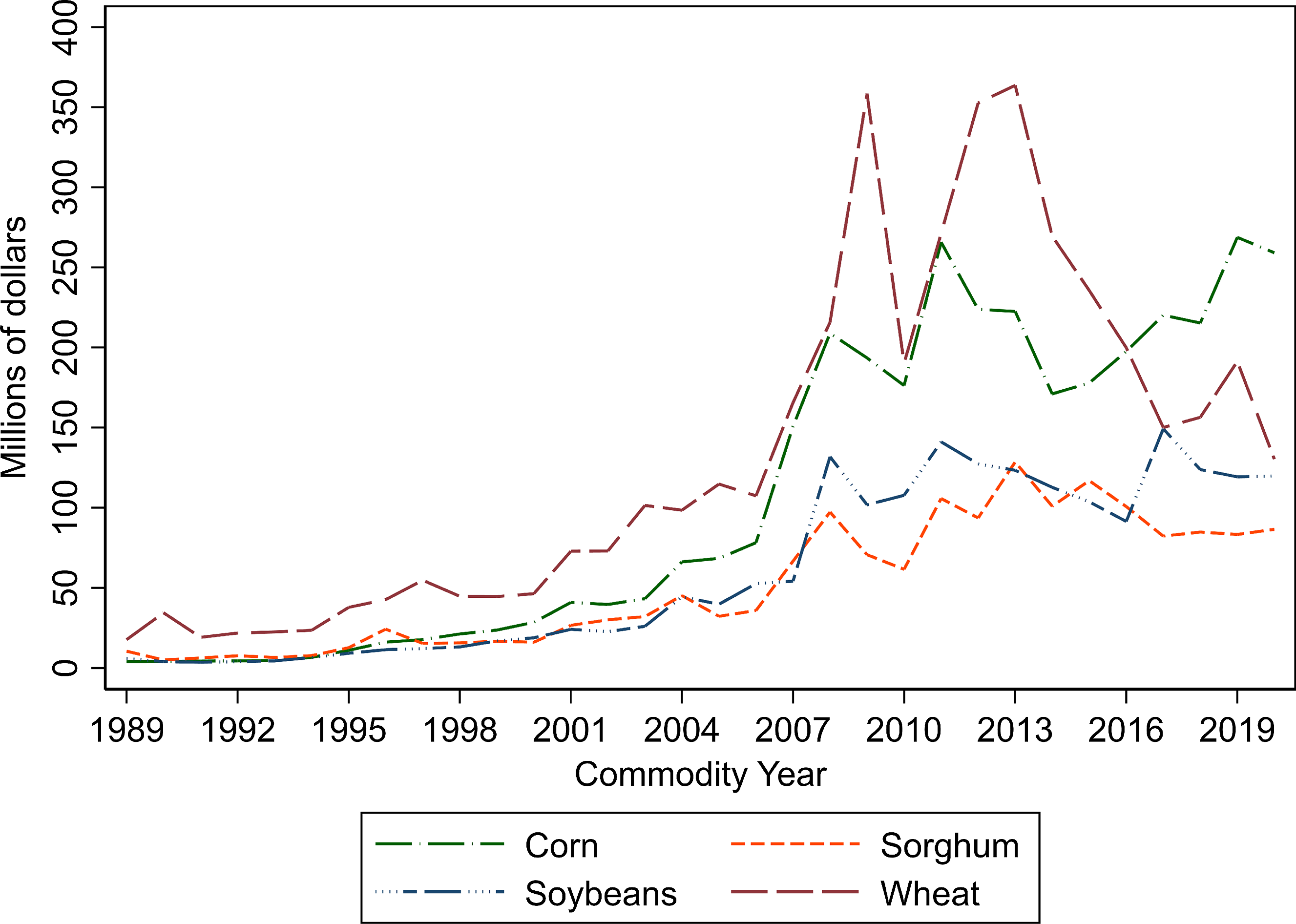
Figure 3. Trends of premiums for major crops in Kansas.
Data Source: Risk Management Agency (RMA), USDA.
Figure 4 shows the share of acres insured by each federal crop insurance product in 2020 in Kansas. The revenue protection (RP) plan is dominant in Kansas accounting for 85.2% of insured acres. The rest of the crop insurance policies such as RI (Rainfall Index), YP (Yield Protection), and others, respectively, accounted 9.4%, 4.8%, and 0.6% of insured acres in 2020.
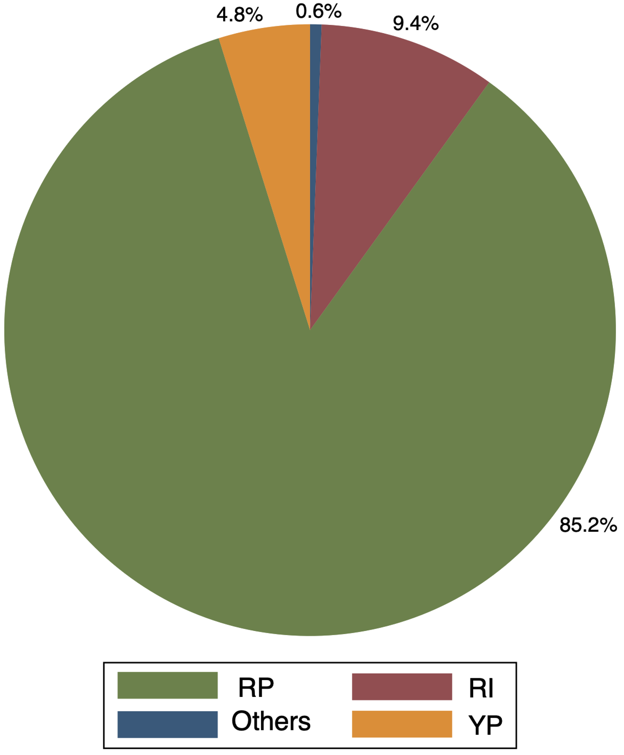
Figure 4. Shares of 2020 insured acres by products in Kansas.
Notes: Three major insurance plans in 2020 are Revenue Protection (RP), Rainfall Index (RI), and Yield Protection (YP).
Data Source: Risk Management Agency (RMA), USDA.
Table 2 presents the percent of corn acres insured Footnote 4 for each federal crop insurance policy in Kansas in 2020. About 94.1% of corn-planted acres were insured in Kansas in 2020 with RP being the highest purchased product (89.8% of insured corn acres) followed by YP (3.9% of insured corn acres). Table 2 shows that the two most popular coverage levels for corn production in 2020 are 75% and 70%, respectively, accounting for 37.3% and 31% of insured corn acres under RP.
Table 2. Percent of corn acres insured by crop insurance policies in Kansas in 2020
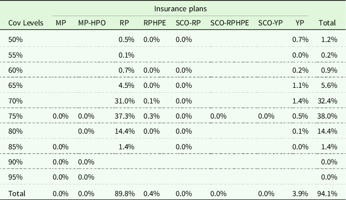
Notes: The insurance plans include Marginal Protection (MP), Marginal Protection with Harvest Price Option (MP-HPO), Revenue Protection (RP), RP with Harvest Price Exclusion (RPHPE), Supplemental Coverage Option for RP (SCO-RP), Supplemental Coverage Option for RPHE (SCO-RPHE), Supplemental Coverage Option for YP (SCO-YP), Yield Protection (YP).
Data Source: National Agricultural Statistics Service (NASS) and Risk Management Agency (RMA), USDA.
Identification strategy
We use a quasi-experimental design and a fixed effect estimator to estimate the effects of crop insurance enrollment on farm input use. The fixed effects instrumental variable estimator measures the effects on farm input use from a change in the insurance coverage level.
Matching
The quantity of interest is the average treatment effect of crop insurance participation on insured farms’ input use (ATT). The ATT for the potential outcome framework is:
 $$ATT \!= \!E(I{N_{i1}}|C{I_i}\!=\!1) - E(I{N_{i0}}|C{I_i}\!=\!1)$$
where $C{I_i}$
is the treatment variable for farm i [takes value of 1 for insured farms and 0 for uninsured farms].
$C{I_i}$
is the treatment variable for farm i [takes value of 1 for insured farms and 0 for uninsured farms]. $E(I{N_{i1}}|C{I_i}\!=\!1)$
is the mean farm input expenditures per acre (IN) for insured farm, subscript
$E(I{N_{i1}}|C{I_i}\!=\!1)$
is the mean farm input expenditures per acre (IN) for insured farm, subscript $1$
, and
$1$
, and $E(I{N_{i0}}|C{I_i}\!=\!1)$
is the mean farm input expenditures that the insured farm would spend if they were uninsured, subscript
$E(I{N_{i0}}|C{I_i}\!=\!1)$
is the mean farm input expenditures that the insured farm would spend if they were uninsured, subscript $0$
. The second term [
$0$
. The second term [ $E(I{N_{i0}}|C{I_i}\!=\!1)$
] is a counterfactual group. The ATT estimate represents the difference in farm input expenditures per acre between insured farms and their counterfactual group. Counterfactual farms are not observed; therefore, the matching estimator is used to predict the counterfactual from crop insurance non-participants.
$E(I{N_{i0}}|C{I_i}\!=\!1)$
] is a counterfactual group. The ATT estimate represents the difference in farm input expenditures per acre between insured farms and their counterfactual group. Counterfactual farms are not observed; therefore, the matching estimator is used to predict the counterfactual from crop insurance non-participants.
The Covariate Balancing Propensity Score (CBPS) matching estimator is used to estimate the propensity score. The propensity score indicates the probability of farm i to purchase crop insurance conditional on its observed covariates ( ${X_i}$
). The covariates used for CBPS matching are the value of farm production, operator’s age, total crop acres, the debt-to-asset ratio, non-farm income, the share of wheat acres, the share of corn acres, the share of soybean acres, and the share of non-irrigated acres. Most explanatory variables (
${X_i}$
). The covariates used for CBPS matching are the value of farm production, operator’s age, total crop acres, the debt-to-asset ratio, non-farm income, the share of wheat acres, the share of corn acres, the share of soybean acres, and the share of non-irrigated acres. Most explanatory variables ( ${X_i}$
) are constructed following Smith and Goodwin (Reference Smith and Goodwin1996). These variables impact both the crop insurance purchase and farm input purchase decisions. It is hypothesized that farms with more crop acreage, higher non-farm income, and more farm production value result in a higher probability of purchasing more inputs and crop insurance. The share of planted acres of major crops (wheat, corn, and soybean) are covariates to allow input use and crop insurance purchase to vary across different crop portfolios. The age of the operator, a proxy of farmers’ experience, is assumed to affect farm production decisions. Furthermore, the leverage situation may impact both input use and crop insurance purchase decisions; lenders may limit farms’ credit access unless crop insurance is purchased.
${X_i}$
) are constructed following Smith and Goodwin (Reference Smith and Goodwin1996). These variables impact both the crop insurance purchase and farm input purchase decisions. It is hypothesized that farms with more crop acreage, higher non-farm income, and more farm production value result in a higher probability of purchasing more inputs and crop insurance. The share of planted acres of major crops (wheat, corn, and soybean) are covariates to allow input use and crop insurance purchase to vary across different crop portfolios. The age of the operator, a proxy of farmers’ experience, is assumed to affect farm production decisions. Furthermore, the leverage situation may impact both input use and crop insurance purchase decisions; lenders may limit farms’ credit access unless crop insurance is purchased.
The true propensity score is unknown but can be estimated using the propensity score model with a functional form assumption (such as logistic distribution). The standard propensity model may fit the data incorrectly if misspecified. The CBPS model developed by Imai and Ratkovic (Reference Imai and Ratkovic2014) is robust under misspecification ensuring approximately equal means on covariates. The CBPS estimator uses the propensity score not only as the conditional probability of treatment assignment but also as the covariate balancing score (Imai and Ratkovic, Reference Imai and Ratkovic2014). In particular, it uses inverse propensity score weighting to achieve balance in covariates. The CBPS matching estimator ensures the balance between the covariates for insured and uninsured farms with robust propensity scores. Two assumptions (selection on observables and common support), together known as strong ignorability of treatment assignment, are necessary to obtain unbiased estimates of the ATT by conditioning on the propensity score (rather than over the entire covariate space) (Rosenbaum and Rubin, Reference Rosenbaum and Rubin1983). Univariate balance of each covariate between insured and uninsured farms is assessed after CBPS matching.
Two-way fixed effects models
Unobserved farm characteristics may be correlated with the crop insurance purchase decision and farm input expenses. Empirical estimations without accounting for unobserved heterogeneity may suffer omitted variable bias. Thus, we use the fixed effects estimator to estimate the effect of crop insurance on farm input use. We estimate a two-way fixed effects regression model to identify the effect of crop insurance enrollment on farm input use:
 $${y_{it}} = {\theta _i} + {\alpha _t} + {x_{it}}\beta + {\mu _{it}}$$
where ${y_{it}}$
is farm input use per acre for farm i at year t,
${y_{it}}$
is farm input use per acre for farm i at year t, ${\theta _i}$
is farm fixed effects which accounts farm-level unobserved heterogeneity,
${\theta _i}$
is farm fixed effects which accounts farm-level unobserved heterogeneity, ${\alpha _t}$
is year fixed effects which captures temporal variation,
${\alpha _t}$
is year fixed effects which captures temporal variation, ${\mu _{it}}$
is the random error term, and
${\mu _{it}}$
is the random error term, and ${x_{it}}$
consists of crop insurance enrollment measure (key parameter of interest) and other control variables (farm production, operator’s age, total crop acres, the debt-to-asset ratio, non-farm income, the share of wheat acres, the share of corn acres, the share of soybean acres, and the share of non-irrigated acres)
Footnote 5
. Equation (11) is estimated using the “within fixed effects” estimator.
${x_{it}}$
consists of crop insurance enrollment measure (key parameter of interest) and other control variables (farm production, operator’s age, total crop acres, the debt-to-asset ratio, non-farm income, the share of wheat acres, the share of corn acres, the share of soybean acres, and the share of non-irrigated acres)
Footnote 5
. Equation (11) is estimated using the “within fixed effects” estimator.
Weber, Key, and O’Donoghue (Reference Weber, Key and O’Donoghue2016) are followed to develop the crop insurance coverage measure using premium per acre. This coverage measure captures the variation in premiums “per acre.” Goodwin, Vandeveer, and Deal (Reference Goodwin, Vandeveer and Deal2004) used a similar measure but based on total liabilities. The Weber, Key, and O’Donoghue (Reference Weber, Key and O’Donoghue2016) approach accounts for changes in coverage from both acres enrolled and the level of coverage. If insured acres increase, only the value in the numerator (total premium) changes-making this measure larger. It is because the premium per acre is calculated dividing “total premium” by “total crop acres” not by “total insured acres.” This measure also increases with a higher level of coverage because producers pay a higher premium for insured acres to buy higher coverage levels. This approach is preferred to using binary crop insurance enrollment (Weber, Key, and O’Donoghue, Reference Weber, Key and O’Donoghue2016). The binary variable does not capture changes in enrolled acres for insured farms or changes in coverage level for insured acres. Thus, we construct the premium per acre-based coverage measure to identify the effects of crop insurance coverage on farm input use.
Since farms jointly decide crop insurance coverage and farm input expenditures, we address the potential endogeneity issue by exploiting the exogenous variation in coverage. The identification strategy to identify the effects from changes in crop insurance coverage follows Weber, Key, and O’Donoghue (Reference Weber, Key and O’Donoghue2016) as:
 $${y_{it}} = {\theta _i} + {\alpha _t} + x{'_{it}}\gamma + x_{it}^e\lambda + {\varepsilon _{it}}$$
where ${y_{it}}$
is the logarithm of the change in input use per acre
Footnote 6
,
${y_{it}}$
is the logarithm of the change in input use per acre
Footnote 6
, $x{'_{it}}$
includes the same explanatory variables as in equation (11) except that crop insurance enrollment is replaced by the crop insurance premium per acre. In addition,
$x{'_{it}}$
includes the same explanatory variables as in equation (11) except that crop insurance enrollment is replaced by the crop insurance premium per acre. In addition, $x_{it}^e$
represents the measure of crop insurance coverage (logarithm of the change in premium per acre). Other “time-invariant” factors (such as a shift in crop acres), not captured through temporal variation using year fixed effects, might also affect farm production decisions. These time-invariant factors are captured using changes in farm input use and changes in the insurance coverage before estimating the “within fixed effects” instrumental variable estimator. Equation (12) is transformed to difference the farm fixed effects (
$x_{it}^e$
represents the measure of crop insurance coverage (logarithm of the change in premium per acre). Other “time-invariant” factors (such as a shift in crop acres), not captured through temporal variation using year fixed effects, might also affect farm production decisions. These time-invariant factors are captured using changes in farm input use and changes in the insurance coverage before estimating the “within fixed effects” instrumental variable estimator. Equation (12) is transformed to difference the farm fixed effects ( ${\theta _i}$
) and year fixed effects (
${\theta _i}$
) and year fixed effects ( ${\alpha _t}$
). For a vector
${\alpha _t}$
). For a vector ${z_{it}} \!= \![x{'_{it}},x_{it}^e]$
, the within transformation becomes:
${z_{it}} \!= \![x{'_{it}},x_{it}^e]$
, the within transformation becomes:
 $${\tilde y_{it}} = {\tilde z_{it}} + {\tilde \varepsilon _{it}}.$$
We estimate a 2SLS regression of ${\tilde y_{it}}$
on
${\tilde y_{it}}$
on ${\tilde z_{it}}$
using the coverage ratio as instrumental variable. Following Weber, Key, and O’Donoghue (Reference Weber, Key and O’Donoghue2016), the coverage ratio is defined as the log of the initial coverage ratio. The initial coverage ratio is the ratio of premium per acre over the maximum premium per acre at the farm level. Farms paying the maximum premium per acre in a given county are identified each year, which is used as the “maximum premium per acre” for all farms in a county for that particular year.
${\tilde z_{it}}$
using the coverage ratio as instrumental variable. Following Weber, Key, and O’Donoghue (Reference Weber, Key and O’Donoghue2016), the coverage ratio is defined as the log of the initial coverage ratio. The initial coverage ratio is the ratio of premium per acre over the maximum premium per acre at the farm level. Farms paying the maximum premium per acre in a given county are identified each year, which is used as the “maximum premium per acre” for all farms in a county for that particular year.
The coverage ratio is “plausibly exogenous to changes in farm decisions” because it is statistically associated with the change in coverage because of the incentives for farms to increase coverage over time and due to the availability of maximum coverage (Weber, Key, and O’Donoghue, Reference Weber, Key and O’Donoghue2016). Farms with small initial coverage are likely to expand the coverage substantially as insurance incentive gets larger (Weber, Key, and O’Donoghue, Reference Weber, Key and O’Donoghue2016). Figure 5 confirms that there is a non-linear negative relationship between coverage ratio (the logarithm of initial coverage ratio) and the change in coverage (logarithm of difference in premium per acre) Footnote 7 .
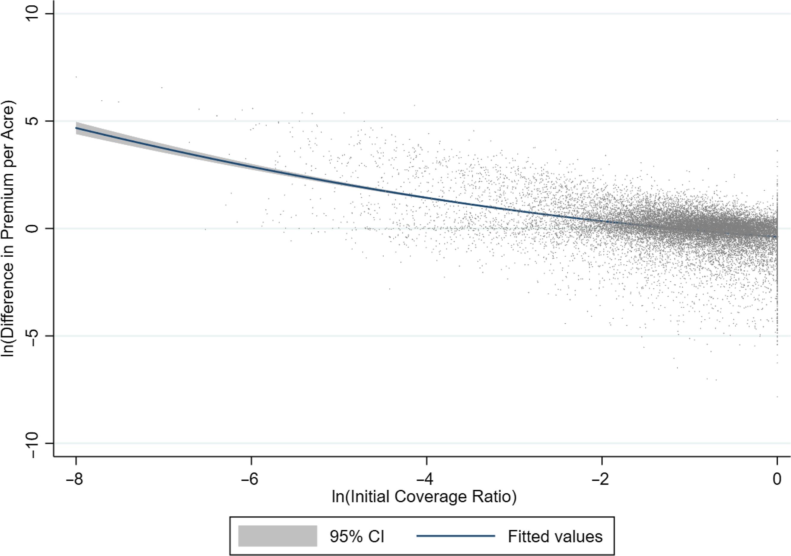
Figure 5. Relationship between logarithm of coverage ratio and logarithm of change in crop insurance premium per acre.
Results
The matching estimator estimates the causal effects of crop insurance participation on farm input use. Though preferred, this estimation relies on the selection of observables. The matching method may result in biased estimates if any unobservable affects producers’ risk-taking behavior because crop insurance participation decisions likely correlate with errors. Controlling for unobserved heterogeneity using fixed effects may result in better estimates. Thus, the robustness of estimates is determined using the matching and fixed effects approaches.
We use the covariate balancing propensity score matching estimator to identify crop insurance enrollment effects on farm input use. Figure 6 shows the univariate balance for each covariate before and after matching using the love plot (Greifer, Reference Greifer2018). The love plot summarizes differences in the observed covariates between insured farms and their matched controls. Since the absolute mean difference is within the threshold of 0.1 (dashed line), the love plot in Figure 6 shows that balance is achieved for the covariates in the matched (adjusted) sample. The balance of distributions (density plots for continuous variables and bar charts for binary variables) assessed using bal plot Footnote 8 (Greifer, Reference Greifer2018) shows a good overlap for all the covariates between treated and control groups after conditioning. Achieving a good overlap is essential to infer that the only difference in input use between insured and uninsured farms occurs due to crop insurance participation.
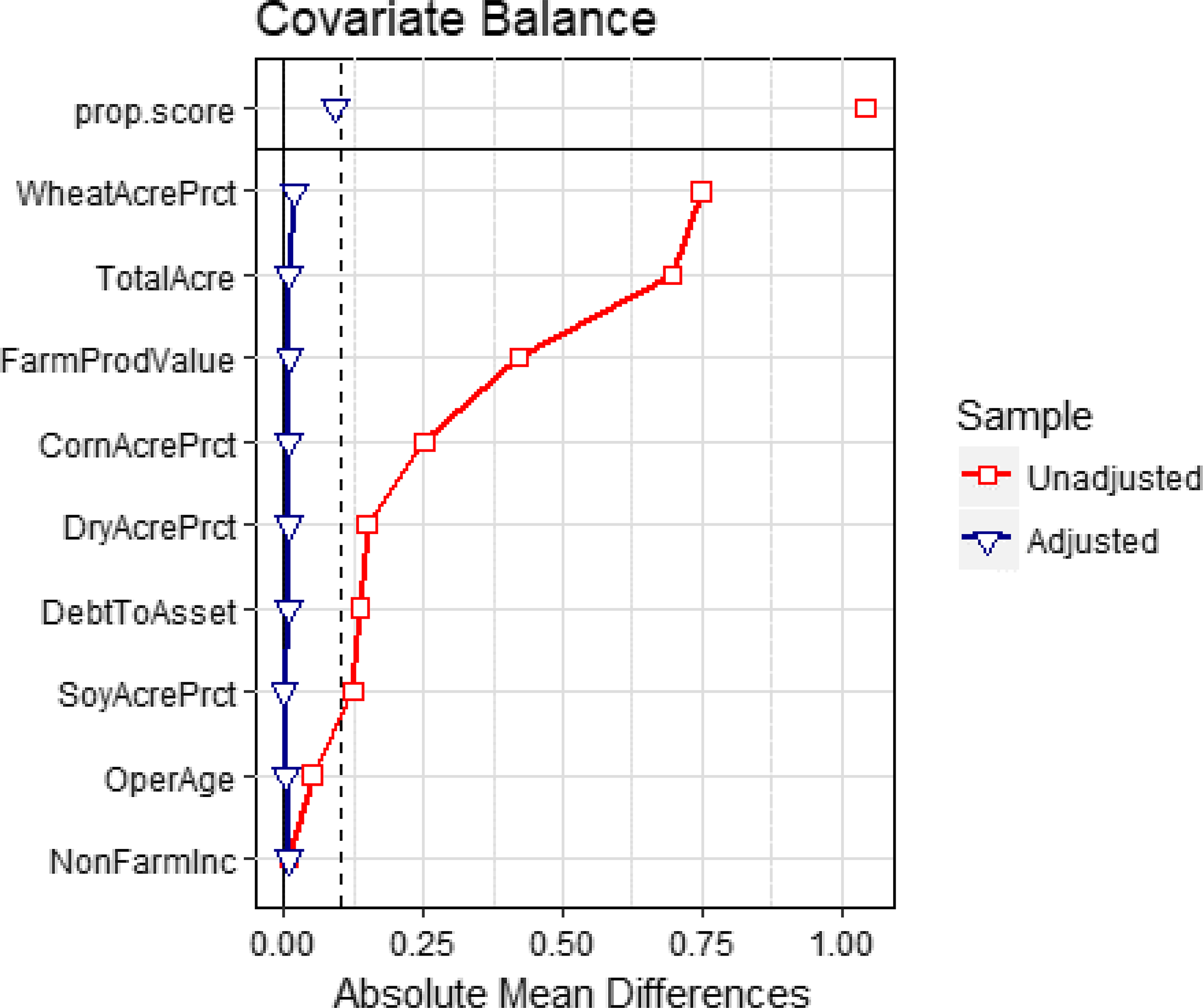
Figure 6. Covariate balance for propensity score.
Table 3 presents the average treatment effect on the treated (farms with crop insurance) for CBPS matched sample. Insured farms spend an additional $2.18 per acre on fertilizer, $2.22 per acre on agrochemicals, and $1.47 per acre on seed than uninsured farms. Each of these estimates is significant at the one percent level of statistical significance. The average treatment effect estimates suggest that an average size farm in Kansas (with 1,039 crop acres based on our sample) would reduce the purchase of farm inputs (fertilizer, pesticides, herbicides, and seed) by $6,099 in the absence of crop insurance.
Table 3. Average treatment effects of crop insurance on farm input use by insured farms
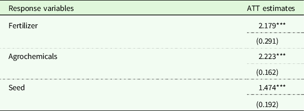
Notes: The “ATT Estimates” are obtained using Covariate Balancing Propensity Score Matching. The term “fertilizer” represents fertilizer and lime expenditures per acre, “agrochemicals” represents herbicides and insecticides expenditures per acre, and “seed” represents “seed and other crop” expenditures per acre. Standard errors are in the parentheses. ***, **, and *, respectively, denotes statistical significance at 1%,5%, and 10% level.
The results obtained using the fixed (within) effects estimator with farm and year fixed effects are presented in Columns (1)-(3) of Table 4. Figure 7 displays the results associated with the key parameter of interest (crop insurance measure). Results suggest that insured farms spend $0.97 per acre more on fertilizer, $0.65 per acre more on agrochemicals, and $0.35 more on seed (Table 4). These estimates confirm that the directional effects of crop insurance participation measures estimated using the matching estimator are robust.
Table 4. Effects of crop insurance on farm input use
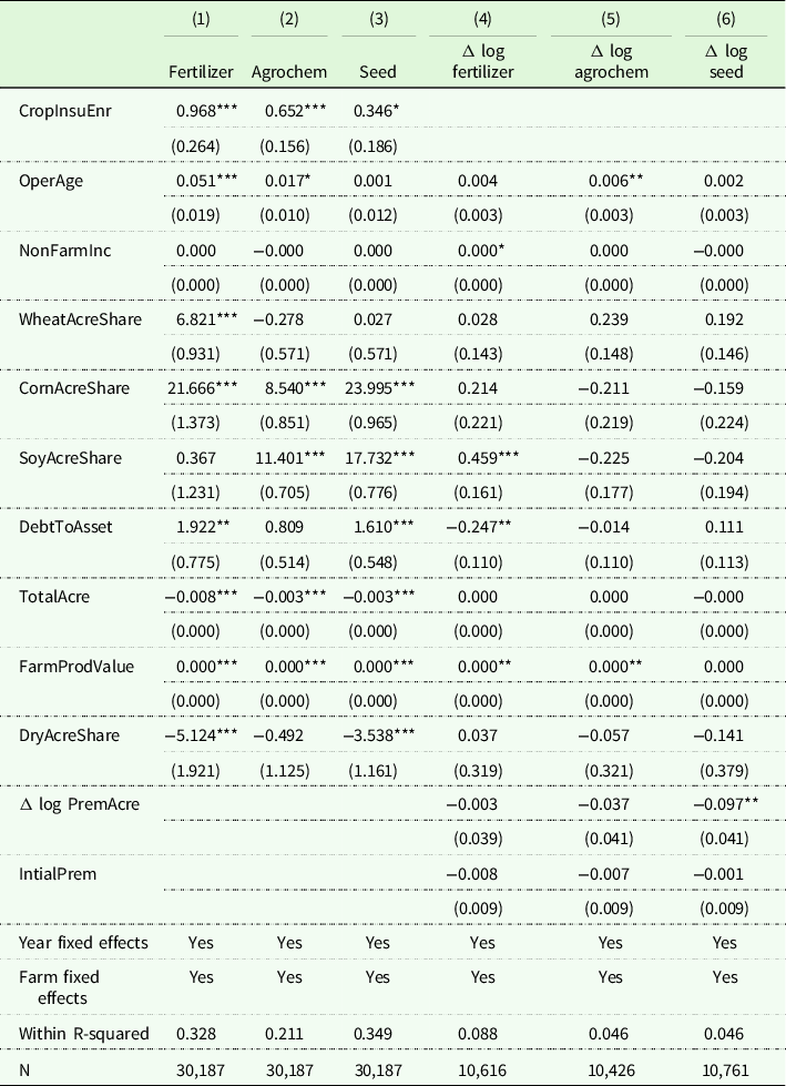
Notes: Columns (1)–(3) show the effects of crop insurance enrollment on farm input expenditures per acre after fixed effects estimations. The dependent variable “fertilizer” represents fertilizer and lime expenditures per acre, “agrochemicals” represents herbicides and insecticides expenditures per acre, and “seed” represents “seed and other crop” expenditures per acre. Columns (4)–(6) show the fixed effect instrumental variable estimation results of change in logarithm of premium per acre (crop insurance coverage) impact on change in logarithm of farm input expenditures per acre. All columns include farm characteristics such as operators age, non-farm income, wheat acre share, corn acre share, soybean acre share, debt-to-asset ratio, total acre, farm production value, dry acre share. Further, columns (4)–(6) include initial premium per acre and crop insurance coverage measure is instrumented by coverage ratio. Robust standard errors in the parentheses are clustered at farms level. ***, **, and *, respectively, denotes statistical significance at 1%, 5%, and 10% level.
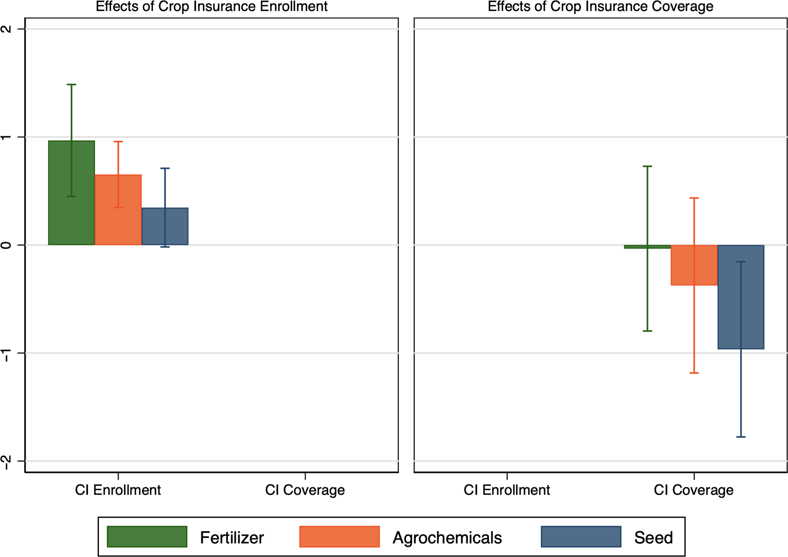
Figure 7. Marginal effects (the y-axis) of crop insurance enrollment (in the left) and crop insurance coverage (in the right) on farm input expenditures per acre.
Notes: The term “fertilizer” represents fertilizer and lime expenditures per acre, “agrochemicals” represents herbicides and insecticides expenditures per acre, and “seed” represents “seed and other crop” expenditures per acre. 95% confidence bars are shown using standard errors clustered by farms.
Similarly, Table 4 shows that a 10% increase in the wheat acre share increases fertilizer expenditures by $0.68 per acre. An additional 10% of the share of corn acres leads to a per acre increase in fertilizer by $2.17, agrochemicals by $0.85, and seed by $2.40. A 10% increase in the share of soybean acres increases agrochemicals expenditures by $1.14 per acre, and seed expenditures by $1.77 per acre. An increase in the debt-to-asset ratio by 10% increases the expenditures on fertilizer by $0.19 per acre and seed by $0.16 per acre. In contrast, an additional 100 crop acres leads to a decrease in per acre expenditures of fertilizer by $0.80, agrochemicals by $0.30, and seed by $0.30. Higher farm production value is associated with higher fertilizer and agrochemical, and seed expenditures. Results suggest that a 10% increase in non-irrigated acres leads to a decrease in fertilizer expenses by $0.51 per acre and seed by $0.35 per acre.
Both approaches identify the effects of crop insurance enrollment on farm input use. The fixed effects approach examines the impacts of change in crop insurance coverage (a continuous variable). Farm fixed effects control for any farm-level unobserved heterogeneity. However, it does not capture the effects of changes in policy or shocks in the ag-economy over time. We use the year fixed effects to capture any time-invariant factors affecting farm production decisions.
Results associated with the effects of crop insurance coverage (with endogeneity adjustment) on farm input use are presented in Columns (4)–(6) of Table 4, and in Figure 7. Unlike the effects from crop insurance enrollment, there is no statistically significant effect of an increase in crop insurance coverage on farm chemical (fertilizer and agrochemicals) expenditures. Results suggest that a 10% increase in coverage (change in premium per acre) leads to a decrease in seed expense per acre by 9.7%. Results show that a higher non-farm income, a higher share of soybean acres, a lower debt-to-asset ratio, and higher farm production value are associated with higher fertilizer expenditures per acre. Similarly, older operators and farms with higher farm production value apply more agrochemicals per acre.
A key finding suggests that crop insurance enrollment increases fertilizer applications. This implies that crop insurance enrollment is associated with higher moral hazard incentives on farm chemical use. Assuming fertilizer is a risk-increasing input, this would suggest that an average producer is near risk-neutral. Our findings also suggest that as the degree of risk aversion increases (meaning purchasing higher coverage), we do not see similar moral hazard incentives. We find that a higher coverage level is associated with a reduction in fertilizer application; though statistically insignificant, the negative sign indicates that producers may tend to apply less than optimal inputs as risk aversion increases. Our theory expected that as the risk aversion increases (meaning purchasing higher coverage), the optimal rate of input use decreases, making the second term of equation (9) (percent change in the probability that an indemnity is paid due to one unit increase in input) more negative than less negative (Babcock and Hennessy, Reference Babcock and Hennessy1996). This result is consistent with the general finding of Babcock and Hennessy (Reference Babcock and Hennessy1996): fertilizer rate decreases as the coverage level increases.
Conclusions
Crop insurance is an important safety net for insured farms during low crop revenue years. The federally subsidized crop insurance program in the U.S. may incentivize changes in farm production decisions. The moral hazard literature implies that insured farms may apply less risk-reducing farm inputs. In contrast, there exists empirical evidence that insured farms apply more farm chemicals, driven by the shift towards higher input-demanding crops. Most importantly, limited prior research accounts for the heterogeneity in moral hazard and its implication for input use at the farm level.
This research examines the effects of crop insurance on farm production practices using Kansas farm-level data from 1993 to 2016. We use matching and fixed effects estimators to obtain estimates of crop insurance participation on farm input uses. The fixed effect estimator allows heterogeneity in moral hazard among producers. We use the fixed effect instrumental variable estimator to identify the impact of a change in the insurance coverage on farm input uses.
We find that insured farms spend more on farm chemicals and seed per acre than uninsured farms. Enrollment in the federally subsidized crop insurance program leads to an increase in farm input use. This study estimates that an average size farm in Kansas spends $6,099 less in farm inputs (fertilizer, pesticides, herbicides, and seed) in the absence of crop insurance.
We do not find a statistically significant effect on farm chemical (fertilizer and agrochemical) use per acre due to changes in the level of crop insurance coverage. This finding is broadly consistent with the theoretical arguments of Mieno, Walters, and Fulginiti (Reference Mieno, Walters and Fulginiti2018) who find a lower degree of moral hazard in a dynamic input use model, and almost no moral hazard associated with low coverage rates. Based on observations over twenty-four years, the decrease in moral hazard in input use could be due to an improvement in understanding of crop conditions as argued by Yu and Hendricks (Reference Yu and Hendricks2019).
Farms that enroll at higher coverage levels do not necessarily have different behavioral responses regarding input use. This finding is of interest to policy-makers as it implies that encouraging farmers to buy higher crop insurance coverage levels through an increase in premium subsidy may not lead to a higher moral hazard in farm chemical applications. In addition, the results should be of interest to agricultural input retailers as a lessening of the crop insurance subsidy could lead to a reduction of crop input sales if many farms abandon the purchase of crop insurance.
The generalization of our findings to other regions is limited because we use farm-level data only from Kansas. Risk management approaches vary regionally based on production systems and risk ratings. Future research could consider regional differences in estimating the effects of crop insurance on farm input use. Another limitation is that KFMA data do not collect information on which crop is insured and how many acres of that crop are insured. As some crops are more input-demanding than others, our results based on the whole farm aggregates should be interpreted with caution. Future works could focus on disentangling the impacts of crop insurance on farm input use separately for different crops or crop mixes.
Data availability statement
We use Kansas Farm Management Association (KFMA) farm-level data.
Funding statement
This work was supported by the fellowship from Arthur Capper Cooperative Center (ACCC), Kansas State University.
Competing interests
None.


 Open access