

Introduction
Anthropogenic influences have affected both land cover and biodiversity across the planet. The Anthropocene period, in fact, is so named to reflect humans’ dominant impact on climate and the environment (Steffen, Crutzen, and McNeill Reference Steffen, Crutzen and McNeill2007, Steffen et al. Reference Steffen, Grinevald, Crutzen and McNeill2011; McGill et al. Reference McGill, Dornelas, Gotelli and Magurran2015). Human activity changes the earth's ecosystems, and changes in these ecosystems also affect human wellbeing. This research quantifies some of these feedback effects using applied welfare theory from economics to measure changes in the wellbeing of one group of recreationists—eBird members in the Pacific Northwest—resulting from the effects of climate change on both land cover and the spatial distribution of bird species. Our key concern is that forecasted changes in land cover and the ranges of bird species will not be uniform across space, and thus there will be shifts in the relative attractiveness of birding destinations across the region. Birders will re-optimize in response to changes in conditions, and there may be some winners and some losers. This paper focuses on variation across space in birders’ wellbeing, in the form of economic measures of the predicted equivalent variation in welfare levels associated with forecasted changes in birding opportunities.
Birds certainly adapt spatially to changes in conditions far more quickly than do plant species. This exceptional mobility affords a valuable opportunity to explore near- and short-term (the 2020s and 2050s) and spatially indexed variations in the species richness of bird populations. There have been discernible changes over time in bird species ranges and migration patterns (Pearce-Higgins, Green, and Green Reference Pearce-Higgins, Green and Green2014, Langham et al. Reference Langham, Schuetz, Distler, Soykan and Wilsey2015, Bateman et al. Reference Bateman, Pidgeon, Radeloff, VanDerWal, Thogmartin, Vavrus and Heglund2016, US EPA 2016). Notably, Pacifici et al. (Reference Pacifici, Visconti, Butchart, Watson, Cassola and Rondinini2017) find in their study that as many as one in five (of the 1,272 studied species) have experienced negative impacts of climate change in some portion of their ranges. Other studies have looked at changes in the ranges of bird species in specific countries and found similar shifts northward (e.g., Great Britain, see Thomas et al. (Reference Thomas and Lennon1999), Renwick et al. (Reference Renwick, Massimino, Newson, Chamberlain, Pearce-Higgins and Johnston2012)); as well movement to higher altitudes in some cases (e.g., Costa Rica, see Pounds, Fogden, and Campbell (Reference Pounds, Fogden and Campbell1999)).
Of course, anthropogenic influences on wild bird populations are numerous and not limited solely to climate change. Land-use change, including urbanization and conversion of natural areas to agriculture creates steady pressure on ecosystems that support bird populations (Millennium Ecosystem Assessment 2005). Species richness and species evenness (e.g., the Shannon index, an alternative measure of bird biodiversity) both tend to decrease towards the core of an urban area, with an increasing proportion of more-resilient non-native species being seen closer to the urban center (Blair Reference Blair1999, Marzluff Reference Marzluff2001, McKinney Reference McKinney2002, Marzluff et al. Reference Marzluff, Clucas, Oleyar and DeLap2016).Footnote 1 The bird species best able to adapt to urban areas are those that benefit from bird feeders and ornamental plants. Species composition in these areas is based to some extent on vegetation in both yards and parks, as well as the supply of food provided in bird feeders. In rural regions, land-use change can dramatically alter the availability of natural habitats for birds and other wildlife. Conversion to agriculture, for example, continues to reduce the availability of grassland and wetland habitats in the United States (Lark, Salmon, and Gibbs Reference Lark, Salmon and Gibbs2015, Morefield et al. Reference Morefield, LeDuc, Clark and Iovanna2016). Climate change also has the potential to affect land cover over time as conditions change (Sohl et al. Reference Sohl, Sayler, Bouchard, Reker, Friesz, Bennett, Sleeter, Sleeter, Wilson and Soulard2014).
Changes in the spatial distribution of birding opportunities across the region are of interest for their welfare effects on birders themselves, and we acknowledge that the relative attractiveness of different birding destinations is relevant when it comes to the economic impact of birding activity for nearby communities. Many towns in the region have learned that birding-related tourism, or avitourism, represents a non-trivial potential source of revenue for providers of food and lodging and suppliers of birding-related materials and equipment. Our paper focuses on the use of birding-related data for welfare assessment, but we acknowledge the potential for similar data sources to inform economic impact assessments to complement data-gathering efforts such as the birding addendum to the National Survey of Fishing, Hunting, and Wildlife-Associated Recreation (Carver Reference Carver2013).
The Literature Review section briefly describes the relevant earlier research. The Data section outlines the various datasets employed in our analysis. The Methods section sketches our approach, including our enhanced random utility maximization (RUM) model, its estimation, and our approach to the forecasting exercises in this paper, including how we calculate the expected per-trip welfare changes for birders based on our estimated model. The Estimation section briefly discusses our parameter estimates and our choice of a preferred specification. The Welfare Calculations section discusses our estimated welfare effects for these birders for a specific business-as-usual (A2 scenario) climate change scenario for the 2020s and 2050s. Lastly, we offer some conclusions and directions for future research.
Literature Review
The various impacts of climate change on several outdoor recreational activities other than birding have been considered. For example, Wall (Reference Wall1998) argues that the demand for some recreational activities is often greater when the weather is comfortably warm and dry. However, climate change may reduce some types of recreational opportunities. A lack of snow, for example, will limit snow sports. Loss of habitat for fish or game will limit fishing and hunting. Richardson and Loomis (Reference Richardson and Loomis2004) look at how visitation to the Rocky Mountain National Park would change and find that weather-related and resource-related variables that are considered in future climate scenarios are statistically significant determinants of respondents’ contingent visitation behavior. Shaw and Loomis (Reference Shaw and Loomis2008) infer how changes in temperature, precipitation, and climate variability may affect different types of climate-sensitive recreational activities (e.g., boating, golfing, and snow sports) and predict increased participation in warm-weather activities such as boating, golfing, and beach recreation, and decreased participation in cold weather activities such as skiing. Dundas and von Haefen (Reference Dundas and von Haefen2017) estimate the effects of climate change on shoreline fishing choices of anglers in the Atlantic and Gulf Coast regions, where they project an overall welfare gain in the Mid-Atlantic area and New England, and an overall welfare loss on the Gulf Coast.
As bird ranges shift in response to climate change, bird watchers may no longer see the same resident or migratory species that have historically been present, in different seasons, at their favorite birding sites (i.e., eBird “hotspots”).Footnote 2 These losses may reflect regional declines due to displacement, or overall declines in the worldwide populations of these birds (Lundhede et al. Reference Lundhede, Jacobsen, Hanley, Fjeldså, Rahbek, Strange and Thorsen2014). The disappearance of species may adversely affect the utility of bird watchers in that locale and may not be offset by the new species appearing in areas where they were not previously observed.Footnote 3 Both the forecasted losses and the forecasted gains in bird species may thus be relevant to our accounting of the potential costs (and/or benefits) associated with these changes.
Why might the social value of bird species richness (i.e., the number of different species present) be an issue of general interest? Bird watching is a popular recreational pursuit; roughly 20 percent of the US population considers themselves to be “bird watchers” (Carver Reference Carver2013). Thus, it is important to consider how these particular recreators may be affected, as part of a thorough accounting of all the costs and benefits of climate change. It also may be prudent for policy makers to consider the potential heterogeneous distributional effects across groups of birding enthusiasts as a result of business-as-usual policies concerning climate change and land use. In broader deliberations about climate change policies, what are the distributional and equity consequences, specifically for birders, that policy makers might wish to consider?
Our research seeks to forecast only the overall net monetized changes in per-trip birder wellbeing derived from birding excursions as a result of changes in species richness and land-cover in the Pacific Northwest region of the United States, under the A2 scenario (a business-as-usual climate scenario offered in the IPCC (2007) report). We address this research question using a random utility model (RUM) of destination choices for a sample of eBird citizen scientists in the Pacific Northwest. We extend the modeling framework developed in Kolstoe and Cameron (Reference Kolstoe and Cameron2017) to include land cover, thus making our basic model more flexible and more suitable for use to address how utility will change both directly and indirectly as a result of anticipated land-cover change.Footnote 4 How bird populations will be affected by climate change is related to land cover changes, because bird-range forecasts look specifically at climate suitability and habitat adaptability.Footnote 5 As a consequence, it is important to include similarly modeled land cover at each birding destination as an additional distinct determinant of birders’ willingness-to-pay (WTP) for a birding excursion.
Based on forecasted changes in land use and the ranges of bird species, we derive the formal utility-theoretic “equivalent variation” (EV) measure for each eBird member in the sample, assuming that (a) they consider the same lists of alternative birding destinations on each choice occasion as they did during the sample period of 2010–2012, but (b) there are changes in land cover and the spatial distributions of bird species across these destinations, due to the forecasted climate effects (specifically for the “A2” climate scenario, for the 2020s and 2050s).Footnote 6 Our analysis predicts that there will be significant spatial heterogeneity across eBirders in the estimated welfare effects, including both positive and negative changes.
This paper makes the point that the prospective distributional consequences of a business-as-usual policy with respect to climate change are important, not just the overall average welfare changes across all birders. The forecasted future patterns of bird species richness and land cover differ across the region under the business-as-usual policy. Changes to birding-destination attributes drive the welfare changes in our analysis. It is important to recognize that our models of birder destination choices do not involve any detailed individual-specific sociodemographic or political ideology variables as shifters of birders’ preferences. Choices across destinations are driven by the full travel cost to that destination and the attributes of the destinations themselves. Virtually all the heterogeneity in forecasted welfare effects (EVs) for birders under the business-as-usual climate scenario in this study arises from (a) differences in the spatial pattern of forecasted changes in bird species richness at the relevant set of birding destinations available to each eBirder in our sample and (b) differences in forecasted land cover changes at each destination.
Data
The eBird dataset is the product of a citizen science project built and maintained by the Cornell Lab of Ornithology. The main goal of the project is to gather data on bird populations on a year-round basis. The eBird dataset fills a niche for natural scientists who were previously limited to annual time series data from two seasonal assessments: the North American Breeding Bird Survey (BBS) in the summer, and the Audubon Christmas Bird Count (CBC) in the winter. The eBird dataset contains year-round information contributed by bird-watchers who are “members” of eBird who choose to participate by reporting their sightings to the citizen science project. The relevant portion of the dataset consists of members’ trip entries, their observed birding destinations, and their volunteered residential location information.Footnote 7 The eBird dataset provides information on spatially granular birding hotspots, so we are able to use this information to characterize expected conditions at each destination in a given eBirder's destination choice set.Footnote 8
The destination-choice dataset for this particular paper adds land-cover data from the 2011 National Land Cover Data (NLCD) as a supplement to the data used in Kolstoe and Cameron (Reference Kolstoe and Cameron2017). In terms of observations, this dataset includes 1,094 trips by 221 eBirders during the sample time period of 2010–2012, taken to birding hotspots within 60 minutes of estimated driving time from the eBirder's home, therefore involving a total of 155,495 alternatives sites across all of these choice occasions. About 75 percent of all trips were to sites within a 60-minute drive, and about 95 percent of all trips were to sites within 120 minutes. Unfortunately, we observe residential location information only at a single point in time—when members sign up for eBird. To minimize the risk of gross mismeasurement of travel costs because somebody has moved somewhere else in the region since they signed up for eBird, we limit the analysis to a three-year recent time window and use the more-restricted consideration set consisting of destinations within 60 minutes.Footnote 9
To conform with the U.S. Fish and Wildlife's definition of a “trip away from home,” we include only trips taken to a site at least one mile away from home (Carver Reference Carver2013). The calculated travel costs associated with a potential birding destination take into account both distances and travel times (based on the “best route” identified by HERE Maps and MapQuest).Footnote 10 Vehicle costs of travel are based on AAA's mileage fee for the respective year of the trip, multiplied by the roundtrip mileage. We count the value of travel time at roughly one-third of the average individual wage—in this case approximated using each birder's census-tract median income from the American Community Survey (ACS) converted into an hourly wage. The one-third proportion is a relatively common approximation in the literature (Fezzi, Bateman, and Ferrini Reference Fezzi, Bateman and Ferrini2014; Larson and Lew Reference Larson and Lew2014).Footnote 11
The key variable of interest in our model is the expected number of bird species, i.e., our “species richness” biodiversity measure, because we assume the primary purpose of these one-day trips is to see birds. To build this measure we use two sources of data: eBird and Birdlife International (see Ridgely et al. (Reference Ridgely, Allnutt, Brooks, McNicol, Mehlman, Young, Zook and International2011)) to capture species that are present year round, as well as migratory species that are present at a site only for some period of time during the year.Footnote 12
Table 1 provides summary statistics for the key trip variables and site attributes that represent the most important variables in our preferred models for the purposes of this analysis.Footnote 13 Other control variables we include in the model are indicators for site management regimes related to biodiversity, indicators for the expected presence of an endangered bird species (state and federal listings), an indicator for whether the site lies in an urban area, indicators for the type of ecosystem at the destination, and an “expected congestion” site attribute (which is based on the share of total eBird member visits to the site in question, in the same month of the previous year).Footnote 14
Table 1. Descriptive statistics across all alternatives, key variables, Oregon and Washington statesa

a Consideration sets based on 60 minute maximum travel time to alternative hotspots, 2010–2012 trips; statistics for other control variables used in our models have been relegated to the Appendix. Other controls include monthly indicators and an annual time trend in the marginal utility of E[S], four other land cover types, nine ecoregion indicators relative to the Puget Lowlands, a quadratic form in the congestion/ popularity of the destination, and interactions of the travel cost and expected species variables with a measure of the propensity (relative to the average) of this eBirder to be included in the estimating sample (221 total birders with home address information; 1,094 trips; 155,495 total alternatives; average 201 alternatives per birder (std. dev. 80.8 alternatives).
b Calculated using mqtime.ado written by Voorheis (Reference Voorheis2015).
c GAP status 1 or 2.
d GAP status 3.
For our forecasts of future conditions, we augment our estimating sample with projections of avian responses to climate change using the forecasted individual-species ranges from Langham et al. (Reference Langham, Schuetz, Distler, Soykan and Wilsey2015) and predicted changes in land use from Sohl et al. (Reference Sohl, Sayler, Bouchard, Reker, Friesz, Bennett, Sleeter, Sleeter, Wilson and Soulard2014).Footnote 15 The indicators for land cover are used to extend the basic model, reported in Kolstoe and Cameron (Reference Kolstoe and Cameron2017). These variables allow us to refine the spatial resolution of the model, as well as to facilitate incorporation of land cover forecasts into our calculations of the per-trip welfare effects of climate change for birders.
Datasets for Bird Population Forecasts
We calculate forecasted future data for bird species richness at individual birding hotspots across the region using individual species distributions predicted for the 2020s and 2050s, available in the form of an existing published dataset assembled by Langham et al. (Reference Langham, Schuetz, Distler, Soykan and Wilsey2015). This published dataset was generated from bioclimatic species-distribution models (i.e., climate niche models) for 588 species. Models were calibrated by relating observations from the North American Breeding Bird Survey data, as described in Sauer et al. (Reference Sauer, Link, Fallon, Pardieck and Ziolkowski2013), as well as the Christmas Bird Count data, to seventeen historical bioclimatic variables.Footnote 16 Models were constructed using a method known as “boosted regression trees” and employed to project the future spatial distributions of bird species under the “business-as-usual” (A2) emissions scenario across the United States and Canada, calculated at a 10-km resolution.Footnote 17 This is the most comprehensive suite of species-distribution models currently available for birds at a continental scale. The overlapping grids for each individual species can be summed across species for the region covered in our study using the Count Overlapping Polygons tool in ArcMap to yield maps of forecasted species richness. These maps can then be spatially merged to the birding hotspots in our eBird data.
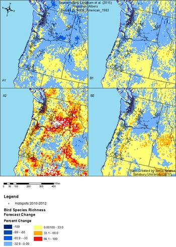
The forecasted species counts can then be used to calculate a percentage change between roughly “the present” and “the future.” The “present” data are forecasted for 2000–2009 using the species-range forecasting model, calibrated on historical data from 1980–1999. These forecasts are for 503 North American species (represented in the Christmas Bird Count data) and 475 species (represented in the Breeding Bird Survey). The two “future” time periods are roughly the 2020s and the 2050s. The calculated percentage changes in the expected number of bird species are depicted in the maps shown in Figure 1. Again, we rely on the closest available forecasts that are compatible with our framework, recognizing that if bird-range forecasts were to be updated to the most current central forecasts of future climate conditions, our welfare estimates would have to be adjusted accordingly.

Figure 1. The data from Langham et al. (2015) provides information on forecasts of bird species distributions based on the Breeding Bird Survey (BBS) and the Christmas Bird Count (CBC). The maps above show the predicted percentage change for the baseline case of 2000 to 2020 and 2000 to 2050. The forecast is based on the A2 emission scenario, a scenario consistent with business as usual
Dataset for Land Cover Forecasts
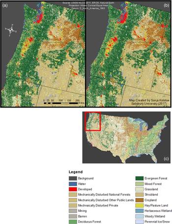
We use the 2011 National Land Cover Database (NLCD) spatial coverages (see Homer et al. (Reference Homer, Dewitz, Yang, Jin, Danielson, Xian, Coulston, Herold, Wickham and Megown2015) for more details about the NLCD) to characterize land cover at all of the different birding hotspots in the region.Footnote 18 The land cover classes included Water, Developed, Barren, Forest, Shrubland, Herbaceous, Planted/Cultivated and Wetlands, as shown in Figure 2. Relative to the Developed class, Water, Planted/Cultivated and Wetlands have statistically significantly greater value to birders, so we emphasize these particular classes in our discussion in this paper.Footnote 19

Figure 2. The forecasted land-use and land-cover for the years 2020 and 2050 under the A2 scenario. These forecasts were prepared by the USGS's LandCarbon team at the Earth Resources Observation and Science (EROS) Center for the A2 scenario using current and historical land-cover change data for the United States.
For projected future land cover, we use the forecasting scenarios of land-use change prepared by the USGS's EROS team corresponding to the same A2 scenario (see Sohl et al. Reference Sohl, Sayler, Bouchard, Reker, Friesz, Bennett, Sleeter, Sleeter, Wilson and Soulard2014) used for our bird species range forecasts.Footnote 20 A map of the current distribution of primary land cover in Oregon and Washington states is provided in Figure 2. A map of land cover overlaid with the urban area boundaries as defined by the 2010 US Census is provided in the Appendix in Figure A1 to emphasize that not all “Developed” land lies within designated urban-area boundaries, and land cover within an urban-area boundary is not always categorized as “Developed.”Footnote 21
Spatial Disaggregation of Welfare Effects
We use our estimated model to assess whether any estimated positive and negative distributional consequences for birders, as a result of a business-as-usual policy with respect to climate change and land cover, might differ systematically for different metropolitan areas and counties in the region. Recall that our model does not differentiate preferences by the sociodemographic characteristics or political ideology of the eBird members in this sample. Any heterogeneity in the estimated welfare effects thus stems primarily from the spatial patterns of expected changes in land cover and species richness. Given the spatial patterns in the forecasts for these two variables, it will be relevant to consider whether important subgroups of the population of eBirders (e.g., those living in different major urban areas in the region) might be differentially affected by the business-as-usual climate scenario we consider. Spatial variations in the distribution of welfare effects by county can also suggest how policy considerations might need to differ across regions.
Methods
RUM Model
We use a RUM model framework and assume that Ui jt is the unobserved utility derived by birder i from a trip to birding hotspot j at time t. We assume that this indirect utility consists of a systematic component, Vi jt, which can be expressed as a function of observed data and estimated parameters, and a random component that summarizes all other factors that affect utility, εi jt . This random component is assumed to be known to the birder who is making a choice among alternative hotspots in their consideration set, but to be unknown to the researcher. The systematic component of indirect utility depends on unobserved individual household income, Yi. The travel cost for birder i to reach site j is Ci jt, which is assumed to be constant over time for the data used to estimate this model.Footnote 22 The key birding hotspot site attributes in this analysis are the expected number of species available for viewing at the hotspot during the time period in question, E[S]jt, and a vector of land-cover indicator variables for that hotspot, LC jt. During the short time-frame for the trips in our estimating sample, land cover is also assumed to remain unchanged over time. We control for a vector of other site attributes for each hotspot, summarized as A jt. The simplest version of the indirect utility function, for estimation using a conditional logit algorithm, is:
 $$U_{\,jt}^i = V_{\,jt}^i + \varepsilon _{\,jt}^i = \alpha \lpar{Y^i - C_{\,jt}^i} \rpar+ \beta _0E\lsqb S\rsqb _{\,jt} + LC_{\,jt}\gamma _1 + A_{\,jt}\gamma _2 + \varepsilon _{\,jt}^i $$
However, there may be so-called network externalities among birders. In communities where birding is more popular, the marginal utility derived from richer birding experiences may be greater if an interest in birding is shared by more of one's friends and neighbors. According to Carver (Reference Carver2013), birding is a more popular pastime for higher-income individuals, so we allow the marginal utility of E[S]jt to vary with a proxy for relative neighborhood socioeconomic status, which we capture using the difference between median income in the birder's home census tract and the average of census-tract median incomes across all census tracts in Oregon and Washington states, denoted as Ydevi.Footnote 23
Bird species richness and the types of species present at a given location will vary over the seasons, as will other unmeasured site attributes and competing recreational opportunities. Thus we allow the marginal utility of expected species richness, i.e., the coefficient β0 on E[S]jt, to vary systematically with the seasons, and to shift over time, by including interaction terms for a set of monthly indicator variables and an annual time trend (a vector of variables which we denote collectively as T t).Footnote 24
Finally, due to the lack of socioeconomic data on individual eBirders that might permit us to control for other systematic variations in preferences, we choose to estimate the model using mixed logit methods (outlined below). We allow the coefficient on E[S]jt to vary randomly across individuals according to unobservable heterogeneity by including a random component, μi, in that marginal utility.
The scalar β0 parameter in equation (1) is therefore generalized to [(β0 + μi) + β1 Ydevi + β2T t]. This expression for the heterogeneous marginal utility of E[S] jt can be distributed, across the E[S]jt variable that it modifies, to reveal the key interaction terms in the estimating specification: Ydevi × E[S] jt and T t × E[S] jt, using our shorthand notation.Footnote 25
In logit-based multiple discrete choice models such as this, it is assumed that the relative indirect utility levels of the different alternatives drive the choices made by individuals. Suppose that hotspot m is designated as the numeraire alternative.Footnote 26 Relative to the numeraire, indexed by m, the utility difference associated with alternative birding hotspot j is given by:
 $$\eqalign{\lpar{U_{\,jt}^i - U_{mt}^i} \rpar= & \alpha \lpar{ - \lpar{C_{\,jt}^i \!-\! C_{mt}^i} \rpar} \rpar \!+\! \lsqb{\lpar{\beta _0 \!+\! \mu ^i} \rpar \!+\! \beta_1Ydev^i \!+\! \beta_2T_t} \rsqb\lpar E\lsqb S\rsqb _{\,jt} \!-\! E\lsqb S\rsqb _{mt}\rpar \cr & + \lpar LC_{\,jt} - LC_{mt}\rpar \gamma _1 + \lpar A_{\,jt} - A_{mt}\rpar \gamma _2 + \lpar{\varepsilon _{\,jt}^i - \varepsilon _{mt}^i} \rpar} $$
In this way, the unmeasured individual household incomes conveniently drop out of the utility differences, so no measure of absolute income is required for estimation. Ydevi, again, is not a household-specific income measure. Instead, as in Kolstoe and Cameron (2017), it is merely a proxy for “approximate neighborhood relative socioeconomic status compared to the rest of the region,” based on census-tract median household income in the eBirder's census tract relative to the average of this variable across all census tracts in the two-state area.
Mixed Logit Estimation
Mixed logit models are based on probabilities that individual i will choose alternative j on choice occasion t. If a specification involves both fixed and random parameters, as does our model in equation (2), we can partition the vector of coefficients to be estimated into two subsets. In what follows, let δ = (β0 + μi) be a random parameter and let θ = (α, β1, β2, γ1, γ2) remain fixed parameters. On any given choice occasion, then, the mixed logit choice probabilities are given by:
 $$P_{\,jt}^i = \mathop \int \nolimits L_{\,jt}^i \lpar {\rm \delta}\comma \; \theta \rpar f\lpar {\rm \delta} \rpar d{\rm \delta} $$
where Li jt(δ,θ) is the conventional logit probability evaluated at parameters (δ, θ), based on the systematic portion of the utility derived from each alternative, Vi jt:
 $$L_{\,jt}^i \lpar {\rm \delta}\comma \; {\rm \theta} \rpar = \displaystyle{{{\rm e}^{V_{\,jt}^i}} \over \sum\nolimits_k {\rm e}^{V_{kt}^i}} $$
and where f (δ) in equation (3) is the density function for the random parameter δ. The mixed logit choice probability is thus a weighted average of the logit formula computed at different values of δ, with the weights given by the density function f (δ). Tailored to our example, let f (δ) = φ (δ|β0,σ2μ), so that the mixed-logit probabilities are:
 $$P_{\,jt}^i = {\int} \left(\displaystyle{{\rm e}^{V_{\,jt}^i} \over \sum\nolimits_k {\rm e}^{V_{kt}^i}} \right) {\rm \phi} \left({\rm \delta} \vert {\rm \beta}_0, {\rm \sigma}_{\rm \mu}^2 \right)d{\rm \delta}$$
where all of the fixed parameters θ in our model, and the random δ coefficient as well, are embedded within the expressions for Vi jt inside the large parentheses.
Forecasting Per-Trip Welfare Changes Under Climate Change
Utility derived from a birding trip, in our model, is driven almost entirely by travel costs and destination attributes.Footnote 27 We wish to explore the welfare consequences of forecasted changes in the spatial distribution of expected bird species richness, along with forecasts of land cover changes across the sample region, given a business-as-usual climate forecast.
Our estimates of individual welfare change begin with the estimated utility parameters based on actual conditions, combined with the actual levels of the explanatory variables to infer the maximum attainable systematic utility level, under current conditions, across all birding destinations in the eBirder's consideration set.Footnote 28 We then retain the same set of utility parameters, but permute the levels of the key explanatory variables (i.e., species richness and land cover) according to the forecasted effects of climate change on these variables. We then infer the revised maximum attainable utility level across the same set of destinations under these new conditions. The most preferred destination under the forecasted new conditions may be the same as under the actual conditions, or it may change. We do not seek to predict exactly which site will be visited under the new conditions. We seek only to infer the maximum attainable systematic utility across all destinations under the new conditions.
We monetize the before-and-after utility difference to calculate what difference in income under unchanged conditions would leave each eBirder with the same per-trip utility from birding excursions as they would obtain with the forecasted change in conditions but no other adjustment to income. Technically this dollar amount is an equivalent variation (EV). If the forecasted EV is positive, the policy in question makes the eBirder better off; if the forecasted EV is negative, the policy makes the eBirder worse off.Footnote 29
The Algebra of Per-Trip Welfare Change Calculations
Based on our parameter values estimated in the context of utility-differences, we can revert to express the level of systematic utility, Vi jt, for individual i, associated with a trip to hotspot j in month t, as:
 $$\eqalign{V_{\,jt}^i & = \alpha \left( {Y^i - C_{\,jt}^i } \right) + \left[ {\left( {\beta _0 + \mu ^i} \right) + \beta _1Ydev^i + \beta _2T_t} \right] E\left[ S \right]_{\,jt} + LC_{\,jt}\gamma _1 + A_{\,jt}\gamma _{2\; } \cr & = \alpha (Y^i) - \alpha \left( {C_{\,jt}^i } \right) + W_{\,jt}^i } $$
where the abbreviation Wi jt merely economizes on notation in what follows.
Across all of the J i alternative hotspots in individual i’s consideration set, the “log-sum-exp” transformation, ln{Σk exp(Vi kt)}, can be used to approximate the maximum attainable systematic indirect utility from any destination in this set of alternatives. In our model, household income does not vary across alternative destinations (birding hotspots), although travel costs do. Thus, a term exp[α(Yi)] (in the following equation) can be factored out of the sum over alternatives k = 1,…, J i for eBirder i in the log-sum-exp expression.Footnote 30
 $$\eqalign{{\rm ln}\left\{{\mathop \sum \limits_{k = 1}^{J_i} \exp \lsqb{V_{kt}^i} \rsqb} \right\}&= {\rm ln}\left\{{\mathop \sum \limits_{k = 1}^{J_i} \exp \bigg[ \alpha \lpar Y^i\rpar - \alpha \lpar{C_{kt}^i} \rpar+ W_{kt}^i \bigg] } \right\}\cr& = \alpha \lpar Y^i\rpar + {\rm ln}\left\{{\mathop \sum \limits_{k = 1}^{J_i} \exp \bigg[{ - \alpha \lpar{C_{kt}^i} \rpar+ W_{kt}^i} \bigg]} \right\}} $$
Recall that the estimated coefficient on the travel cost variable in our conditional logit model gives  $ - {\hat \alpha} $ because travel cost is subtracted from the implicit income variable, Y i.
In general, one expects some difference between the compensating variation (CV) and EV measures of the utility change associated with a change in conditions. When there are no income effects, however, these alternative measures will be the same. In our model, the indirect utility function is assumed to be additively separable in (unobserved) individual household income. Travel cost is the only money-denominated site attribute. The marginal rate of substitution between each site attribute and travel costs conveys the marginal willingness to pay for each of these attributes, which is independent of the individual birder's own household income in our specification. Relative socioeconomic status for the eBirder's neighborhood, captured crudely by our Ydevi variable, is nevertheless allowed to shift this marginal willingness to pay.
We can simulate changes in any of the variables Wi kt in equation (6), to produce W*i kt . The term includes the key expected species variable, E[S]kt, and the land cover indicators, LC kt, for our climate change simulations. The per-trip equivalent variation, EVi t can be calculated using the following formulas (adapted from p. 283 of Freeman, Herriges, and Kling (Reference Freeman, Herriges and Kling2014)):
 $$\eqalign{ EV_t^i & = \displaystyle{1 \over \alpha} \left\{ {{\rm ln}\Bigg[ {\mathop \sum \limits_{k = 1}^{J_i} \exp \lsqb {V_{kt}^{{^\ast}i}} \rsqb} \Bigg] - {\rm ln}\Bigg[ {\mathop \sum \limits_{k = 1}^{J_i} \exp \lsqb {V_{kt}^i} \rsqb} \Bigg]} \right\} \cr & = \lpar {\Delta Y^i} \rpar + \displaystyle{1 \over \alpha} \Bigg\{ {\rm ln} \left\{ {\mathop \sum \limits_{k = 1}^{J_i} \exp \Bigg[ { - \alpha \lpar {C_{kt}^{{\rm {^\ast}}i}} \rpar + W_{kt}^{{\rm {^\ast}}i}} \Bigg]} \right\} \cr & - {\rm ln}\left\{ {\mathop \sum \limits_{k = 1}^{J_i} \exp \Bigg[ { - \alpha \lpar {C_{kt}^i} \rpar + W_{kt}^i} \Bigg]} \right\} \Bigg\}} $$
when preferences are linear in net income, for scenarios where there is no (predictable) change in the level of real income, it is moot whether income (i.e., the budget constraint) is measured annually, monthly, or over some other time period. Income drops out of the utility difference entirely. This accounts for the expedience of the common assumption that preferences are linear and additively separable in the net income, Yi-Ci kt, associated with each alternative.
The log-sum-exp function yields an approximation to the largest of the exponentiated terms in the sum in question. In this utility-theoretic context, this largest term corresponds to the highest attainable utility across the consideration set. This may not always be the destination actually chosen in each case, because of the random component in the utility function, but it is the destination with the largest predicted utility. In equation (8), then, the identity of the destination predicted to yield the highest utility in the estimation sample will depend on the characteristics of each destination, summarized as its corresponding Wi kt term. The identity of the destination predicted to yield the highest utility in the forecast period will depend on the forecasted characteristics for each destination, summarized by its corresponding W*i kt term. In this case, the real costs of travel are assumed to remain unchanged, so the –α(C*i kt) term remains the same. Our EV measure thus monetizes the difference in maximum attainable utility level across all destinations in the choice set, as a consequence of spatially explicit forecasts for changes in land cover and bird species distribution.
In this paper, we do not seek to predict changes in the expected numbers of trips to birding destinations in different areas. With larger samples and richer data, it should be possible also to use models such as these to help forecast which birding destinations are likely to see more visitors and which may see fewer, with implications for changes in the economic impact of birding activity on local economies. Given the limitations of the current sample, we seek only to estimate per-trip welfare effects, rather than to develop a comprehensive model for the overall numbers of trips to each destination.
Estimation Results
Recreational Site Choice
Consideration sets: We assume that the consideration set for each respondent includes the selected birding hotspot on each choice occasion plus the typically huge number of other possible hotspots within 60 minutes of travel time from the individual's home address.Footnote 31
Our models indicate that σ2μ, the estimated variance of β0 (the random coefficient on the expected species richness variable), is statistically significantly different from zero. Thus mixed logit specifications are preferred over the analogous fixed-coefficient conditional logit specifications. Selected parameter estimates are shown in Table 2, for key site attributes and controls. The full estimation results are provided in Appendix Table A2.
Table 2. Progression of models, pooled Oregon and Washington sample; Key coefficients

Standard errors in parentheses. *** p < 0.01, ** p < 0.05, * p < 0.1.
Notes: Estimates estimated via STATA mixlogit.ado. These results use 500 Halton draws for the mixed logit model simulations. Baseline coefficient represents the marginal utility for an eBirder who has the average propensity of eBird members to have given their home address information at the time of registration and is visiting a rural site that is not managed for biodiversity in the Puget Lowland in January of 2012. Models are the results for choice sets within a 60-minute drive from a member's home.
Systematic sample selection corrections: The estimated coefficients in Table 2 pertain to an eBird member with average propensity to appear in our estimating sample (i.e., one having the average propensity to have provided home address information to eBird). This inference is appropriate because we allow both the coefficient on the travel cost variable and the baseline coefficient on the expected species variable to vary systematically with the fitted propensity from a separate probit model designed to explain home address provision across all eBird members in Washington and Oregon states.Footnote 32, Footnote 33
Marginal Utilities of Travel Costs  $ (C^{\rm i}_{\rm jt}) $ and Expected Species Richness $ (E[S]_{\rm jt}) $


The four columns of results in Table 2 begin by reproducing the parameter estimates for the preferred specification from Kolstoe and Cameron (Reference Kolstoe and Cameron2017). We then provide a sequence of three increasingly general mixed-logit specifications focusing on ecoregions and the new land-cover variables. Model 2 documents what happens when we simply substitute the land-cover indicators, with their greater spatial resolution, for the original coarser set of ecoregion controls used in Model 1. Whether we control for ecosystem differences makes no real qualitative difference to the key marginal utilities of travel cost or expected species. Nevertheless, we restore the ecosystem indicators in Models 3 and 4 because some of them bear individually statistically significant coefficients.Footnote 34
In Model 3, our preferred specification, the land-cover class indicators are included simply as site attributes with “main” effects on the utility derived from a birding hotspot.Footnote 35 The complete results for this model are available in Appendix Table A2. Model 4 shows that the interaction term between the “Developed” land-cover class (the baseline category) and urban area is statistically insignificant. We explored the inclusion of this interaction term out of a concern about the breadth of the “Developed” category, and in recognition of the fact that not all developed areas lie within designated urban area boundaries (see Appendix Figure A1). Given this result, we retreat to Model 3 as a sufficiently general model for eBirder preferences.
Travel costs: Ci jt . For our willingness-to-pay calculations, the marginal utility of other consumption (i.e., the negative of the α coefficient on the travel cost variable in a linear specification) serves as the denominator, so this travel-cost coefficient is very important. The results in Table 2 demonstrate that the coefficient on the travel cost variable is strongly significantly different from zero, with the expected sign. Its magnitude is also very robust across all of our specifications. All else equal, birders are more likely to visit nearby birding hotspots.
Expected species richness: E[S]jt. We are particularly interested in the marginal utility of our species richness (biodiversity) measure, represented by the expected number of different bird species at each destination based on the previous year's data for the same site in the same month. The baseline for the marginal utility of the expected number of species consists of the mean of the random parameter, β0, but there is evidence of statistically significant unobserved heterogeneity across eBirders, because the variance in this random parameter, σ2μ, is statistically significant across all specifications in Table 2.
The single mean coefficient β0, however, also applies only when we are considering an eBirder who lives in a census tract with median income equal to the average of these median incomes across all census tracts in the region, so that Ydevi = 0. Our crude sample selection correction also shifts this marginal utility, so the baseline coefficient also applies specifically for an eBird member having an average propensity to report home address information and thus to be included in our sample. Furthermore, given the seasonal variation and trend in this marginal utility, the baseline coefficient, β0, also applies specifically for the month of January in the year 2010. January is one of the least appealing months in which to go birding in this region, so it is unsurprising that in this month, the estimated marginal utility for an additional bird species is statistically indistinguishable from zero. In June and December however, the more popular months for birding and the two seasons for which we have specific forecasts of species ranges under climate change, the baseline marginal utility for an additional expected species is statistically significantly positive, as evidenced in the set of coefficients on the eleven month-specific interaction terms reported in Appendix Table A2. The marginal utility of an additional expected species also increases with the deviation of the eBirder's census-tract income from the mean in the region. Members from more-affluent areas have a statistically significantly greater marginal utility for an additional expected species in all seasons, on average.
Land-cover classes: This is the key information that is new to the models in this paper, and along with species richness, crucial for the effects of climate change on eBirder welfare levels that we seek to forecast. Among the land-cover classes, the baseline “Developed” class can range from open space to high-intensity, as defined in the NLCD 2011. Relative to that category, the subset of land-cover classes for which marginal utility is statistically different are Water, Planted/Cultivated and Wetlands. All these land-cover types typically support greater biodiversity and are more conducive to bird watching. The land-cover types that provide the highest relative utility are Water and Wetlands, and these land-cover types are what one might expect to find in some of the region's National Wildlife Refuges, all of which are managed for bird biodiversity and may be a more aesthetically pleasing setting for a bird watching trip.Footnote 36 Based on the estimates in Table 2, relative to the “Developed” land-cover class, eBird members derive statistically significantly greater utility from trips to hotspots that are characterized as Water, Planted/Cultivated and Wetlands. Population growth, climate change and development pressures are likely to alter/diminish the quality of at least some of these types of birding hotspots.
Other site attributes: In all of the models reported in Table 2, we also control for a variety of site attributes and include indicators for the prior presence of endangered or threatened bird species, different ecological management regimes, an expected congestion/popularity measure, land-cover type, and the type of ecoregion. The coefficients on the subset of site attributes which were also included in the models in Kolstoe and Cameron (Reference Kolstoe and Cameron2017) remain statistically significant and of a similar magnitude and sign. For this reason, the estimated coefficients on many of these other attributes are relegated to Appendix Table A2.
To summarize, the coefficient on the site-level indicator for the prior presence of an endangered bird species is positive and statistically significant, suggesting that a significant marginal utility premium exists for sites where one might expect to see an endangered bird species. Also, the coefficient on the indicator for sites that are managed specifically for biodiversity (National Parks, Wilderness Areas, etc.) is statistically larger in magnitude than the coefficient on the indicator for sites less-managed for biodiversity (National Forests, etc.) where extractive activities such as logging or mining are allowed. This difference may also reflect that National Parks, Wilderness Areas, etc. tend to be iconic in some way, which may explain why there is a premium on TWTP for trips to such places, regardless of their bird populations. There is an additional premium for destinations that are managed specifically for bird biodiversity (National Wildlife Refuges). This designation often coincides with the land-cover classes that bear the largest positive and statistically significant utility premiums relative to the baseline (“Developed”) land-cover class. These estimated differences seem intuitively plausible—a trip to a more-pristine area yields higher utility than a trip to a less-pristine area, independent of the number of bird species expected to be seen.
We continue to find that our prior-year congestion/popularity measure confers diminishing marginal utility. The linear coefficient on the congestion/popularity variable is positive and the coefficient on the squared term is negative. This suggests that there may exist a threshold at which a site's popularity begins to reduce people's utility, possibly as a result of congestion. If birding is a social activity, and a destination is not too crowded, additional visitors do not seem to diminish the quality of the experience. It is possible that at low levels, a little congestion is a “good” thing.
We continue to include ecoregions, as systematic shifters of utility, to avoid omitted variable bias, the utility that an individual may derive from the type of destination (i.e., ecological factors) may be separate from the incremental utility associated with the expected number of bird species at that destination. Ecoregions will also be correlated to some extent with the distance of a hotspot from the major population centers in the region, and we do not wish to bias the key travel cost coefficient by omitting this potentially relevant determinant of utility. Given the diverse array of land-cover classes within any large ecoregion, we are not worried about extreme collinearity among these two groups of indicators. There is certainly a strong likelihood that land-cover class and ecoregion indicators will be correlated with expected numbers (and types) of species present, so it is important to allow for independent effects on utility levels for all three factors. Some birders choose their birding destinations because certain hotspots have other attractive features (e.g., scenery) besides just the number of expected bird species. In our complete set of estimation results in the Appendix, the omitted land-cover class is “Developed” and the omitted ecosystem is the Puget Lowlands in Washington State. Relative to that baseline, positive and statistically significant differences in utility are found for the ecoregions designated as the Willamette Valley, the Cascades and the Coast Range.
Welfare Calculations
Actual Conditions: TWTP and MWTP by Selected Site Attributes
Under current conditions, and for the estimated utility parameters reported for Model 3 in Table 2 (our preferred specification), we calculate the effects on total willingness to pay (TWTP) for a birding excursion of (a) the key species richness variable (shown in Table 3), (b) month-of-year/season (shown in Table 4), and (c) land-cover class at the destination (shown in Table 5). Our approach is to establish an arbitrary baseline case, and then to permute the factor in question and report the resulting effect on our willingness-to-pay measures relative to that benchmark case. The relevant baseline case is summarized in the title for each table.Footnote 37 This strategy allows us to illustrate the extent of the influence of each factor on the implied total willingness to pay (TWTP) for a birding excursion and, in the case of month-of-year/seasonal effects in Table 4 on marginal willingness to pay (MWTP) for an additional expected species at the destination. The basic results in Tables 3 and 4 are similar to those obtained for our earlier models without land-cover indicators, in the corresponding tables in Kolstoe and Cameron (Reference Kolstoe and Cameron2017).Footnote 38
Table 3. Relationship between the value of a birding trip and species richness at the destination (calculated at mean congestion level, for June 2012, unmanaged site, no endangered species reported, nonurban developed destination in the Puget Lowlands)

Note: Across 10,000 draws from the joint distribution of the parameter estimates, mean and 5th and 95th percentiles of the simulated sampling distribution for calculated WTP. Interval reflects the precision of the parameter estimates.
Table 4. Systematic seasonal variations in the value of a birding trip (calculated at mean species richness and mean congestion level, for June 2012, unmanaged site, no endangered species reported, nonurban developed destination in the Puget Lowlands)

Note: Across 10,000 draws from the joint distribution of the parameter estimates: mean and 5th and 95th percentiles of the simulated sampling distribution for WTP. Interval reflects precision of the parameter estimates. BBS, Breeding Bird Survey; CBC, Christmas Bird Count. Relative to omitted month of January, only the indicators for February June, November, and December bear statistically significant coefficients in Model 3.
a When a given draw produces a negative value for calculated TWTP, we interpret these values as zero, because it is not possible to pay a negative amount for a trip. For MWTP, however, negative marginal utilities for a particular attribute are possible, in principle, so we do not censor MWTP estimates at 0.
Table 5. Variations in the value of a birding trip by type of land cover at the destination (calculated at mean species richness and mean congestion level, for June 2012, unmanaged site, no endangered species reported, nonurban destination in the Puget Lowlands)

Note: Across 10,000 draws from the joint distribution of the parameter estimates: mean and 5th and 95th percentiles of the simulated sampling distribution for WTP. Interval reflects precision of the parameter estimates. Relative to the omitted category of Developed, only the indicators for Water, Planted/Cultivated, and Wetlands bear statistically significant coefficients in Model 3. Full set of results in Appendix in Table A5.
Table 5 provides the key estimation results that are entirely new with the specification in this paper. We use the full set of parameter estimates for land-cover classes to show the extent of variation in the implied total willingness to pay for a benchmark birding trip, based solely on differences in land-cover classes. The point estimate of TWTP is about $276 for the baseline class of land cover (“Developed,” which includes open areas as well as low-intensity, medium- intensity and high-intensity developed areas). This TWTP rises as high as $286 for sites where the land cover is Water or for sites where the land cover is Wetlands. Recall that only the utility differentials for Water, Planted/Cultivated, and Wetlands are individually statistically significant. For Water and Wetlands, the TWTP differential is estimated to be about $10 per trip. The TWTP differential for Planted/Cultivated is about half that.
Our implied total willingness to pay of $276 applies for a trip during the prime bird-watching season (in June) to a site with our baseline characteristics. This addition of the land-cover attribute makes the model more usable for conservation purposes when looking at how land-cover changes are likely to affect birders’ welfare levels. This TWTP estimate is within the range found by Zawacki, Marsinko, and Bowker (Reference Zawacki, Marsinko and Bowker2000) of $18.70–$327.50 for a more-general wildlife watching trip. Our TWTP estimate is higher than that found by Dissanayake and Ando (Reference Dissanayake and Ando2014), who report upon a stated-preference survey to assess the value of grassland restoration (where bird biodiversity and density were included as site attributes). They find a TWTP between $75–$150. However, our estimates of TWTP for a birding trip vary dramatically over the course of a year in our Pacific Northwest context, as documented in Table 4—from essentially $0 in February to $276 during the peak of the breeding season in June. Our estimate of TWTP for a birding excursion in December, the second most popular birding month in the Pacific Northwest, is only $134, which is consistent with the estimates of Dissanayake and Ando (Reference Dissanayake and Ando2014).
Forecasted Policy: Business-as-Usual Climate Change
We can use our model of birder preferences to predict what may happen to the per-trip welfare of birders in this region if conditions were to match the business-as-usual (A2 per IPCC (2007)) climate scenarios for the 2020s and 2050s. More than 1000 trips across the seasons during our sample period are used to produce our utility parameter estimates, but there are correspondingly fewer trips any given month. We use the species-range forecasts estimated for June based on the USGS Breeding Bird Survey (BBS) data, and for December based on the Audubon Christmas Bird Count (CBC).Footnote 39 No forecasts are available specifically for each month in 2020s and 2050s, unfortunately, so we must improvise as follows.
Our utility model is based upon birding excursion data from throughout the year, but our two projections of avian species richness each apply only one season. Therefore, we treat the two available percentage-change projections for each birding hotspot as different predictions applying to the entire year in each of our two future time periods (the 2020s and the 2050s). The BBS and CBC forecasts are somewhat different. We use the summer-based BBS forecast, and the winter-based CBC forecast, to put rough bounds on what may happen year-round (see Figure 1).Footnote 40 These two cases should provide a crude picture of the types of welfare changes that are possible, based on the available forecasted data for changes in the ranges of bird species and changes in land cover.Footnote 41
Relative to our estimating sample of eBirder preferences for 2010–2012 in this region, Table 6 summarizes the main results for our forecasted near-term (2020) and somewhat longer-term (2050) per-trip welfare changes (measured as equivalent variations, EV). Each set of results includes the average EV across all of the trips in the sample, the standard deviation in these EVs, as well as the minimum and maximum predicted EVs. Notably, each range includes both positive and negative values, implying that there will be both winners and losers among the eBird members in our sample, with changes in land cover and the ranges of bird species and thus in species richness at different hotspots.
Table 6. Distribution across our sample of birding trips, for per-trip equivalent variation calculated from parameter point estimates only; simulated for spatially differentiated forecasted changes in region-wide land cover and bird species richness. KEY: Across our sample of trips: average per-trip EV (std. dev. in per-trip EV), [minimum per-trip EV, maximum per-trip EV]

Notes: Forecasts (1) and (2) assume the same predictions about land cover, but differ according to whether the Breeding Bird Survey (BBS) or the Christmas Bird Count (CBC) is used as the basis for predicted changes in bird species richness in the 2020s and 2050s.
The two columns in Table 6 summarize the distributions of welfare changes, across the trips in our estimating sample, for 2020 and 2050. Within horizontal Panel A of this table, and in each of the two sub-sections of horizontal Panel B, forecasted EVs are provided for separate species richness projections based first on the data from the Breeding Bird Surveys (BBS) conducted in the May–June period, and then on the data from the Christmas Bird Counts (CBC) conducted in the December–early January period. Again, we scale the entire year's species richness forecast according to these two benchmarks, to give a sense of the differences.
Panel A in Table 6 summarizes the welfare effects for the entire sample of eBirders, across all of their birding excursions. The key take-away point is that there is a lot of heterogeneity in the welfare changes across the sample. This heterogeneity stems solely from the forecasted changes in species richness and land cover across the birding hotspots in each person's consideration set. Given that almost every person has a different consideration set, the eBirders in our sample will be affected differently by climate change. For example, consider the results based on the CBC forecast for 2050. At one extreme, climate change is forecasted to result in a loss of per-trip welfare, for some eBirder in our sample, on the order of $109 (based on the BBS forecast for 2050). At the other extreme, climate change is forecasted to result in a gain in welfare, for some (different) eBirder in our sample, on the order of $106. Again, these forecasts assume the same people take trips at the same time of year and choose from the same consideration sets—but when they re-optimize under new conditions, they do not necessarily choose the same destination from that consideration set. If we forced people to continue to go to the same destination under different conditions, their maximum attainable welfare would be lower than if they can re-optimize.
Panel B in Table 6 disaggregates, subsetting the data to show the corresponding distributions for just the Seattle metropolitan area and for just the Portland/Vancouver metropolitan area (excluding the rural areas of the two states). There is no striking difference in the average welfare derived from birding excursions in these two metropolitan areas, and there remains considerable heterogeneity within each metropolitan area (see Figures A2–A5 in the Appendix).
Table 6 reveals that to look only at the means of our EV estimates across these coarse partitions would ignore some potentially important finer-scale distributional consequences. Again, the extent to which individual eBirders are affected by the forecasted changes in land cover and bird species richness depends on how conditions change at those sites included in each individual eBirder's consideration set of birding hotspots. Consideration sets vary with the residential location of the birder in question. On average across all eBirders in our sample, the point estimates of EV per trip are relatively small. However, given that the range in EV estimates is sometimes very large, it may be important to think about finer spatial resolution in the patterns of welfare effects from changes in land cover and bird species richness across different areas in the Pacific Northwest.
County-Level Spatial Patterns in Forecasted Welfare Effects
The so-called “efficiency” criterion that underlies benefit-cost analysis in economics does not automatically take into account the often equally important “equity” consequences of proposed policies.Footnote 42 In recent years, especially in the context of environmental policy assessment, researchers have been increasingly sensitive to the potential distributional consequences of proposed policies. These distributional consequences are at the foundation of the issue of “environmental justice” or “environmental equity” from the perspective of economics.
The models of eBirder preferences that we estimate in this paper involve very limited heterogeneity according to the identity of the individual birder. The closest thing we have to the sociodemographic characteristics of individual birders is the median household income for the census tract in which the birder resides, relative to the mean of these median incomes across all census tracts in this two-state area. Beyond this heterogeneity stemming from likely relative socioeconomic status, preferences are implicitly averaged across all birders in the estimating sample and do not differ by gender, age, or ethnicity (some sociodemographic characteristics along which environmental justice assessments are sometimes considered). The main way in which the policies we consider lead to differences in the EV associated with any given policy is via the location of the birder's place of residence relative to shifting spatial patterns in the populations of birds and in land cover within about an hour's drive from the person's home.
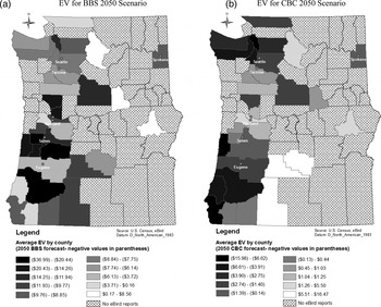
Our final exercise is to disaggregate our forecasted welfare changes for eBirders by county, across this two-state region. In the two panels of Figure 3, we depict spatial patterns in the EV associated with business-as-usual with respect to climate change in the 2050s, with the associated changes in land use and bird populations for both June (based on the BBS data forecasts) and December (based on the CBC data forecasts). To emphasize relative welfare changes, the dark-to-light shading (for counties for which our eBird sample includes data) reflects only the deciles of the distribution of EV forecasts under the BBS and the CBC forecasts for species ranges. Negative values are denoted in parentheses, and we do not force the same scale across the two maps.

Figure 3. By policy: Deciles of the distribution of county average per-trip equivalent variation (darker = more negative). (a) EV for BBS 2050 Scenario (b) EV for CBC 2050 Scenario
The fundamental take-home point concerns the unequal spatial distribution of the losses (or gains) in per-trip welfare for eBirders as a consequence of the changes in land cover and bird ranges predicted to result under the A2 business-as-usual climate forecast. Each of these two maps, independently, confirms that the consequences of climate change for birder welfare are different across counties. Given how parsimonious are our specifications, the results in Figure 3 should be taken as confirmation that even with essentially identical preferences, there can be differences in the welfare effects from policies simply because of differences in the spatial distribution of birding destination options relative to where people live and differences in the way that climate change is expected to affect bird populations and land cover across these different sets of destinations.
Caveats
Our estimates for per-trip equivalent variations for birding excursions under climate change completely ignore any “non-use” or “passive use” values derived from land cover and bird populations (e.g., existence, option, or bequest values) that might be associated with a business-as-usual climate policy. Also, the utility derived from backyard birding is likely to be sizeable. Backyard birding is not being considered at all in this study, and birders may substitute away from birding excursions and toward back-yard birding (or vice-versa) as the spatial distribution of bird species richness changes. Significant changes in local bird populations can likewise be expected to result in welfare changes from backyard birding as well as from away-from-home birding excursions, so it may be unwise to think about only the per-trip welfare effects for birding excursions away from home.Footnote 43 As with most types of economic forecasts, some maintained hypotheses underlie our calculations of the welfare effects discussed in this paper:
• All other factors affecting birding preferences and destination choices remain unchanged;
• The consideration sets of eBirders, basically a radius based on travel time from their place of residence, will be unaffected by changes in land cover or climate;
• The same types of eBirders (e.g., avidity levels) will continue to live at roughly the same residential locations, despite changes in land cover and climate;
• Each eBirder's number of trips per year will not change substantially in response to changes in land cover, climate and bird populations, although their most-preferred destinations in their choice sets may change;
• Any attempt to scale per-birder average per-trip EV estimates to the entire population of birders must be tempered by recognition that eBirders are likely a non-random subset of all birders in the region and may be more avid than the average member of the general population. Furthermore, not everyone is a birder, and some subset of the population may be completely unaffected by changes in land use and bird populations.
Climate-change-related effects on bird ranges are already being observed. However, our research suggests that changes in land cover also have an additional important direct effect for the utility that people derive from birding excursions, independent of its effects on bird occurrence. It would be difficult to tease out the overall effect of land cover on birder utility given that this factor is also bound up with its influence on future bird populations.
The results of our welfare analyses suggest that, across our sample of eBirders in different locations throughout the Pacific Northwest, there will be winners and losers as the ranges of different bird species in this region continue to shift northward or to higher elevations. These results also assume, in our bare-bones specification, that eBirders value each bird species identically. This may not be the case, but richer data and larger samples will be required to permit us to discriminate reliably between preferences across different types of species. Also, the results of Lundhede et al. (Reference Lundhede, Jacobsen, Hanley, Fjeldså, Rahbek, Strange and Thorsen2014) suggest the negative welfare effects from the loss of a familiar bird species may not be offset exactly by the gain of a new bird species, and the potential for “loss aversion” is not captured by our specifications based mostly on a simple biodiversity measure such as species richness.
Conclusions and Directions for Further Research
In the Pacific Northwest U.S., many local economies have seen a dramatic decline in extractive industries such as commercial forestry. These communities have actively sought ways to replace this declining industry, and several have learned that they have a comparative advantage in birding-related tourism. The geographic locations of these communities lie along the main flyway for numerous species of migrating wild birds, so that seasonal events such as birding festivals can be designed to draw new types of visitors who will add to the demand for food and lodging and birding-related goods and services.Footnote 44
As climate change and land-cover changes affect bird populations, though, there will be changes in the types of birds that will be available for viewing during these festivals. Our endeavor, in this work, is to provide a somewhat better picture of the benefit currently enjoyed by birders, derived from species richness among wild bird populations across the region and in different seasons. These benefits dictate the demand for opportunities to view wild birds and have the potential to affect the economic impact from birding-related tourism in the area.
The main contribution of this paper is to illustrate how citizen science data from eBird can be used to compare the potential welfare effects, for birders who travel to see wild birds, of the forecasted effects of climate and development on land cover and bird populations. Maintaining the status quo at zero cost, unfortunately, is not an option. The illustrative forecasts in this paper reveal that business as usual with respect to land cover and climate is likely to have spatially heterogeneous welfare effects. The existing literature, which provides a limited number of examples of values for specific birding sites and iconic bird species under current conditions, offers little assessment of potential future welfare impacts to be expected from land-cover change or climate change in this domain.Footnote 45
The data on birding trips used for this analysis are somewhat limited, and represent only a sample of convenience with very little information on the eBirders themselves, other than the origin point for their reported birding trips. It would be helpful to differentiate birder preferences by gender, age, ethnicity and household income levels, for example. Despite its minimal birder characteristics, the analysis demonstrated in this paper provides useful insights about the types of future studies that could potentially be conducted. With a larger data set, over a wider region (with more birding trips by more eBird members), it would be valuable to explore whether the welfare effects of a wider variety of conservation policies might vary, not just on the fine spatial scale identified in this paper, but also by type of bird, rather than just uniformly over all species. It may be appropriate, with richer data, to refine the approach in this paper also to allow for variation in the marginal utility of species richness by type of bird and/or by another biodiversity index that take species abundance into account (such as a Shannon or Simpson index).
It will also be important to develop a method to consider the representativeness of the eBird sample, both with respect to the entire population of birders, and with respect to the population as a whole. For policies that might increase utility from birding activities, it would be helpful to develop a method of modeling the number of birding trips per person, and the number of people who choose to engage in birding activities at all. Birding trip data constitute what economists call “revealed preference” data, where people are observed to incur real costs to gain access to an environmental good. But we suspect that bird populations are also valued highly by a lot of people who do not take trips away from home specifically to see birds. Backyard birding is popular, but backyard birding is more difficult to model, because no travel behavior is observed and the researcher must be more resourceful in gathering data about tradeoffs that people are willing to make with respect to local bird populations. We are currently developing in a separate “stated preference” study that seeks to measure the value of bird biodiversity among people who do not travel away from home specifically to see birds.
Managers of citizen science projects may appreciate that the data they collect to monitor bird populations can be used to model the benefits to humans derived from these populations, but this can be done well only if sufficient information is collected about each citizen scientist. Citizen science projects typically focus primarily on the behavior of the species being observed. Environmental economists are interested, instead, in the behavior of the species (i.e., homo sapiens) that is doing the observing.
Supplementary material
The supplementary material for this article can be found at https://doi.org/10.1017/age.2018.9


 Open access