


Abbreviations
- AI
-
artificial intelligence
- AM
-
area averaging of the data
- ANSYN
-
model-based performance analysis, also known as analysis by synthesis
- APD
-
alternate passage divergence
- B2P
-
blade to parameters
- BC
-
boundary condition (used in the CFD simulations)
- BDF
-
blade-definition file (RR internal file format)
- BOGV
-
by-pass outlet guide vane (OGV)
- CF
-
Centrifugal force
- CFD/fe
-
computational fluid dynamics/finite element code
- CMM
-
coordinates measuring machine
- DELT
-
lean of the blade (i.e. delta in theta direction, cylindrical coordinates)
- ESS
-
engine sector stator blade
- HH
-
Hecks & Henne function (perturbation that adds thickness to the blade)
- INMA
-
inverse-mapping process (iterative process shown in Fig. 1)
- KCF
-
key characteristic feature (monitored in the factory)
- LE/TE
-
leading edge/trailing edge
- LP/IP/HP
-
low/intermediate/high-pressure row
- LEMO
-
leading-edge movements (recambering)
- MAM
-
mid-range approximation method
- MO
-
mixed-out averaging of the data
- MRTP
-
mass-flow rate multiplied by the square-root of the T divided by P
- NRT
-
non-dimensionalised fan speed (speed divided by square root of local temperature)
- NURBS
-
non-uniform rational B-spline
- PADRAM
-
parametric design and rapid meshing tool
- PR
-
pressure ratio
- P2S
-
point-to-surface (RR internal code that measures the distance field)
- RANS
-
Reynolds-Averaged Navier-Stoke (the equations the CFD code solves)
- SKEW
-
solid body rotation about a given centre
- SFC
-
specific fuel consumption
- SLS
-
sea level standard
- SOFT
-
smart optimisation for turbomachinery (library of advanced optimisers)
- SOPHY
-
SOFT-PADRAM-Hydra (Rolls-Royce internal optimisation system)
- SQP
-
sequential quadratic programming (gradient-based optimiser)
- STL
-
stereolithography (file format)
- TEMO
-
trailing-edge movement (recambering)
- XCEN
-
sweep of the blade (vane centroid moving in the axial i.e. “x” direction)
Symbols
- m
-
mass (kg/s)
- T
-
temperature (K)
- P
-
pressure (Pa)
- R2
-
coefficient of determination, (regression model best fit)
Subscripts
- 0
-
total condition
- 1
-
core (ESS) outlet
- 2
-
by-pass (OGV) outlet
1.0 Introduction
Modern wide-chord, hollow fan blades are designed to be light but yet strong to withstand large impacts and centrifugal forces (CF) and be flexible to deform under the gas and CF loads. This phenomenon is called “untwist”. Due to manufacturing or in-service deterioration it is possible for the “running shape” of the fan blade to be altered from their design intent. Wilson et al. [Reference Wilson, Imregun and Sayma1] studied blade-to-blade geometrical variability such as tip stagger and found that the “untwist” can be amplified by the aforementioned forces, leading to a complex travelling shock-wave behaviour of the fan blade assemblies.
The effects of geometry variations on the untwist behaviour of a modern fan blade have also been studied by Lu et al. [Reference Lu, Lad, Green, Stapelfeldt and Vahdati2]. In particular, the authors addressed an unsteady phenomenon called APD (alternate passage divergence) using a blade-to-blade stagger variation much larger than the one studied previously for the buzz-saw noise ((e.g. by McAlpine et al. [Reference McAlpine, Fisher and Tester3])). They claimed that APD can adversely affect the aerodynamic efficiency and aero-mechanical stability and, unlike other types of off-design instabilities such as flutter, it can happen close to the fan operating point (i.e. close to the peak efficiency) leading to high-cycle fatigue.
The impact of the leading-edge (LE) damage on stall margin and stall inception in a low-speed fan has recently been studied by Gunn et al. [Reference Gunn, Brandvik, Wilson and Maxwell4]. Full-annulus unsteady CFD has been performed for elliptic LE blades that had been cut-backed to form a square, blunt LE. The authors found that the blunt LEs at sub-sonic speed are more sensitive to this kind of damage compared to the supersonic flow expanding around the LE, terminating in a shockwave. However, the overall effect on the stall mechanism was observed to be negligible.
A number of researchers have also studied the impact of similar geometrical parameters to ascertain the performance deterioration of compressor blades. Goodhand and Miller [Reference Goodhand and Miller5] looked at the effect of the LE shape on the LE Mach number spike and its relationship to a local flow separation as well as laminar to turbulent transition. Zheng et al. [Reference Zheng, Teng, Fan and Qiang6] numerically studied the impact of uncertain stagger angle in the last stage of a high-pressure compressor, considering the effect of multi-passages, concluding that as the number of passages considered increases, the impact of variability reduces, hence suggesting to relax the number of blades being scrapped.
Lange et al. [Reference Lange, Voigt, Vogeler, Schrapp, Johann and Gümmer7] also used a probabilistic CFD to assess impact of manufacturing variability on a high-pressure compressor performance in a multi-passage sense. They concluded the mean variation initially increases significantly in single-passage simulations, but gradually reduces to lower values when extrapolated to the full annulus. A large number of optically measured compressor blades of different IP/HP stages were studied by Lang et al. [Reference Lange, Voigt, Vogeler, Schrapp, Johann and Gümmer8]. It was found the LE shape of all rotor rows significantly affects the overall performance at maximum efficiency, while the camber line parameters of the front stages become more important than the ones of the back stages.
Although previous studies reported here add value to the body of the knowledge on compressor geometry variability effects, the same does not automatically read across to the performance of a modern, transonic, wide-chord fan blade. Evolved over many years, based on historic experience, a set of key characteristic features (KCF) that can explain the effect of manufacturing variations on the aero-mechanical performance of a fan blade has been devised and monitored at different positions along the span to ensure good conformality. These include blade parameters such as stagger angle, blade inlet and exit angles, maximum thickness value, etc. However, in this paper it will be demonstrated that these parameters may not be adequate to fully define the variation of the fan shape and hence the engine performance on a testbed.
The main aim of this research was to conduct a thorough study of real fan blade manufacturing variations and establish their detail effects on the fan performance, including validation with the real engine test data. This paper is presented in three sections. Initially, a novel inverse mapping method is first presented that allows a relatively large number of real manufactured fan blades to be inverse-mapped, producing a 3D shape parametrically. A series of high-fidelity CFD simulation is then performed on the resultant geometry identifying new key parameters that can significantly alter performance. The second part of the paper addresses the question if these deviations measured via coordinates measuring machine (CMM) in cold conditions can be translated to a variation of the hot “running shape” and indeed correlation can be carried-out with the real engine test-data. In the third part of the paper, having identified key blade features, the fan blade shape is optimised to produce a more robust blade without incurring major cost to the current manufacturing procedure.
2.0 Methodology
2.1 Inverse mapping
There are multiple ways to produce a digital model of an optically scanned blade (GOM) or using the data from a CMM. For a turbine blade, Högner et al. [Reference Högner, Voigt, Nasuf, Voigt, Meyer, Goenaga, Berridge and Vogeler9] made use of an inverse method (B2P) to morph the parametric model of a 2D aerofoil (e.g. via camber and thickness) to fit the scan data, then used another in-house tool (parablading) to construct a 3D-NURBS shape from stacked B2P aerofoil sections; the 3D blade model was then sliced at various heights by another tool, (NX2BDF) to produce a blade_definition file (BDF) which specifies the blade geometry for the CFD meshing tool PADRAM (see Shahpar and Lapworth [Reference Shahpar and Lapworth10]). This method works well when high resolution data is available, but if a blade is damaged or data is scarce, as is the case here (via cloud of the CMM data), in order not to slow down the last stage of the fan production lines, an alternative inverse-mapping method is produced.
The proposed inverse mapping workflow is summarised in Fig. 1: the starting point is a design intent blade (cold conditions), e.g. a computer-aided design (CAD) manufacturing shape, and also a set of CMM data from a manufacturing site to be used as a target. The idea of the underlying iterative process (using the optimisation library SOFT, which will be explained later) is to morph the design intent CAD blade to match as well as possible to the cloud of CMM points provided. The morphing is done by the in-house tool PADRAM, making use of its parametric design space, note that the CFD meshing of the component are automatically generated by the same tool. Another in-house tool called P2S provides the distance measurement of every CMM data by identifying the nearest surface point of the design intent blade (CAD surface) and measuring its normal distance. The aggregate of this distance field is then fed back to the SOFT optimisation library to suggest a new perturbation field, and back to PADRAM to build a new morphed blade (CAD surface) and so on. Iterations continue till the deviation distance approaches a sum of zero, i.e. a satisfactory match is achieved. In the following sections individual constituents (codes) of this workflow are explained in more detail.
The novel inverse method has successfully been applied to the by-pass outlet guide vane (BOGV) by Shahpar [Reference Shahpar11], and more recently by Carta et al. [Reference Carta, Ghisu and Shahpar12] to a shrouded high-pressure (HP) turbine rotor to study the effect of the manufacturing and in-service deterioration, respectively. Figure 2 shows a typical distance field of a fan blade: the red contour indicates a perturbation out of the page, whilst blue is into the page, hence, the changes do not just represent a change in thickness but a modification in camber too. The green levels in the contour indicate a distance field value of nearly zero. Series of lines shown in Fig. 2(a) are the location where the CMM measurements were taken, i.e. at various constant blade heights. Figure 2(b) illustrates the outcome of the inverse mapping procedure (as described in Fig. 1), resulting in a morphed blade that almost perfectly matches the CMM data (the distance field is almost green everywhere).

Figure 1. Inverse-mapping work-flow (INMA): SOFT-PADRAM-P2S codes.

Figure 2. (a) Typical distance-field contours on the initial CMM data; (b) distance-field after the inverse mapping. Not to scale.
2.1.1. PADRAM (Parametric Design and Rapid Meshing Process)
One of the advantages of PADRAM is the automatic (templated-based) meshing for the subsequent CFD analysis of the whole low-pressure (LP) compression system. Over the last two decades, close to 1,000 templates have been created for key turbomachinery components. PADRAM makes use of a O4H multi-block structured mesh in the aerofoil (blade passages), and butterfly style meshes in the tip-gap, see Fig. 3 for details. The main mesh used has ∼4m cells in the fan passage and ∼2m in the OGV and engine sector stator blade (ESS) passage, aiming for a y+ of 1 on all viscous walls.

Figure 3 (a) PADRAM multi-block mesh for a fan blade passage; (b) butterfly tip-gap mesh, LE detail.
The number of degrees of freedom in the inverse-mapping (INMA) process is relatively large and of the order of hundreds, e.g. the PADRAM so-called engineering parameters used here is 65 (seven main categories defined at five radial stations along the span, equally spaced), whilst the number of thickness parameters is 110. Figure 4 shows some of the most used PADRAM engineering parameters in the INMA process and their signs.

Figure 4. Typical PADRAM engineering parameters used in the inverse-mapping process.
Leading-edge movement (LEMO) re-cambers the aerofoil by shearing the aerofoil sections in the circumferential direction, keeping the axial chord constant as well as the aerofoil thickness. The modification to the aerofoil shape decays quadratically towards a blending point, which could be as far back as the trailing-edge. Trailing-edge movement (TEMO) acts in an analogous way at the TE position. Solid body rotation about a given centre (SKEW) is a solid body rotation about a given axis, e.g. through LE as shown in Fig. 4. XCEN and DELT are the axial and circumferential sweeps of the section receptively; LECA and TECA are local chord adjustments at the LE and TE, respectively, again with a blending point to ensure a smooth transition to the rest of aerofoil.
The design-space parameters defined above are all applied on an unwrapped 2D section of a 3D blade in cylindrical coordinates, however, a cubic BSpline is used to stack the sections in the radial direction with five control points from the blade hub to the tip.
2.1.2. SOFT (optimisation methodology)
In order to cope with the curse of dimensionality, the INMA process (Fig. 1) is split into multiple hybrid optimisation steps, where a number of design parameters are active in that step only, then followed by a second-stage starting from the best results of the first stage and so-on. It has been found that better results are obtained if the bulk parameters like lean, sweep, skew are found first and frozen, then local parameters like the LE and TE shapes are matched with the CMM data, followed finally by a thickness matching, e.g. via bump functions (Hicks and Henne [Reference Hicks and Henne13] or H&H for short). See Table 1 for the summary of the optimisation stages, and also reference Shahpar [Reference Shahpar11] for further detail paramters involved at each phase.
SOFT offers four advanced optimisation libraries (see Shahpar [Reference Shahpar and Ginnakoglou14]). Two optimisation algorithms found to be very useful for the INMA process and used in tandem are a trust-based MAM method (Shahpar et al. [Reference Shahpar, Polynkin and Toropov15]) followed by a second-order sequential quadratic programming method. A typical convergence history of the SOFT optimisation to morph the blade using the PADRAM design space to best match the CMM data is shown in Fig. 5. It is interesting to note that almost 90% of the perturbation is captured in the first phase (i.e. engineering parameters), whilst the last phase (i.e. thickness variation via H&H) only accounts for ∼0.3% of the objective function minimisation. The normalised cost-function has dropped ∼1.0 to ∼0.1.
The significance of matching the CMM via morphing a parametric CAD (PADRAM design space) is that further work, e.g. CFD simulation, can now be carried out on these solid blades, whilst the CMM cloud of points where just a set of unstructured data sets that are hard to analyse and draw meaningful aerodynamic conclusions from. Minimising the distance field towards zero gives credibility to any conclusions made later with the parametrics that define the manufactured variations.
2.1.3. P2S (point-to-surface)
The in-house point-to-surface code makes use of a ray-tracing method to compute the shortest distance of a given point (e.g. from the CMM data) to a surface (e.g. formed by the triangulation of the PADRAM CFD surface mesh (i.e. STL format)). The prerequisite to the method to work robustly is to initially position the blade reference model adequately. This is done via the CAD design intent which is moved to a position that relates to the consistent CMM data measurements, hence avoiding using any least square fitting procedure.
Table 1. Optimisation phases


Figure 5. Typical history of the optimisation phase I (LHS) and phase IV on the (RHS).
There are different distance-field measurement algorithms available in the P2S code; however, the one used here is based on the so-called l2-norm (see Shahpar [Reference Shahpar11] for more details). The total sum of this distance field (l2-norm of all sections), e.g. as shown in Fig. 2 is then used as the objective function for the optimiser. It should be noted that l2-norm is normalised by a distance computed from the maximum and minimum values of the x, y, z coordinates of the inputted data set (i.e. the datum geometry BDF) before passing it to the optimiser. The distance-field near the LE is also curvature weighted for better accuracy.
2.2 CFD simulation
Although in this study many sets of jet engine performance data are available from the sea level state (SLS) testbed, the engine test-data is complemented by high-fidelity RANS-based simulation data. The in-house code Hydra has been validated for this kind of turbomachinery flows versus various rig experimental data over many years, e.g. see Lopez et al. [Reference Lopez, Shahpar and Ghisu16] for a similar blade. The turbulence method of choice is a helicity corrected Spalart-Allmaras (SA). Hydra is an edge-based unstructured Navier-Stokes solver, and in this study the explicit version of the code with five levels of multi-grid and Mach number pre-conditioning is used. All the simulations were carried out using steady-state single-passage method with the mixing plane between the BOGV and the ESS. It should be noted that the results were almost identical when comparing the results of the average performance of 22 fan blade simulations versus a full annulus 360o one. In the latter approach the position of each fan blade were the same as the ones used in the actual engine testbed.
2.2.1 Numerical boundary conditions
Since this investigation is focused on the actual engine test conducted at the sea level conditions, the inlet BCs are subsonic (non-reflecting) total pressure, temperature and zero-flow angle at the fan inlet for standard SLS conditions. As shown in Fig. 6, there are two exit flow BCs, one for the core engine, downstream of the engine sector stator (ESS) blade where the capacity, MRTP, i.e. $\;\dot m\sqrt {R{T_{02}}} /{P_{02}}$
is set as non-reflecting exit boundary-condition, similarly at the bypass duct behind the BOGV, the working line desired
$\;\dot m\sqrt {R{T_{02}}} /{P_{02}}$
is set as non-reflecting exit boundary-condition, similarly at the bypass duct behind the BOGV, the working line desired $\dot m\sqrt {R{T_{01}}} /{P_{01}}$
is specified (see the Nomenclature table for further definitions of parameters). To compute a full fan characteristic the bypass static pressure is altered using a non-reflecting radial equilibrium formulation and ensuring the mass flow results in the correct bypass ratio for this fan (which is 9.6). The speed of the fan corresponds to the 90%NRT and there are 22 fan blades in the full annulus set of a 3m diameter producing 84K pounds of thrust.
$\dot m\sqrt {R{T_{01}}} /{P_{01}}$
is specified (see the Nomenclature table for further definitions of parameters). To compute a full fan characteristic the bypass static pressure is altered using a non-reflecting radial equilibrium formulation and ensuring the mass flow results in the correct bypass ratio for this fan (which is 9.6). The speed of the fan corresponds to the 90%NRT and there are 22 fan blades in the full annulus set of a 3m diameter producing 84K pounds of thrust.

Figure 6. (a) Meridional computational domain – not to scale; (b) table of CFD exit BCs.
2.2.2. Thrust matching
When simulating the flow for the fan-OGV-ESS stage computation, there is a need to make sure the fan is delivering the correct expected thrust for the pseudo non-dimensional rotation speed (e.g. at 90% peak speed (NRT)). Since the computation is done at a required exit capacity downstream of the BOGV, this would translate to achieve a given by-pass pressure ratio (PR). In order to achieve this PR matching, the LP shaft speed is adjusted using a linear interpolation of the working lines at different speeds. This simulates the effect of a real engine adjusting its speed to provide the required thrust and is a fair way of assessing the relative performance of these blades. For example, the full characteristics of three blades (A, B and C) randomly chosen from relatively higher and lower SFC engines are shown in Fig. 7. During this operation, it is assumed that the core-flow of the engine does not change. It has also been observed that the relationship between the PR achieved at two slightly different speed is linear, hence the following equation can be used to compute the required rotational speed Rot t given a target PR t , using two CFD computations referred to as 1 and 2:
 \begin{align}\frac{{Ro{t_t} - Ro{t_1}}}{{P{R_t} - P{R_1}}} = \frac{{Ro{t_2} - Ro{t_1}}}{{P{R_2} - P{R_1}}}\end{align}
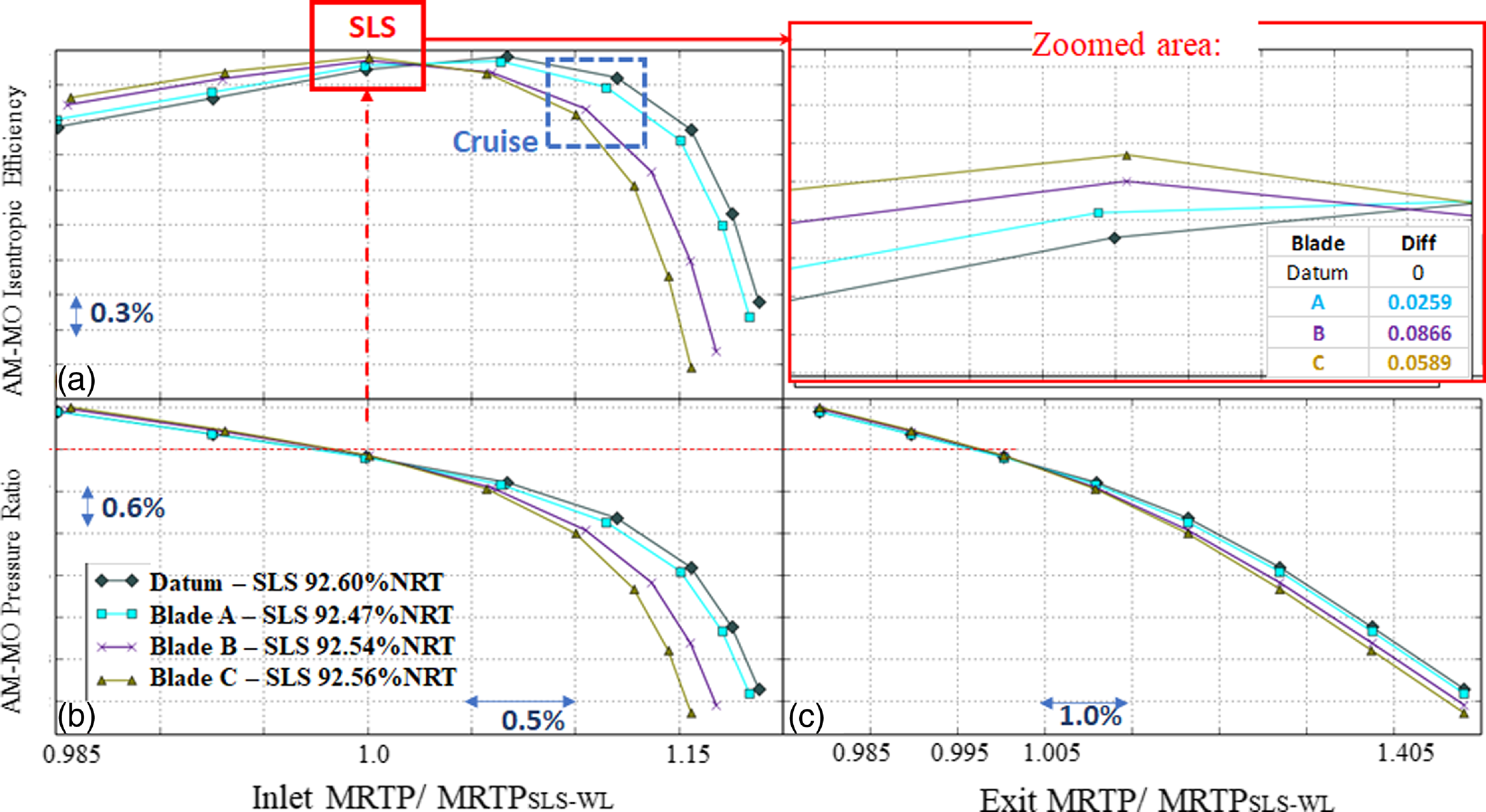
Figure 7. Fan characteristics and interpolation procedure to achieve the SLS target pressure ratio.
It can be seen in Fig. 7(b) that the fan speed is adjusted such that at given exit capacity the bypass duct is delivering the correct pressure ratio for blades A, B and C, then the fan-stage efficiency is obtained from the characteristic curve (Fig. 7(a)). MO and AM in these figures refer to the fact that primitive parameters such as pressure and temperature are mixed-out averaged (MO) in the circumferential direction and then area-averaged (AM) in the radial direction. An overall single average value of these quantities is produced before feeding them to the isentropic fan efficiency equation and also computing the pressure ratio (PR).
It is interesting to note that at this operating point, the efficiency of all three chosen blades, PR matched, is higher than the datum design intent and the delta between them is close to ∼0.1% of the fan efficiency. For the sake brevity a similar chart for cruise conditions is not shown here, but since the fan operates close to the peak efficiency (just to the right of it, towards the choke point, fifth point from the stall point in Fig. 7(a)) the change in efficiency is significantly larger of the order of 0.6–0.7% efficiency and also decreasing, i.e. opposite to the behaviour observed at the SLS conditions, third point from the left in Fig. 7(a) (highlighted in the zoomed red-box). The aerodynamic reason behind this, together with an analysis of the parameters responsible for it are discussed in the next few sections of this paper.
3.0 Results and discussions
3.1 Analysis of manufacturing variations
The manufactured blades’ CMM point cloud data is readily available as part of the standard inspection process. The novel inverse mapping process described in the methodology section of this paper is applied to 462 blades (belonging to 21 engines) manufactured over a period of two-years. To understand which geometric parameters are responsible for the difference in blade performance, each PADRAM subset of parameters was activated individually (separately) to assess the pressure-matched efficiency delta relative to the datum, i.e. what efficiency each set of parameters gives when applied on their own. An example of this for one of the best performing blades in the population (referred to as Blade D) is given in Fig. 8, similar results were obtained for other manufactured geometries giving similar trends.

Figure 8. The influence of each geometric parameter on blade efficiency for Blade D when activated individually (at SLS).
It can be seen that LEMO is by far the most influential parameter on PR matched blade efficiency, followed by Hicks-Henne bumps and SKEW. As discussed in the previous sections, LEMO is a single parameter capturing aerofoil re-cambering in the first half of the blade chord, responsible for a change in curvature on both SS and PS sides as well as in the inlet angle. TEMO is a re-cambering of the second half of the blade chord (also changing curvature in both surfaces and exit angle) and SKEW is a solid-body rotation of blade sections. All these parameters modify the blade stagger angle but could also be cancelling each other’s effects (i.e. on stagger a derived parameter). It is interesting to note that the sum of the contribution of each parameter does not quite match the overall efficiency delta relative to datum for this blade, suggesting that non-linear interactions take place between the various geometric parameters. As seen in Figure 7, the most influential parameter i.e. LEMO (drooping the LE and increasing inlet angle) raises the efficiency chic on the left of peak efficiency and reduces it on the right. It can be seen that at this operating point, the effect of LEMO on PR is minimal, so little speed adjustment is needed to maintain PR.
It is also informative to understand the effect of each parameter on the pressure ratio (measured before the PR matching step). The result is given in Fig. 9. It can be seen that TEMO has a significant impact on PR, far more than any other parameters. This makes sense as TEMO is varying the blade exit angle (−ve TEMO droops the blade TE, resulting in more turning, more work and therefore higher PR). Therefore, although TEMO has a less clear effect on efficiency than LEMO, because it can change PR significantly, it has the potential to influence the blade efficiency once PR matching (via speed) is taken into account.

Figure 9. The influence of each geometric parameter on pressure ratio for Blade D when activated individually (at SLS).
Radial plots of efficiency (not shown here due to brevity) of the aforementioned blades A, B and C reveal that the largest flow sensitives occur at around 60–95% height). This is not surprising as the relative Mach number is supersonic, and the flow contains stronger shockwaves in this region. Hence, small variations in the geometry can lead to a relatively large effect on the loss.
Looking at the shock positions at 95% span in Fig. 10, it can be seen that the better performing blades (datum to A, B and then C) have delayed shock positions (further downstream) compared to the worse performing blades (datum and A). At this SLS operating point, the more swallowed and curved the shock, the better the performance of the blade is, and the slow (blue) region of the flow (boundary-layer and the wake) is reduced. Even though a Mach spike appears near the LE on the pressure side (indicating a higher Mach number region), which is not desirable, the main bowed passage shock is more curved and hence weakened due to opening of the LE (negative LEMO).

Figure 10. Slices of the flow at 95% span for the four blades at SLS (datum shock position highlighted in a white dash line).
3.2 Engine level performance analysis
Three performance measures are available from the actual engine test-beds: these are the NL Trimmer (related to the speed at which the engine runs), specific fuel consumption (SFC) and LP-system efficiency (LPSE), which is an engine-derived parameter for system isentropic efficiency calculated by the Rolls-Royce performance office utilising an inhouse method called ANSYN. Considering the fan produces almost 70% of the engine thrust it is reasonable to assume the LP-system performance parameter from ANSYN correlates well with the KCF and/or the CFD simulation data.
In the factory there are 12 KCFs that are historically defined to monitor the conformance of the manufacturing data to the design intent. These are aggregates of the LE/TE thickness, max thickness, stagger and inlet/exit blade angles all at various heights, LE lateral and tangential lean and sweep, etc. Initially, it was attempted to correlate the aforementioned engine performance data from the SLS to KCFs, using various data analytics and an AI software. Data analytics studies in the fan factory have indicated that the blade maximum thickness is the only major parameter in the time series that shows any significant variation over time. However, the current studies indicate none of the correlations were strong. For example, as shown in Fig. 11, although different families of data are observed, the R 2 fit for the overall population versus the maximum thickness is very poor (R 2 <0.01).

Figure 11. Plot of LP-system efficiency vs. maximum thickness at 75% height.
On the other hand, it was remarkable to find that TEMO (and to a lesser extent LEMO) exhibited relatively good correlations (R 2 ∼ 0.77 and 0.4, respectively) with the engine test data, e.g. as shown in Fig. 12. There is also one outlier engine which upon careful examination afterwards had revealed an unusual cut-back on the suction-side on its TE. As explained in the previous sections, although TEMO directly does not control the fan-stage efficiency it does create a slower or faster engine which in turn translate to a more efficient fan (i.e. slower for the same thrust, as explained in the thrust-matching section). It is also worth noting that the manufacturing tolerances that control the amount of re-cambering in a blade are based on a set of tramlines and are therefore difficult to summarise as a single KCF parameter. Further analysis of R2 of other PADRAM design parameters is presented in the appendix of this paper.

Figure 12. Plot of LP-system efficiency Vs. TEMO at 75% height.
3.3 Untwist (cold-to-hot) translations
In the previous sections an assumption has been made that the difference between the cold manufactured part and the cold datum geometry (i.e. the design intent) as a set of inverse-mapped parameters can be applied to the hot running shape to produce the hot-running manufactured blade shape. This assumes that the impact of the cold blade’s manufacturing deviation from nominal on its cold-to-hot untwist is negligible. In this section, this assumption is assessed making use of a hi-fidelity in-house FE code (SC03).
A fully featured hollow wide-chord fan blade is modelled in SC03 including its root, and disk assemblies. Figure 13 shows the SC03 model and the regular brick (hex) mesh elements used in the structural analysis. The fan material is titanium, super-bonded together. Its internal hollow section boundary is shown with orange lines in this diagram. The disk section boundary conditions include cyclic constraints at either side of the disc, and zero displacement on one end and dynamic point constraints on the other. The gas loads from the CFD code (hydra) are extrapolated onto the pressure and suction sides of this blade, and engine RPM and temperature (at the SLS) conditions are also applied.

Figure 13. SC03-FE mesh used in the untwist analyses. Not in scale.
As shown in Fig. 14, for the datum blade, significant tip-stagger variation, of the order of ∼1.5o can take place under centrifugal loads (CF), whilst the gas loads (derived from a CFD run for that particular blade shape iterated to convergence) account for an additional 0.3–0.4o. The overall tip untwist stagger change is an order of magnitude larger than those observed due to the manufacturing variations. In order to assess the running-up of the cold manufactured shapes, a procedure similar to the PADRAM-P2S process of Fig. 1 was used to morph the SC03 mesh of the datum geometry to fall onto a BDF file but using the available FE mode-shapes and nodal perturbations. Once the morphing iterations are complete, the P2S is used to make sure the morphed mesh is close to the STL of the inverse-mapped surface that represents the manufactured part.

Figure 14. Variation of the tip stagger angle with the blade speed under CF and gas loads.
An example of the resulting blade shapes is given in Fig. 15 for blade “D”. It can be seen that the effect of applying the inverse mapping design parameters to the run-up datum blade gives a very similar shape to running up the manufactured cold blade. There is a slight difference with a small tangential lean away from the direction of rotation, but the overall shape is quite consistent. The P2S process indicates a limited deviation of less than 0.1mm for the two methods.

Figure 15. Comparison of the run-up blade shape using two different methods of applying perturbations.
In order to assess the robustness of the run-up process described above versus applying the cold perturbation to the hot-running shape, eight blades were chosen from the lowest efficiency to the highest efficiency across the population of 462 blades analysed. For this set, the cold reference blade is morphed into the manufactured shape and then run-up under CF and gas loads to convergence, then the same manufactured perturbation files applied to the reference hot running shape at the cruise conditions. Figure 16 shows the CFD-derived performance comparison (efficiency from the datum value) for these two sets.

Figure 16. Comparison of the efficiency variation for the eight key manufactured blades using two methods of run-up process.
Although differences occur in the predicted efficiencies, the overall ranking of the manufactured blades is remarkably similar. The efficiency difference between applying the inverse-mapped design parameters to the hot running BDF and generating the cruise manufactured BDF by running up the inverse-mapped cold blade is within 0.1% in every case. This is a significant finding for industry that simplifies future assessments of the manufactured parts negating the need to running up every blade case under manufacturing-variation investigation.

Figure 17. PADRAM parametric definition (cut-back) of the blade leading-edge.
3.4 Optimisation for performance recovery
Having understood the relationship between the engine performance and some key parameters that characterise the manufacturing variation, this section identifies ways of recovering the fan stage efficiency whilst keeping its speed under control. There are different ways to improve the fan performance, for example by tightening the manufacturing tolerances, or even using the LEMO-TEMO maps from this study to bias the average blades to another, better performing sector. However, there are 80 steps in the process of producing the Rolls-Royce hollow-wide-chord fan blade, and the aforementioned methods would inevitably lead to increase in cost of production and/or slowing down the factory yield or both. Hence, a novel way is pioneered in this study where an asymmetric LE and TE are proposed, Shahpar [Reference Shahpar17], to counteract any existing, final manufacturing variation and recover the fan efficiency.

Figure 18. Datum and optimum shape of the blade leading-edge. Not-to-scale.

Figure 19. Datum and optimum shape of the blade leading-edge.
The PADRAM design space has many interesting features: Fig. 17 shows the so-called cut-back design capability meant to simulate damaged or in-service blade shapes. However, the SOPHY optimisation system (similar to the one shown in Fig. 1 but replacing P2S with Hydra) was used to produce optimum asymmetric LE and TE within the manufacturing tolerances, e.g. see Fig. 18. Note that the reference blade chosen for the optimisation in an averaged performing blade (from the manufactured variation population, blade “H”). The design space is the ratio of a/b and c/d of the spline control points that dictate how sharp or blunt the upper (suction side) and lower (pressure side) sections can become. The edge of the resultant cubic-spline blends back to the aerofoil ensuring C2 continuity.
It is interesting to note that optimiser has increased the bluntness of the upper section, whilst reducing the thickness in the lower section almost producing a flat profile there. Although not shown here, PADRAM can also introduce a small fillet at this junction ensuring a smooth transition between the two profiles. It should be noted that although the majority of the aerofoil camber is the result of the two side of the blade titanium sheets blown apart in a die, the actual LE and TE are accurately machined afterwards. Hence, a thicker section is initially manufactured and then it is cut back to form the final exact desired blade shape, so it is quite possible to recover the proposed optimal shape exactly as designed (to compensate for the change in camber of the rest of the aerofoil).
Although the optimum leading edge and trailing edges are produced for a mean manufactured blade, its robustness had been tested by applying it to a range of blades across the 463 population of blades considered here. Figure 19 shows that applying the LE optimised design to the seven key manufactured blades at the cruise condition leads to an increase in the performance for all of them. The range of efficiency benefit is from ∼0.1% to ∼0.5%. The worst performing manufactured blade gains the most benefit from the LE optimised design, and the best performing the least, showing a clear trend. The rotational speed of all the blades has also consistently been reduced.
Further robustness studies of this optimum asymmetric LE indicated that even for an in-serviced blunt LE need dressing, the optimum LE can be introduced as a cut-back (as shown in Fig. 18), i.e. with a slightly reduced overall chord length but the benefit in PR matched efficiency hardly changes. Although not shown here in detail due to brevity, for an average blade (i.e. PADRAM parameters averaged for all the inversed mapped data) the LE asymmetry provides 0.28% efficiency whilst the LE+TE provides 0.35%. For more details refer to the Shahpar [Reference Shahpar17] patent detail. The most important “discovery” for industry is the fact that the ANSYN performance investigations indicated that this level of fan blade efficiency (leading to 0.21% SFC) is detectable from a flight test, hence paving the way for further verification of this design.
4.0 Conclusions
The main aim of this work has been to understand the relationship between manufacturing variation and fan-blade performance. This study leads to the following conclusions and also recommendations for further work:
-
1. A fast novel methodology is proposed that allows an inverse-map of manufactured blades to be produced for further CFD and FE simulations.
-
2. It is proved that that there is no need to conduct expensive untwist analysis for every blade inverse-mapped, but the shape perturbations can be directly applied to the hot-running shapes. In fact, the geometries resulting from this process are very similar and within 0.1% to the ones obtained by the running-up (i.e. calculating the deformations under the gas and centrifugal loads) the cold blades.
-
3. New perturbation parameters such as LEMO and TEMO capture the blade camber shape and are good representative of the blade suction-side curvature. These correlate well with the engine test data (0.4 and 0.78 R 2 values respectively), and significantly more than classical KCF data such as the blade maximum thickness or stagger (both less than R 2 of 0.1). CFD analysis also confirms that the LE/TE re-cambering play a major role in the fan blade performance, i.e. the pressure ratio and efficiency.
-
4. It is possible to re-dress manufactured blade LE and TE to compensate for any changes in the blade overall camber. This is a significant finding for the aero-engine manufactures, meaning that it is possible to improve the cruise efficiency of the manufactured blades by retrofitting without the expense of tightening manufacturing tolerances.
Even though, the RANS CFD code used here has been extensively validated against rig test data, it is recommended that further unsteady (URANS) simulations are conducted to further verify this paper’s key research findings.
Acknowledgements
The author would like to thank Rolls-Royce plc. for its support and permission to publish this work. The author would also like to thank Dr Alistair John of Sheffield University for contributions towards the untwist analysis and design optimisation of the fan presented here and Dr Matt Harris of CFD methods for the P2S support.
Appendix A. Further analysis of the PADRAM parameters
In this section, the result of a regression model is presented whereby the inverse-mapped PADRAM design space is linked to the engine performance data, i.e. the LP system efficiency from the Rolls-Royce performance office. In order to test the accuracy of the fitting model, a leave one out, R 2 model is carried out whereby the model is fitted recursively “leaving one data out” one at a time and computing its predicted value versus real value. Figure A.1 shows the results of this study, confirming that TEMO followed by LEMO are the main parameters affecting LP system performance with the R 2 value, 0.7–0.4 respectively, whilst SKEW, Lean and Sweep have small contributions. An attempt is also made to compute the cross derivatives, such as LEMO*SKEW, DELT*TEMO, etc. These parameters by themselves do not improve on the TEMO R 2 value of 0.7. However, interesting to see the radial (from hub to the tip) distribution, indicting the top 50% of the blade (i.e. in the transonic range) are where the maximum parameters effect on the LP system efficiency.

Figure A.1. PADRAM design space influence on the LP-system efficiency (R2 values plotted along the span of the blade (Pos 0-Hub, 220 Tip)).


