


NOMENCLATURE
- A
-
area
- CL
-
aircraft lift coefficient
- D
-
drag
- E
-
aircraft mechanical energy
- FPR
-
fan pressure ratio
- GPE
-
gravitational potential energy
- g
-
acceleration due to gravity
- H
-
range factor
- h
-
altitude
- KE
-
kinetic energy
- L
-
lift
- LCV
-
lower calorific value
- $\textrm{m}, \textrm{m}_{\textrm{f}}$
-
aircraft mass, fuel mass
- M
-
Mach number
- N1
-
non-dimensional LP shaft speed
- OPR
-
overall pressure ratio
- p
-
atmospheric pressure
- R
-
air gas constant
-
$\textrm{s}, \textrm{s}_{\textrm{d}} $
-
air distance, descent air distance
-
$\textrm{s}_{\textrm{g}}, \textrm{s}_{\textrm{gc}} $
-
ground distance, great circle distance
- sfc
-
specific fuel consumption
- V
-
velocity, flight speed
- W
-
weight
- XN
-
engine net thrust
-
$ \gamma $
-
ratio of specific heats
- η
-
efficiency
-
$ \sigma$
-
standard deviation


Subscripts
- 01
-
engine inlet
- 02
-
fan face
- 03
-
compressor exit
- 04
-
turbine inlet
- 013
-
fan bypass exit
- cas
-
calibrated airspeed
- cr
-
cruise averaged
- d
-
descent averaged
- f
-
fuel burned
- gc
-
great circle
- g
-
relative to the ground
- j
-
jet condition
- nom
-
nominal
- ov
-
overall
- poly
-
polytropic
- prop, th
-
propulsive, thermal
- rec
-
recovered
- TO
-
take off
- TOC
-
top of climb
- TOD
-
top of descent
- ∞
-
free stream
1.0 INTRODUCTION
Previous work has indicated that there are significant variations in descent fuel burn, particularly for short haul flights(Reference Randle, Hall and Vera-Morales1,Reference Reynolds2) . Fuel burn during descent depends on several factors. The aircraft engines are throttled back, resulting in a low fuel flow rate and an inefficient operating condition. The aircraft speed and altitude are non-optimal leading to reduced lift-to-drag ratio relative to cruise. In addition, there are several operational variables, including aligning the aircraft with the runway and possible vectoring and holding to account for high traffic levels.
Torenbeek(Reference Torenbeek3), in his reconsidered range equation, assumed that during descent, approach, and landing, an aircraft would consume an amount of fuel equal to that consumed by cruising over the same great circle distance. This was expected to be a conservative approximation since some of the gravitational potential energy of the aircraft can be recovered during descent. In Ref. (Reference Randle, Hall and Vera-Morales1) a recovered fuel factor was introduced, defined as the reduction in fuel burn during descent relative to that which would have been burned if the aircraft had continued to cruise for the same great circle distance. When this was calculated directly from flight data recorder (FDR) data for almost 900 flights, it was found to vary greatly with both positive and negative values, but with lower average values for short-range aircraft. In Ref. (Reference Turgut, Usanmaz, Cavcar, Dogeroglu and Armutlu4) it was found that for continuous descent approaches, by increasing the flight path angle and thus reducing the descent distance, the net fuel burn could be reduced. In Ref. (Reference Reynolds2) significant addition fuel burn was attributed to any holding and vectoring required during the descent phase. However, in all these studies it was unclear how exactly the descent fuel burn related to the aircraft aerodynamics and flight operation.
The current paper aims to address the following questions: (i) What is the actual descent performance of in-service aircraft? (ii) What are the sources of fuel burn variations during descent, and how can these be quantified? (iii) How could practical descent operations be improved? A methodology is developed that separately quantifies the inefficiencies in the engine, airframe and the flight trajectory during descent. This is based upon a mechanical energy breakdown of the aircraft applied to aircraft flight data. Extensive use of non-dimensional analysis is made in order to demonstrate how the descent fuel burn depends fundamentally on a few key parameters. Through improved understanding of descent fuel burn variation, the ultimate objective is to propose procedures for more consistent, lower fuel burn descent operations.
This paper starts by reviewing some theory of aircraft performance during descent and develops a mechanical energy balance that is later applied to the flight data. The flight data used is presented, which is a large dataset of descent operations, all using the same aircraft type. To relate fuel burn to mechanical energy, an engine model is required, which is developed by combining Gasturb(Reference Kurzke5) with the flight data. The mechanical energy balance is applied to three flights, all with the same descent air distance, s d. This enables differences in the descent trajectories, airframe aerodynamics and engine operation to be isolated and the impact on fuel burn to be quantified. Finally, the average performance of the aircraft and engine during the descent phase are summarised, and the features of descent operations to minimise fuel consumption are discussed.
This paper will be of interest to researchers of aircraft and engine off-design operation and performance. It should also be relevant to aircraft operators, airlines and air traffic control representatives. The key findings are a new non-dimensional correlation for descent fuel burn as a function of descent air distance. This shows fundamentally how a shorter descent air distance is beneficial and that it should always be possible to burn less fuel during descent than cruising an equivalent air distance. Secondly, the paper quantifies the inefficiencies of the engine, airframe and flight path during descent and shows how each of these lead to losses in mechanical energy and thus greater fuel burn. Finally, the paper shows that the best descents have the aircraft aerodynamics throughout descent matched to cruise to give maximum lift-to-drag ratio and have the minimum air distance. Such descents could save up to 0.5% of the total aircraft mass in fuel.
2.0 THEORY FOR AIRCRAFT DESCENT PERFORMANCE
2.1 Distance definitions
The shortest path between two points on the Earth’s surface is the great circle distance, $s_{\textrm{gc}} $
. This is the ideal circumferential trajectory of an aircraft between two airports and can be calculated with the Haversine formula(6). In practice, all flights are subjected to various route inefficiencies such as holding patterns, alignment with runways, diversions and other air traffic control (ATC) enforced procedures. Therefore, the projection of the actual aircraft’s path down onto the Earth’s surface, known as the ground track distance, s
g, is always greater than the great circle distance. There is also the distance the aircraft moves relative to the surrounding air, which is known as the air track distance, s. This represents the distance “perceived” by the aircraft, including any headwind or tailwind. As shown in Ref. (Reference Randle, Hall and Vera-Morales1) the air track distance is the most appropriate distance to use in the analysis of aircraft performance. Note that the air distance travelled during the descent phase is denoted s
d.
$s_{\textrm{gc}} $
. This is the ideal circumferential trajectory of an aircraft between two airports and can be calculated with the Haversine formula(6). In practice, all flights are subjected to various route inefficiencies such as holding patterns, alignment with runways, diversions and other air traffic control (ATC) enforced procedures. Therefore, the projection of the actual aircraft’s path down onto the Earth’s surface, known as the ground track distance, s
g, is always greater than the great circle distance. There is also the distance the aircraft moves relative to the surrounding air, which is known as the air track distance, s. This represents the distance “perceived” by the aircraft, including any headwind or tailwind. As shown in Ref. (Reference Randle, Hall and Vera-Morales1) the air track distance is the most appropriate distance to use in the analysis of aircraft performance. Note that the air distance travelled during the descent phase is denoted s
d.
2.2 A breakdown of mechanical energy use during descent
The mechanical energy of an aircraft in flight is ultimately dissipated as work done against drag. During descent, the work done against drag comes from work done on the aircraft by the engines, any gravitational potential energy released by reducing altitude and any reduction in aircraft kinetic energy. This energy balance can be written for a small increment in air distance ds as follows:
 \begin{equation} Dds = {X_N}ds - mgdh - mVdV \end{equation}
The above equation can also be obtained from a simple force balance in the direction of flight. It can be integrated from the top of descent (TOD) to any air distance, s, during the descent. This can be written as the following breakdown of mechanical energy:
 $$\matrix{
{g\int\limits_0^s {{{mds} \over {L/D}}} } \hfill & { = LCV\int\limits_0^{{t_s}} {{{\dot m}_f}{\eta _{ov}}dt} + {m_{EOC}}g\left( {{h_{EOC}} - {h_s}} \right) + {1 \over 2}{m_{EOC}}\left( {V_{EOC}^2 - V_s^2} \right){\rm{ }}} \hfill \cr
{{E_d}\;\;\;\;\;\;} \hfill & { = \;\;\quad \;{E_{fuel}}\quad \quad \;\;\; + \quad \quad \;\;\Delta GPE\quad \;\;\;\;\; + \quad \quad \Delta KE} \hfill \cr
} $$
$$\matrix{
{g\int\limits_0^s {{{mds} \over {L/D}}} } \hfill & { = LCV\int\limits_0^{{t_s}} {{{\dot m}_f}{\eta _{ov}}dt} + {m_{EOC}}g\left( {{h_{EOC}} - {h_s}} \right) + {1 \over 2}{m_{EOC}}\left( {V_{EOC}^2 - V_s^2} \right){\rm{ }}} \hfill \cr
{{E_d}\;\;\;\;\;\;} \hfill & { = \;\;\quad \;{E_{fuel}}\quad \quad \;\;\; + \quad \quad \;\;\Delta GPE\quad \;\;\;\;\; + \quad \quad \Delta KE} \hfill \cr
} $$
The term on the left-hand side of Equation (2) is the total mechanical energy dissipated through drag, ${E_d}$
. This cannot be directly determined because the aircraft drag variation is not known accurately during descent. The first term on the right-hand side,
${E_d}$
. This cannot be directly determined because the aircraft drag variation is not known accurately during descent. The first term on the right-hand side, ${E_{fuel}}$
, represents the mechanical energy provided by burning fuel. This is the term that, in general, we would like to minimise. It has been expressed in terms of the fuel flow rate using the definition for engine overall efficiency,
${E_{fuel}}$
, represents the mechanical energy provided by burning fuel. This is the term that, in general, we would like to minimise. It has been expressed in terms of the fuel flow rate using the definition for engine overall efficiency, ${\eta _{ov}} = {{{X_N}V} / {{{\dot m}_f}LCV}}$
. For current descent operations
${\eta _{ov}} = {{{X_N}V} / {{{\dot m}_f}LCV}}$
. For current descent operations ${E_{fuel}}$
is highly variable in magnitude, representing 10−60% of the total mechanical energy dissipated. The second term is the gravitational potential energy released,
${E_{fuel}}$
is highly variable in magnitude, representing 10−60% of the total mechanical energy dissipated. The second term is the gravitational potential energy released, $\Delta GPE$
, which represents 30−80% of the total. This is the term that we would like to make best use of during descent as it is “free” mechanical energy that should be used effectively. The third term is the reduction in the aircraft kinetic energy,
$\Delta GPE$
, which represents 30−80% of the total. This is the term that we would like to make best use of during descent as it is “free” mechanical energy that should be used effectively. The third term is the reduction in the aircraft kinetic energy, $\Delta KE$
, and typically represents only 5−10% of the total.
$\Delta KE$
, and typically represents only 5−10% of the total.
Each of the terms in Equation (2) can be evaluated throughout descent using FDR data, if the engine overall efficiency is known. In Section 3, an engine model is derived that enables ${\eta _{ov}}$
to be computed directly from FDR parameters. This enables
${\eta _{ov}}$
to be computed directly from FDR parameters. This enables ${E_{fuel}}$
,
${E_{fuel}}$
, $\Delta GPE$
and
$\Delta GPE$
and $\Delta KE$
in Equation (2) to be determined so that a descent mechanical energy breakdown can be completed, as detailed in Section 6.
$\Delta KE$
in Equation (2) to be determined so that a descent mechanical energy breakdown can be completed, as detailed in Section 6.
2.3 The aircraft range factor
The basic Breguet Range Equation(Reference Bréguet7) for an aircraft can be expressed as follows:
 \begin{equation}s = - \int\limits_{{m_1}}^{{m_2}} {H\frac{{dm}}{m}} = H\ln \left( {\frac{{{m_1}}}{{{m_2}}}} \right)\end{equation}
In this equation, H is the range factor, which is a measure of how effectively an aircraft converts fuel into distance travelled. In performing the integration in Equation (3) this is assumed to be constant between points 1 and 2 in a flight and is defined as:
 \begin{equation} H = \frac{{V(L/D)}}{{g\,sfc}} = \frac{{{\eta _{ov}}\,(L/D)\,LCV}}{g} \end{equation}
The range factor encapsulates both the airframe aerodynamics and the engine performance in one parameter that determines fuel burn. For the cruise phase of flight the aircraft altitude, Mach number and engine operating point remain relatively constant and thus the integrated form of Equation (3) is accurate. It is therefore possible to derive the cruise range factor from FDR data using the following:
 \begin{equation} {H_{cr}} = {{{s_{cr}}} \over {{\rm{In}}\,({m_{TOC}}/{m_{TOD}})}} \end{equation}
Note that the masses ${m_{TOC}}$
and
${m_{TOC}}$
and ${m_{TOD}}$
are determined using the recorded aircraft mass at takeoff minus the cumulative mass of fuel burned at top of climb and at top of descent, respectively. A range factor could be determined in a similar way during descent, but this has less meaning since both the engine efficiency and airframe performance would be continuously varying.
${m_{TOD}}$
are determined using the recorded aircraft mass at takeoff minus the cumulative mass of fuel burned at top of climb and at top of descent, respectively. A range factor could be determined in a similar way during descent, but this has less meaning since both the engine efficiency and airframe performance would be continuously varying.
2.4 Recovered fuel
As stated in the introduction, Torenbeek(Reference Torenbeek3) assumed that during descent, the fuel burn was equivalent to that during cruise. The fuel burn that would be obtained if an aircraft continued operating at the cruise condition over the same air distance can be calculated from simply rearranging Equation (3):
 \begin{equation} {\left( {{{{m_{f,d}}} \over {{m_{TOD}}}}} \right)_{(3)}} = 1 - \exp ( - {\rm{ }}{s_d}/{H_{cr}}){\rm{ }} \end{equation}
The subscript (3) in Equation (6) is included to indicate the fuel burn during descent determined according to Equation (3). The recovered fuel, as defined in Ref. (Reference Randle, Hall and Vera-Morales1), is the descent fuel burn given by Equation (6) minus the actual descent fuel burn, as given by the FDR data:
 \begin{equation} {{{m_{f,rec}}} \over {{m_{TOD}}}} = \left[1 - \exp ( - {s_d}/{H_{cr}})\right] - {{{m_{f,d}}} \over {{m_{TOD}}}} \end{equation}
Recovered fuel for descent is comparable to Torenbeek’s lost fuel for takeoff(Reference Torenbeek3). It quantifies the change in total mission fuel relative to that obtained if the aircraft was operated at the cruise condition for the entire flight.
3.0 AIRCRAFT FLIGHT DATA PROCESSING
This section details the aircraft flight data used in this paper, covering the flights that have been included, the aircraft parameters that are measured and how these have been used to identify the descent phase. Finally, a simple correlation of fuel burn versus descent air distance is presented based on the flight data.
3.1 Flight data analysed
The FDR data was provided by Swiss International Air Lines and included several thousand flights for Airbus and Boeing aircraft during 2008. The focus for this paper is the Airbus A320-214 flights because complete, detailed datasets were available for this aircraft type. All these aircraft were fitted with CFM56-5B unmixed turbofan engines. In total, 162 flights were available, but it was not possible to identify a steady cruise phase for 70 of these flights, and therefore the statistical results in this paper are based on 92 flights that could be processed with a consistent approach. The flights that were discarded were usually short distance and included frequent changes in altitude during the flight. Figure 1 shows the flight trajectories of the 92 flights processed in this paper. As expected, the flights all land or take off at Zurich Airport. There is a range of stage lengths included in the sample, although these are all significantly shorter than the design range of the A320-214 (5,700km or 3,100NM).

Figure 1. Trajectories of the A320 flights included in the current study.
For each of the flights processed 86 FDR parameters were recorded at regular intervals. These parameters included engine measurements as well as a range of aircraft data including speed, mass and location parameters. A period of 5s between measurements was used during the more variable phases of flight, i.e. taxi, climb, descent and landing; and the frequency reduced to every 60s during well-established cruise. The accuracy of the FDR measurements is largely unquantified. The readings of fuel flow are deemed correct to within 1% of cruise fuel flow, see Vera-Morales and Hall(Reference Vera-Morales and Hall8), while the altitude, latitude and longitude are assumed to be highly accurate since they are calculated from barometric altimeter data and the Global Positioning System (GPS).
3.2 Identification of the descent phase
The descent phase was isolated by searching in the FDR data for where the absolute rate of descent increases above 10ft/s for a period of at least 60s. This value was chosen by comparing plots of descent rate against ground-track distance for several flights. Using 10ft/s as a threshold ensured a significant rate of descent, whilst allowing for small perturbations in cruise altitude, due to factors such as turbulence.
Figure 2 shows the variation of altitude and mass of fuel burned for three Flights, A, B, and C, which cover the descents that are analysed in detail later in this paper. Note that the descent air distance is the same for each of these flights, and the mass fraction of fuel burned during takeoff and cruise is similar. However, the fuel fraction burned during the descent phase is significantly different in each case.

Figure 2. Flight profiles with corresponding fuel burn showing descent variations.
3.3 A correlation for descent fuel burn
Figure 3 shows the 92 descents considered in this paper on a non-dimensional plot of descent fuel burn against non-dimensional descent air distance. This plot shows that there is significant variation in descent distance (H cr is almost constant) and a large variation in the scaled descent fuel burn. It also shows that the scaled descent fuel burn correlates well with non-dimensional air distance. Any correlation with great circle distance or ground track distance is much weaker since the flight trajectory and wind conditions are only accounted for in the air distance. The black line is the result of using Equation (6), assuming the aircraft descent performance is the same as at cruise, following Torenbeek(Reference Torenbeek3). Points below this line represent a positive recovered fuel.
The FDR data shows that the potential for recovered fuel reduces with increasing descent air distance. This is as expected since the engine and airframe performance are worse during descent. This leads to the line of best-fit through the data having a higher gradient than Equation (6) because more fuel is needed to cover additional distance in descent than in cruise. Based on the line of best fit, an empirical improvement to Equation (6) for estimating descent fuel burn is given by:
 \begin{equation} {m_{f,d}}/{m_{TOD}} \cong 1.4({s_d}/{H_{cr}}) - 0.0078. \end{equation}
This result and Fig. 3 confirm that the fuel burn during descent scales with the aircraft top of descent mass and that it depends mainly on the ratio of descent air distance to range parameter, ${s_d}/{H_{cr}}$
. However, there is still significant scatter in the results, and Flights A, B and C, with very similar values of
${s_d}/{H_{cr}}$
. However, there is still significant scatter in the results, and Flights A, B and C, with very similar values of ${s_d}/{H_{cr}}$
, have almost 50% variation in their non-dimensional descent fuel burn. These descents were selected for further investigation, and the precise causes of the fuel burn differences are explored in the Section 5.
${s_d}/{H_{cr}}$
, have almost 50% variation in their non-dimensional descent fuel burn. These descents were selected for further investigation, and the precise causes of the fuel burn differences are explored in the Section 5.
4.0 A MODEL OF THE ENGINE DURING DESCENT
A model of the engine is required to determine the engine overall efficiency and thus calculate ${E_{fuel}}$
in Equation (2) and complete the energy breakdown during descent. The power plant for the A320-214 aircraft considered in this study is the CFM56-5B engine(9), which is a twin-spool unmixed-flow turbofan. For this study a model was developed using GasTurb(Reference Turgut, Usanmaz, Cavcar, Dogeroglu and Armutlu4) based on publicly available data for the CFM56-5B engine(10) combined with comparisons with the FDR data. The key design parameters used for the model are given in Table 1.
${E_{fuel}}$
in Equation (2) and complete the energy breakdown during descent. The power plant for the A320-214 aircraft considered in this study is the CFM56-5B engine(9), which is a twin-spool unmixed-flow turbofan. For this study a model was developed using GasTurb(Reference Turgut, Usanmaz, Cavcar, Dogeroglu and Armutlu4) based on publicly available data for the CFM56-5B engine(10) combined with comparisons with the FDR data. The key design parameters used for the model are given in Table 1.

Figure 3. Descent fuel burn versus air distance for A320 flights landing at European airports.
4.1 Modelling the engine off-design
The challenge is creating an engine model that is reliable in predicting performance when operating at the extremely low power settings typical of descent and final approach. Off-design performance component characteristics are required and the component that shows the greatest variation is the fan. GasTurb was chosen for this purpose because it was found to be highly flexible and could incorporate off-design component characteristics from literature. The fan map used for the engine model was based on Ref. (Reference Freeman and Cumpsty11), re-scaled to give a design FPR of 1.7 at 100% speed with a polytropic efficiency of 0.89 at this condition (as given in Table 1). During approach, the fan operating point can move from near 100% rotational speed down to below 40% speed. At lower rotational speeds, the efficiency and pressure ratio are greatly reduced and combined with low flight Mach number the fan working line moves towards instability.
The actual in-service performance of the fan on the CFM56 may be different from that in Ref. (Reference Freeman and Cumpsty11) in terms of the detailed variations in flow, speed and FPR. The engine model was tested with a range of component characteristics that gave different variations of fan speed and efficiency with flow and FPR. However, the trends in performance were the same in all cases, and the fan map derived from Ref. (Reference Freeman and Cumpsty11) was found to give the widest range of stable operation.
Table 1 Parameters for the model of the CFM56-5B at the design point


Figure 4. Contours of overall efficiency for the engine model.
Contours of engine overall efficiency as a function of flight Mach number and OPR are shown in Fig. 4, determined by running the engine model off-design at a range of flight Mach numbers and engine shaft speeds. It should be noted that GasTurb was sometimes unable to converge for OPR < 5 and in this region, far from the design point, extrapolated values have been used. This enabled a complete look-up table to be produced according to the functional dependence:
 \begin{equation} {\eta _{ov}} = {\eta _{th}}{\eta _{prop}} = f\left( {OPR,{M_\infty }} \right)\end{equation}
As expected, for a given Mach number, the overall efficiency generally increases with OPR, due to increasing core thermal efficiency. The OPR giving peak efficiency is below the maximum value, which is a result of the efficiency variations described by the component characteristics. At a given OPR, the overall efficiency increases with flight Mach number because the ratio of jet velocity to flight speed will reduce thus increasing propulsive efficiency: ${\eta _{prop}} = 2/(1 + {V_j}/{V_\infty })$
.
${\eta _{prop}} = 2/(1 + {V_j}/{V_\infty })$
.
4.2 Engine model comparison with flight data
Figure 5 shows a plot of non-dimensional fuel flow and core compressor polytropic efficiency as a function of engine OPR for both the FDR data and the engine model. These parameters can be determined from the FDR data directly using the following non-dimensional relations:
 \begin{equation} {\eta _{poly}} = {{\gamma - 1} \over \gamma }{{\ln \left( {{{{p_{03}}} \mathord{\left/ {\vphantom {{{p_{03}}} {{p_{02}}}}} \right.} {{p_{02}}}}} \right)} \over {\ln \left( {{{{T_{03}}} \mathord{\left/ {\vphantom {{{T_{03}}} {{T_{02}}}}} \right. } {{T_{02}}}}} \right)}},\,\,{{\tilde{\dot m}}_f} = {{{{\dot m}_f}LCV} \over {{p_{02}}{A_2}\sqrt {{c_p}{T_{02}}} }},\,\,OPR = {{{p_{03}}} \over {{p_{02}}}} \end{equation}
In Equation (10) A 2 is the fan face area in the engine model and standard properties of atmospheric air are used. Figure 5 includes output data from the engine model for a range of flight Mach numbers of 0.2−0.8 with each red curve representing a different flight Mach number. The FDR data shown includes measurements from five descents, including those for Flights A, B and C.

Figure 5. Comparison of engine model (red curves) and flight data (black points).
The lower plot of fuel-flow rate shows how the non-dimensional treatment collapses the engine performance and the FDR data onto what appears to be a single curve. If the propelling nozzles are choked, the relationship between any two non-dimensional engine parameters would indeed be a single curve, as is true for high OPR and high M. At lower OPR, the bypass and core nozzles unchoke and there is some variation with Mach number. The real variation of fuel flow with OPR is well matched by the model. Note that during descent the engine typically operates at OPR < 15 and drops to values as low as 3. The upper plot in Fig. 5 shows the model and FDR measurements of the polytropic efficiency of the core compression process. Firstly, the measured values appear realistic – around 90% at cruise and dropping off to as low as 70% at OPR < 5. There is more scatter in the measured data relative to the model than for the non-dimensional fuel flow. However, this is to be expected due to the accuracy and response times of the temperature measurements involved in calculating the polytropic efficiency (see below). It is also worth noting that the efficiency is slightly under-predicted at high OPR, but over-predicted at low OPR, probably due to the particular shapes of the component characteristics that are used in the model.
Figure 6 compares FDR data to the GasTurb engine model for a single aircraft descent. Instantaneous values of OPR and M from the FDR data have been used in combination with look-up tables to “simulate” a flight using the engine model. The variation in OPR is thus identical in the model and the real descent. The derived variation in non-dimensional fuel flow closely follows the FDR values in accordance with the results in Fig. 5. There is some discrepancy visible where the engine is operating at very low pressure ratios, which is unsurprising given the difficulties the model has in predicting performance in this region.

Figure 6. Comparison of flight data and engine model results for a single descent (Flight A).
The FDR data include some erratic variations in the polytropic efficiency. These arise because the measurement of T03 responds more slowly than the measurement of p03. Any acceleration or deceleration of the engine causes a rapid change in pressure ratio, but the measured temperature ratio takes more time to respond, leading to errors in the calculated polytropic efficiency of the compressor, Equation (10). The less extreme variations in the model values of polytropic efficiency are more realistic. The bottom plot of Fig. 6 shows the variation of the predicted overall efficiency during the descent. The range of values (from about 5% to 30%) corresponds to values in Fig. 4, and the variations are synchronised with the fluctuations in engine operating point.
4.3 Engine descent performance
Table 2 summarises descent-averaged engine parameters for Flights A, B and C. The average OPR and ${\tilde{\dot m}_f}$
are found to vary in the same way as the average low-pressure (LP) shaft speed. Section 6 examines how the variation of the engine setting during descent relates to the overall descent fuel burn and makes further use of the results in Table 2. This shows that the lower the engine OPR and engine speed during descent, the lower the fuel burn.
${\tilde{\dot m}_f}$
are found to vary in the same way as the average low-pressure (LP) shaft speed. Section 6 examines how the variation of the engine setting during descent relates to the overall descent fuel burn and makes further use of the results in Table 2. This shows that the lower the engine OPR and engine speed during descent, the lower the fuel burn.
Table 2 Average engine parameters during descent for Flights A, B and C

5.0 A MECHANICAL ENERGY BREAKDOWN FOR DESCENT
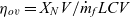
Flights A, B and C have almost identical values of descent air distance, but significantly different descent fuel burn. Flight B burned 240 kg of fuel more than Flight A during descent (0.54% of aircraft mass). Several key engine and airframe parameters derived from the FDR data are shown for Flights A, B and C for the descent phase in Fig. 7. All three descents start at above 10 km altitude at close to Mach 0.8. Flight A generally descends at a lower flight speed and lower rate of descent than Flights B and C. Note that in all cases the aircraft autothrottle and autopilot were engaged for all except the final stages of approach and landing. This means that the engine throttle is automatically controlled to maintain a demanded flight Mach number or calibrated airspeed, V CAS. For all three descents, the resulting engine OPR fluctuates in the range 5-20, spending most of the descent duration at a throttle setting above flight idle. The engine parameter plots show that when the OPR is low, the non-dimensional fuel flow rate is also low, and this corresponds to a reduced gradient in the plot of cumulative fuel use versus distance. This demonstrates that to minimise descent fuel burn, the engines need to operate at the lowest OPR possible throughout descent, and as shown in Table 2, the average OPR during descent, OPR d, increases with descent fuel burn across the three flights.
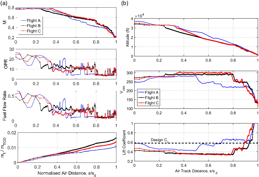
Figure 7. Comparison of descent parameters for Flights A, B and C.
The energy balance equation in Equation (2) shows that mechanical energy dissipated by airframe drag must be provided by mechanical energy from the engines and the release of aircraft gravitational potential energy and kinetic energy. The aerodynamic performance of the aircraft depends on the flight condition (Mach number and lift coefficient) as well as any airframe configuration changes. There will also be some dependency on Reynolds number, set by the flight Mach number and altitude, although this is expected to be small. Assuming a gradual descent where the lift balances the weight, the lift coefficient can be approximated at each point in the descent directly from the FDR data using the following:
 \begin{align}{C_L} = {{mg} \over {0.5\gamma {p_a}{M^2}{A_w}}}\end{align}
The plot of lift coefficient calculated this way, in Fig. 7, shows C L is generally lower in Flights B and C, and further from design, than for Flight A (the design value is taken from Ref. (Reference Vera-Morales and Hall8)). This will lead to a lower L/D value and thus a greater rate of mechanical energy dissipation due to drag, E d. This is confirmed in Figs. 8–10. For 0.5 < s/s d < 0.8, where Flight A is operating at closer to the optimum C L, this corresponds to lower OPR and lower fuel burn relative to Flights B and C, because less mechanical energy is required from burning fuel to maintain the required flight condition. The higher C L in Flight A is achieved by demanding a lower calibrated airspeed from the aircraft during descent.

Figure 8. Mechanical energy stack-up and fuel burn for Flight A.

Figure 9. Mechanical energy stack-up and fuel burn for Flight B.
The right-hand side of the mechanical energy balance shown in Equation (2) can be plotted for each point during a descent using the FDR data combined with the engine model described in Section 4. This enables the breakdown of dissipated energy to be followed in terms of GPE, KE and Efuel. The results are plotted for Flights A, B and C in Figs. 8–10, respectively. In these plots, the y-axis (the dissipated mechanical energy) has been normalised by the minimum descent mechanical energy, E d,min, as defined in Equation (12). This is the mechanical energy that would be dissipated if the air distance travelled equaled the great circle distance between end-of-cruise and the destination airport, and if the airframe aerodynamics during descent were the same as at cruise. It assumes a constant aircraft mass aircraft during descent. Also indicated on the x-axis is the great circle descent distance, s gc,d. This allows a line of minimum mechanical energy dissipation rate due to drag to be marked on each figure.
 \begin{equation}{E_{d,\min }} = {{{m_{TOD}}g} \over {{{(L/D)}_{cr}}}}{s_{gc,d}}.\end{equation}
Figures 8–10 also show the descent fuel burn, as given by the FDR, compared with what the descent fuel burn would have been if the aircraft continued consuming fuel at the same rate as during the cruise phase, as assumed by Torenbeek(Reference Torenbeek3) and determined by Equation (6). In addition, Table 3 summarises the key descent performance parameters for each flight.
Table 3 Summary of descent performance for Flights A, B and C

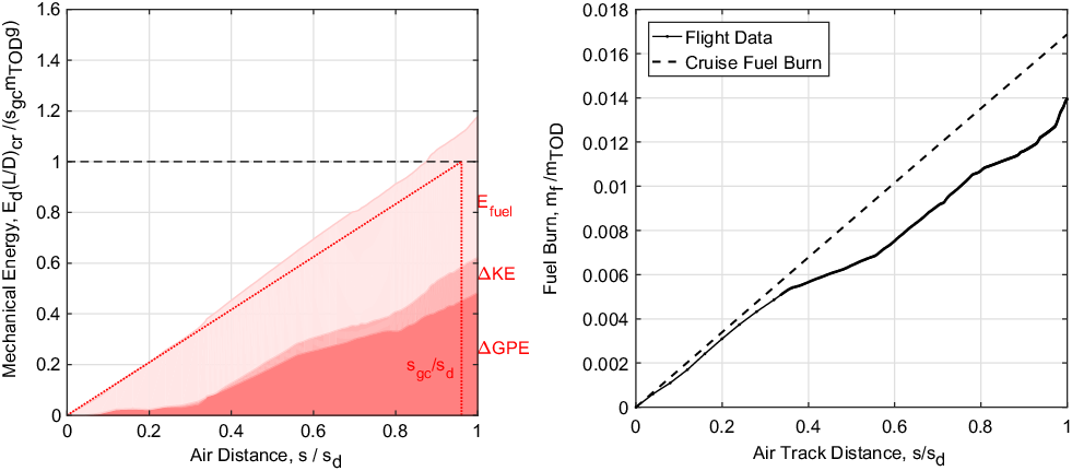
Figure 10. Mechanical energy stack-up and fuel burn for Flight C.
In Flight A, the total mechanical energy dissipated lines up well with the minimum mechanical energy required to fly the same distance, as given by Equation (12). In this case, the average L/D calculated for descent is only 5.6% lower than the cruise value. However, there is some flight-path inefficiency, with the air distance flown 12% farther than the great circle distance. Flight B has poor aerodynamic performance during descent (low L/D), giving a high rate of overall mechanical energy dissipation. The descent air distance flown is also 20% greater than the great circle distance. Flight C is in between Flights A and B in terms of total descent fuel burn. It has a descent air distance just 4% longer than the great circle distance, but poor aerodynamic performance during descent.
6.0 AVERAGE DESCENT PERFORMANCE
This section derives some averaged descent performance parameters based on flight data from all 92 A320-214 flights analysed in this study. Using the model of the aircraft engine described in Section 4, the time average overall efficiencies during cruise and descent were determined for each flight. Figure 11 shows the resulting probability density functions.

Figure 11. Probability density functions for engine efficiency during descent and cruise using data from 92 flights.
During cruise, the engines consistently operated close to a maximum overall efficiency of 31% and a Weibull probability density function was found to give the best match to the distribution of values from the flight data. This is to be expected since during cruise aircraft are operated as close as possible to an upper level of performance. In contrast, during descent, the overall efficiencies are spread over a wide range of lower values from 5% to 17%. A normal probability distribution was found to give the best fit to the data. Across all flights, the average descent overall efficiency is only 10.6% and is consistently low for all descent operations. This demonstrates how extracting mechanical energy from fuel during descent is a particularly inefficient process.
Table 4 summarises some results of the analysis across the 92 flights. The air track efficiency shows that on average, the aircraft descended an air distance 15% further than the great circle distance from TOD to touchdown. However, within the dataset, s gc,d/ s d varies from values as low as 0.62 (for descents where there are multiple periods of level holding and vectoring), to as high as 1.16 (for a direct descent with a strong tailwind). A larger value, and thus shorter descent air track distance, corresponds to less mechanical energy dissipated as drag in Equation (2).
From Equation (4), $Hg/LCV = {\eta _{ov}}(L/D)$
and therefore the average lift-to-drag ratio can be determined from dividing the non-dimensional range factor derived from the FDR data by the overall efficiency derived from the engine model. This was done for both the cruise and descent phases of each flight in order to determine the average airframe performance shown in the table. This parameter indicates that for the flights considered, L/D is reduced by an average of 13% during descent relative to cruise.
$Hg/LCV = {\eta _{ov}}(L/D)$
and therefore the average lift-to-drag ratio can be determined from dividing the non-dimensional range factor derived from the FDR data by the overall efficiency derived from the engine model. This was done for both the cruise and descent phases of each flight in order to determine the average airframe performance shown in the table. This parameter indicates that for the flights considered, L/D is reduced by an average of 13% during descent relative to cruise.
Note that the average recovered fuel for all flights is 0.22%. However, with reference to Fig. 3, for shorter descent distances, the maximum recovered fuel is up to 0.5% of the mass of the aircraft. This gives a potential maximum fuel burn saving for improved descent operation.
Table 4 Descent performance parameters averaged across all A320 flights analysed

7.0 THE FEATURES OF FUEL EFFICIENT DESCENT
The FDR data show that there is large variation in fuel burn between existing descent operations. As indicated in Fig. 5, an effective way to reduce descent fuel burn that applies to all airports and descent profiles is to reduce the descent air distance. Aircraft should therefore cruise for as long as possible before they start descent. Once in the descent phase, the aim should be to set a trajectory such that the descent air distance is as close as possible to the great circle distance and the variation of speed with altitude should be such that the airframe lift coefficient is maintained as close as possible to the value that maximises lift-to-drag ratio. This will minimise the demand from the engine for mechanical energy to balance the energy dissipated as drag, whilst still making full use of the aircraft GPE and KE. Fuel flow rate is lowest when the engines are at flight idle, and a low drag descent profile allows the engines to be set to flight idle for as much of the descent as possible. An additional factor worth considering for this is the vertical profile of wind speed. In order to further minimise descent air distance, it may be possible for aircraft to take advantage of increasing tailwinds at low altitude, for example.
As shown in Table 4 and Section 5, for flights of equal descent air distance, improvements in descent airframe performance and flight path efficiency can have significant fuel burn benefits (reductions up to 0.5% of aircraft mass). To achieve a minimum descent fuel burn both good aircraft aerodynamic performance and minimum air distance are needed. The flight data shows that such descents are possible in practice. However, a minimum fuel descent is not the minimum duration descent (since a higher lift coefficient implies a lower air speed) and in some cases could lead to significantly longer flight times. This is demonstrated in Fig. 7 where Flight A consistently has the best aerodynamic performance but the lowest corrected air speed. In addition, any descent operation is subject to the constraints of the airspace and other air traffic, which means that in practice, descent trajectories and aircraft speeds need to be adjusted in real-time. These factors require additional fuel burn, but they could be implemented whilst accounting for the impact on the airframe aerodynamics, engine off-design performance and trajectory to minimise the additional fuel requirement.
8.0 CONCLUSIONS
Based on data from 92 separate descents of A320 aircraft, total descent fuel burn can be approximated using the linear relationship ${m_{f,d}}/{m_{TOD}} = 1.4({s_d}/{H_{cr}}) - 0.0078$
. This gives an estimation of descent fuel burn that is closer to measured results than given by the fuel burn required to cruise the descent distance.
${m_{f,d}}/{m_{TOD}} = 1.4({s_d}/{H_{cr}}) - 0.0078$
. This gives an estimation of descent fuel burn that is closer to measured results than given by the fuel burn required to cruise the descent distance.
An approach for the breakdown of aircraft mechanical energy during descent has been presented based on an engine model combined with aircraft flight data. This enables engine performance, airframe aerodynamics and air track inefficiency to be isolated and compared for different descent operations.
For the Airbus A320 and CFM-56B airframe and engine combination studied, the average engine overall efficiency during descent is about one third of that at cruise, and the engine spends significant periods of time above flight idle. The descent airframe aerodynamic performance is deteriorated with an average lift-to-drag ratio that is 87% of the average value at cruise. This is a result of non-optimum altitude and speed of the aircraft during descent, leading to reduced values of lift coefficient. There are also large variations in air-track efficiency with some descents subjected to multiple periods of holding and vectoring due to ATC requirements and others closely following the great circle ground track. On average, the great circle distance was found to be 85% of the descent air distance.
To minimise fuel burn, the results from this study suggest that aircraft should cruise as far as possible before starting descent. The descent air speed and trajectory should be set such that the airframe lift coefficient is maintained as close as possible to the value for maximum lift-to-drag ratio and the minimum descent air distance. Thus, when the aircraft is flown with autopilot and autothrottle, the engine will operate at flight idle for as much of the descent as possible leading to reduced fuel flow rates and a descent trajectory that is as short as possible. The data suggests that fuel savings up to 0.5% of the total aircraft mass are possible.
Acknowledgments
The authors would like to thank Swiss International Air Lines, for provision of the flight data presented. They would like to acknowledge the support for this work from the Cambridge University Engineering Department. The authors would also like to thank Arthur Rowe, Mark Lewis, Nick Cumpsty and Ian Poll for helpful technical discussions and feedback during the preparation of this paper.


 Open access