


Introduction
The accepted definition of plasma is that in an electrically conducting medium, all paired and closely positioned positive and negative charges shield each other from an externally applied electromagnetic field (Langmuir Reference Langmuir1929). Therefore, plasma is the matter in a particular state that has the fundamental property of global electrical neutrality. The characteristic charge separation distance is the Debye shielding length and is the smallest length scale compared to all other macroscopic physical dimensions in plasma. Within this shielding sphere, the paired charged particles are not free from each other, but interact permanently, which leads to many intrinsic properties of the medium.
Charged particles in plasma interact with each other primarily by Coulomb force, magnetic induction, and collisions with neutral particles. The probability of collision can be expressed in terms of an effective momentum transfer cross-section area and the mean free path between collisions. The collision mechanism leads to the transport properties such as diffusion, mobility, and resistivity in the plasma. Plasma exists not only in gas and liquid but also in a solid conductor, except the electrons in a solid are closely bound but still can move within atomic or molecular structures between collisions. Although mass motion of charges does not generally take place, when an external electromagnetic field is applied, the dynamic effects can always be observed in electric conduction, the Hall effect, and polarization.
Plasma is electrically global neutral, and is dominated by interactions of charged particles of opposite polarity within the Debye shielding length. A strong electrostatic force exists between the paired charges; any small perturbation to the equilibrium separation distance will trigger a high-frequency oscillation by the restoring force. This oscillatory motion is referred to as the plasma frequency, which is distinguished from the lower-frequency oscillation involving mass motion. In addition, plasma does not naturally conform to its surroundings and will alter its domain according to local and distant conditions by the Coulomb force and the Lorentz acceleration. The other unique feature from the quasi-neutrality of plasma is that it stores inductive energy, and it contributes to resistance and inductance when the current circuit forms a closed loop. This characteristic is exemplified by the drastic change in electric conductivity  through a strong response to electromagnetic fields. Finally, the disturbance communication in plasma is not only by means of collision processes but also conveyed by transverse wave with phase velocities equal to the speed of light.
Plasma in the gas phase has a negligible shear stress and therefore does not have a definite shape or volume. The electric-conducting medium responds to electromagnetic fields, so plasma can be confined either by a solid container or by a magnetic field. Plasma appears in a wide range of formations such as electric arcs, filaments, micro-discharges, multiple layers in the presence of shock waves, and cellular structure in outer space. The spontaneous formations of unique spatial features on a wide range of length scales manifest the complexity of plasma. In fact, plasma is the most common state of matter by volume and is the fourth most common state of matter in rarefied and intergalactic environments. Description of plasma is therefore usually by its energy state and degree of ionization. The classification of plasma is commonly recognized by the electron number density and temperature in electron volts or the static temperature as displaced in Figure 1.1.

Figure 1.1 Classification for types of plasma.
The topics of degenerated quantum plasma and relativistic plasma are beyond the scope of plasma dynamics for aerospace engineering. Therefore, present discussions are focused on plasma that exists around atmospheric pressure, and on mixed thermal and nonthermal conditions. According to convention, the thermal condition of plasma is based on the relative temperatures between electrons, ions, and neutral components. The nonthermal or cold plasma means that the ions and neutral particles have a much lower temperature than the electrons. For most gas discharges generated by electron impact, the electron temperature is at most 3 eV (around 3 × 10⁵ 105 K), while the ions and neutrals are at near room temperature (Raizer Reference Raizer1991). When ionization is achieved by a strong shock compression in high pressure, the temperatures of the plasma composition are on the same order, around ten thousand degrees Kelvin or higher, but are not always in thermodynamic nonequilibrium. Therefore, the plasma of interest for aerospace applications is generally limited to an electron number density up to 1020/cm3 and an overall temperature lower than 106 K (Surzhikov Reference Surzhikov2013).
In engineering applications, the relative magnitude of the electromagnetic force and the inertia of gas motion have a strong bearing on the characteristics and structure of plasma. A classification of plasma by the magnetic Reynolds number becomes very important for this purpose, because the magnetic induction is generated by electric current, which is described by electric conductivity  , charge particle velocity u, and the charge number density. The magnetic Reynolds number for some characteristic scale l is defined as Rm = ulμσ in which σμ is often considered as the magnetic diffusivity and μ is the magnetic permeability of the medium. The magnetic Reynolds number has often been interpreted as a measure of the ratio of the induced and total magnetic field of the plasma. For flows with a low magnetic Reynolds number, the convection by the magnetic field lines is negligible, and the induced magnetic field by electric current is also negligible. The relationship is presented in Figure 1.2 between the electrical conductive and magnetic Reynolds numbers for most engineering applications. In general, all the assembled engineering applications presented here have the same order of magnitude in characteristic lengths and velocity scales, and the ionized gas is generated mostly by an electrical field. Thus, the magnetic Reynolds number is often much less than unity. The condition of ionosphere is included as a comparative reference, because all other astrophysical applications always have a huge physical dimension that differs from the common aerospace engineering applications. As an example, the solar atmosphere has a similar value of electric conductivity in an arc heater, but its length scale is ten million times greater and leads to a proportional greater magnetic Reynolds number (Mitchner and Kruger Reference Mitchner and Kruger1973; Shang Reference Shang2016).
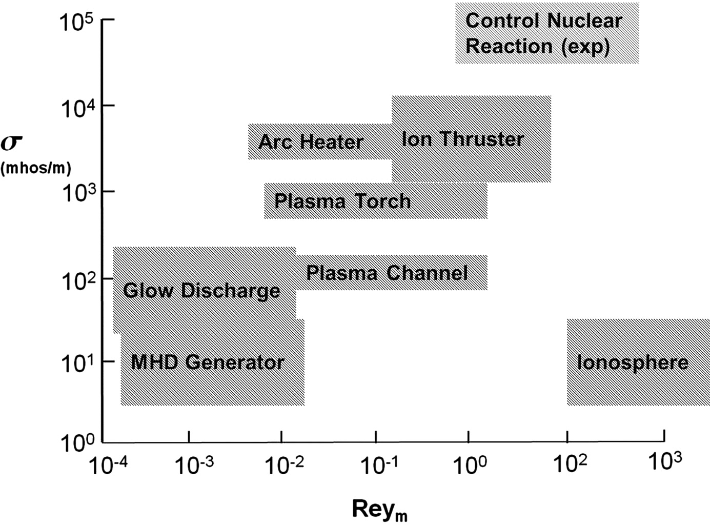
Figure 1.2 Range of electric conductivity and magnetic Reynolds numbers for common engineering applications.
All physical phenomena of plasma are governed by the Maxwell equations, but once the plasma is treated as a continuum for engineering applications, it becomes an interdisciplinary subject at macroscopic scales. The global thermodynamic and kinematic properties of plasma must be described through a distribution function between microscopic and macroscopic dynamics. This approach is accurate when the microscopic structure can be linked approximately to macroscopic motion by the Maxwell-Boltzmann distribution. However, by this approach the detailed wave-particle interaction will be unresolved.
1.1 Intrinsic Electromagnetic Forces
Plasma always exists in electric and magnetic fields. The electric charged particles interact and respond to externally applied fields and always create induced field components; the total electromagnetic field is therefore a sum of the applied and the induced components. One of two elementary electromagnetic forces arises from the attraction and repulsion of charged particles of the opposite and same polarities known as the electrostatic force. A free charged particle motion will produce a magnetic field, and when it is moving within an applied magnetic field will be compelled by the Lorentz force to accelerate in the direction perpendicular to both the charged particle motion and the magnetic field.
The electrostatic force between two singly charged particles is described by Coulomb’s law. The force between charged particles is collinear along the unit space vector between two charges separated by a distance rij as:
 (1.1)
(1.1)In Equation (1.1), the symbol  designates the unit vector between the two charged particles. The magnitude of the force is directly proportional to the product of the two electric charges and inversely proportional to the square of the distance between them. The symbol
  is designated as the electric permittivity and in the international system of units (SI) it has a value of 8.85 × 10⁻¹² Farad/m (Krause Reference Krause1953). The charges
  and
and  are measured in Coulombs, which attract each other if they are of the opposite polarity, but repulse each other if they are the same. The resulting force per unit charge is usually defined as the electric field intensity E, and the source of the electric intensity is derived from the electric charge. However, a conductor and an isolator will respond to the electric field differently. Through the definition of electric intensity; the electrostatic force can be given as:
The SI unit of the electric field intensity is the Newton per Coulomb, however, in practical application, it is often given in Volt per meter. For multiple point charges, the principle of superposition applies so the force is the sum of all other particle charges. The entire electric field of space charges is the vector sum of the entire field from all the individual source charges, in which the symbol  denotes the unit vector between the charges:
 (1.3a)
In an electrically conducting medium, the free charge particle movement will produce electric current and exert additional force on each other. In an isolator, the molecules of a dielectric material will polarize to reduce the net local field intensity. The different effects on two kinds of media are described by a dielectric constant  and Coulomb’s law becomes:
 (1.3b)
The dielectric constant  has a value of unity in vacuum and for most gas species of air. However, for isolators such as polystyrene, glass, and rubber, the constant has the values of 2.7, 4.7, and 6.7, respectively.
The free electric charge in motion produces a conductive electric current. In metallic conductors the charge is carried by electrons with an elementary negative charge of 1.61  10–19 Coulomb. In liquid conductors, such as electrolytes, the charge is carried by both positive and negative ions. The electric field compels the free charges into continuous motion and results in an electric current that can be defined in terms of the electric flux vector per unit area. The conductive current density is different from the convective and displacement current densities. The convective current does not involve an electrically conducting medium and consequently does not satisfy Ohm’s law. The convective current flows through an isolating medium such as a liquid, rarified gas, or vacuum, and the best example is an electron beam within a vacuum tube (Jahn Reference Jahn1968). The displacement current arises from the time-varying electric field and is introduced by Maxwell to account for the generation of a magnetic field when the conductive current is zero. Without the concept of the displacement current, the electromagnetic wave propagation would be impossible (Stratton Reference Stratton1953).
The conductive electric current density J has a physical dimension of coulomb per second or ampere. It is a vector for which its orientation is dictated by the vector sum of all electric particle velocities:
 (1.4)
(1.4)where ni denotes the charge particle number density and ui is the averaged velocity of the charged particles. The current charge density  is defined as the sum of the total electric charges per unit volume of species i.
A magnetic field generated by an electric current and the orientation of the induced magnetic field is defined by the right-hand rule. The current may be due to an externally applied electromagnetic field, or an electron beam, or a conductive current in current-carrying wire. Analogous to the electrostatic force, the magnetic field intensity H is defined by the field intensity at a distance r from the source. In fact, the differential magnetic field intensity is governed by the Biot-Savart law for magnetostatics, which is the counterpart of Coulomb’s law for electrostatics. The field intensity is proportional to the product of a differential current element  , direction sine of the angle between the points of interest, and inversely proportional to the square of the mutual distance. The induced magnetic field line is continuous. In vector form the Biot-Savart law gives (Jackson Reference Jackson1999):
 (1.5a)
A current-carrying wire produces a magnetic field perpendicular to the electric current, and the magnetic field strength H has the physical unit of Amp/m2. The magnetic field orientation is defined by the right-hand rule with respect to the generating electric current. Similar to electrostatics, the intermediary magnetic field variable is the magnetic flux density B or is also called the magnetic induction, which has the physic unit of Weber/m2 or Amp/m2. The connection between the magnetic field strength H and the magnetic flux density B in an isotropic medium is the constitute relation;  and
and  is referred to as the magnetic permeability. In free space, it has the dimensional value of
  Hennery/meter.
From Equation (1.5a), the magnetic flux density B therefore can be given as:
 (1.5b)
Like that of electrostatics, the force on a current element becomes:
 (1.5c)
Note that the induced forces components  and
and  are symmetric, thus opposite each in directions. However, the electric current–induced forces still can contradict Newton’s third law by the free charge movement and by the transient electric current in an incomplete circuit (Jahn Reference Jahn1968).
If two current-carrying wires are brought into the vicinity of each other, each wire is surrounded by two individual magnetic fields, leading to a force that acts on the wires. When the wires are carrying current in the same direction, the wires are attracted to each other; when the wires are carrying current in opposite directions, the wires are repelled. The interaction of two electric elements is depicted in Figure 1.3. The incremental force existing between the elements of the current path Ji and Jj is:
 (1.5d)
Basically, there are two modes of the electromagnetic body force in an electrically conducting medium that can exert on the charged particles. The interaction of the electric field with the free charge density of the medium  is known as the electrostatic force. The interaction with an externally applied magnetic field by an electric current that is driven by a force within the medium is
  , known as the Lorentz force, both Fe and Fm have the physical unit of Newton per meter square. From Equation (1.4), the current density is directly related to charge particle motion then
  and it is the well-known Lorentz force. It is also often considered that the electromagnetic or Lorentz force is
  .
.

Figure 1.3 Induced magnetic force by two electric current elements.
1.2 Charged Particle Motion
The moving charged particles in an electrostatic field will induce a magnetic force perpendicular to the orientations of the applied electric field; therefore these are always associated with an electromagnetic field. According to Coulomb’s law and the Biot-Savart law, the motion of an electrically charged particle always consists of a rectilinear and rotational component. The rectilinear acceleration is aligned with the externally applied electric field and a gyration intrinsically revolves around an induced and applied magnetic field vector. In the absence of an electric field, the angular acceleration is restricted in the plane perpendicular to the magnetic field. A moving charge q with a velocity u in a steady and uniform electromagnetic field with an applied magnetic flux density B will be pushed by a force normal to B, and also directly accelerated by the electric field intensity E. The force that is perpendicular to the directions of the charged particle velocity and the magnetic field is the Lorentz force or acceleration,  . As a consequence the equation of motion for a charged particle with a velocity of u in an electromagnetic field is:
 (1.6a)
If the electric field is negligible, the magnetic flux density is applied along the z-coordinate. Under this circumstance, the motion of a charged particle along the z-coordinate is unaltered, thus the normal force component of the charge particles is always restricted in the plane perpendicular to a constant and steady magnetic B. The velocity components in three-dimensional space can be combined into the component that is parallel  and perpendicular
  to the magnetic field. The velocity component
  that is parallel to B will not be affected by the magnetic field, but the velocity component
  normal to B will gyrate around it. The scalar components for the equation of a charge motion in the x-y plane perpendicular to an applied magnetic field and aligned with the z-coordinate becomes:
 (1.6b)
Here and further:

are the unit vectors of the Cartezian reference system. The general solution to the first-order partial differential equation in time; Equation (1.6b) is:
 (1.6c)
In Equation (1.6c),  the symbol
  is denoted as the electron cyclotron frequency or the Larmor frequency as (for electron e=|q|):
 (1.6d)
Using Equation (1.6d) for calculating the Larmor frequency of a single charge, the magnetic flux density B needs to be in the SI unit of Weber/m2.
Equation (1.6c) actually describes the single charged particle motion by a simple harmonic oscillator with the cyclotron or Lamor frequency. The trajectory of the charged particle in a pure magnetic field can be obtained by integrating the equation of motion, Equation (1.6c), and taking the real component of the results to get the location of the particle in the x- and y-coordinates:
 (1.6e)
As before by defining a gyro radius as  , the charge particle motion in the normal plane to the magnetic field must follow a circular path and the charged particles will execute a spiral motion. The gyro radius can be determined easily by the balance of the centrifugal acceleration and the electromagnetic force exerted on a singly charged particle,
  . The radius of the circular motion of a group of charged particles in the plane perpendicular the magnetic field is
  , with an angular gyro velocity
  . In short, the gyro radius is often referred to as the Larmor or cyclotron radius and can be evaluated based on a single electron,
  . Similarly, the rate of the angular gyro velocity has also been widely referred to as the Larmor or cyclotron frequency. The charge particle trajectory in a three-dimensional electromagnetic field is then a helix with its axis parallel to B and a pitch of
  . When the electric field vector is applied in addition to the magnetic field, the charged particles will execute a persisted spiral trajectory as shown in Figure 1.4. The orientation of the resultant helical trajectory is dictated by the direction of the applied electric field intensity. In fact, the direction of gyration is opposite to the applied magnetic field and tends to reduce the applied magnetic field strength, a process known as diamagnetism.

Figure 1.4 Trajectory of electron motion in electromagnetic field.
In a steady state the electromagnetic force components are balanced; thus from Equation (1.6a) we shall have  . By taking the cross-product with respect to B of the equation, using a vector identity,
  and recognizing that
  , it yields:
 (1.6f)
The resultant velocity  is the well-known drift velocity of
  , which moves in a direction perpendicular to both the electric and magnetic fields. The drift velocity leads to the well-known Hall effect (Hall Reference Hall1897).
Meanwhile, in a magnetic field that is increasing in strength, the kinetic energy parallel to the field converts into rotational energy of the particle and increases its Larmor radius. However, the energy of the system is invariant because the magnetic field does no work to change the total kinetic energy of the charged particle. When the magnetic field increases to a point, the velocity parallel to the magnetic field vanishes; it leads to a unique phenomenon of the magnetic mirror for plasma by the Lorentz force (Goldston and Rutherford Reference Goldston and Rutherford1995; Goebel and Katz Reference Goebel and Katz2008).
In a large group of charged particles, the charged particles will encounter numerous collisions with each other and neutrals in partially ionized plasma. The charged particles’ dynamics are untraceable, but the global behavior for the system of particle has been thoroughly studied by the field of statistic thermodynamics. The global effect of collisions can be determined by the velocity distribution function for each species in the microscopic motions to the macroscopic behavior of plasma. In the absence of the other forces, these particles can be characterized by a speed solely as a function of the group temperature and mass of the species. The most probable distribution of velocity in thermal equilibrium is the Maxwell distribution:
 (1.7a)
Where k is the Boltzmann constant, in SI units  , and in plasma dynamic applications the value of
  is frequently used. In Boltzmann distribution Equation (1.7a), the notation T is the system temperature in a thermal equilibrium state. From this distribution function, the average velocity of the system can be found as:
 (1.7b)
The classic result of the average velocity of a particle in a thermodynamic equilibrium state is obtained by integrating Equation (1.7b), which is proportional to the square root value of the temperature and inversely proportional to the unit mass of the particle. The result reveals the huge difference between the average velocities of electrons and ions due to the difference in masses of electrons and ions.
 (1.7c)
It becomes clear that the stationary charges generate an electrostatic field; in fact, the remotely acting Coulomb force is the genesis of the intrinsic characteristics of plasma for the Debye shielding length and the plasma frequency. While the direct current produces a magnetostatic field, the dynamics of the electromagnetic field must more often be accompanied by a time-varying electric current density. In short, within a static electromagnetic field, the electric and magnetic fields are independent from each other, whereas in dynamic states the two fields are interdependent.
1.3 Debye Shielding Length
Two fundamental parameters associated with the electric properties of plasma are the Debye length and the plasma frequency; both characterize the macroscopic behavior for a collection of charged particles. The basic property of plasma is its tendency to maintain electric neutrality (Langmuir Reference Langmuir1929). This particular state requires an enormously large electrostatic force between an electron and ion. A quantitative estimate of this dimension over which a deviation from charge neutrality may occur can be obtained by the Gauss law for electric field,  . The physical meaning of this law simply states that the property of the electric displacement is determined by the local electric charge density. The electric displacement is related to the electric field intensity by a constitutive relationship,
  , where
  is the electric permittivity. In a homogeneous field and isotropic medium, the electric field intensity is inversely proportional to the gradient of the electric potential,
  . The resultant equation is known as the Poisson equation of plasma dynamics:
 (1.8a)
In a thermodynamic equilibrium state, the number densities of electrons and ions are given by the Boltzmann distributions, and by invoking the fact the plasma is electrically neutral; namely, ni = ne.
 (1.8b)
Substituting these expressions into the Poisson equation of plasma dynamics and reducing the equation to a one-dimensional problem:
 (1.8c)
Expanding the exponential function of the right-hand side of the equation by Taylor series in ascending order of  gives:
 (1.8d)
Although the magnitude of  may not be necessarily negligible over an entire domain between charged particles, the potential is known to drop rapidly with respect to the separation distance between the charged particles. Therefore, it is permissible to keep only the leading term, then:
 (1.8e)
It is recognized that Equation (1.8e) is a simple harmonic equation; the general solution is:
 (1.9a)
The electric potential of Equation (1.9a) reaffirms an exponential decay behavior as a function of distance between charged particles, and can be given as:
 (1.9b)
Equation (1.9b) leads naturally to the definition of the Debye shielding length. This is the minimum and defining characteristic length scale for plasma, and within this space a pair of electron and ion isolates each other from the external electric field.
 (1.10a)
In practical applications, the Debye length can be calculated easily by:
 (1.10b)
In Equation (1.10b), the Debye shielding length is given in meters. The input electron number density and temperature are required to be number per cubic meter and in electron volts only. The temperature of the free-electron component of the gas Te is not necessarily equilibrated with the ions or neutrals of the plasma. The Debye length has always been adopted as an index of the typical charge separation distance in plasmas that are sustained by the random thermal energy of the electrons. These simplified results for the Debye length by Equation (1.10b) are evaluated by the following constants: electron volt (1 eV = 1.1604 × 10⁴ K); Boltzmann constant of 1.3807 × 10⁻¹⁶ erg/K; elementary charge of 4.8032 × 10⁻¹⁰ Coulomb; and electric permittivity of free space 8.8542 × 10⁻¹² Farad/m.
The typical value of the Debye length in a magnetohydrodynamics (MHD) generator is in the same order of magnitude of the electron mean free path O(10–6 – 10–7 m) at a temperature of 2,500 K and charge number density of 1020/m3. In plasma generated by electronic impact at standard atmospheric conditions, the Debye length is 1.14 × 10⁻⁷ m.
A most illustrative phenomenon of Debye shielding length is the plasma sheath. The charge neutrality of plasma does not prevail in the immediately adjacent region to a solid surface, especially over electrodes of an externally applied electric field. The boundaries of the plasma represent a physical interface through which energy and charged particles enter and leave the plasma; the plasma will establish the potential and density variations at the interface to satisfy charged particle balance or by the imposed electrical boundary. The narrow domain surrounding the media interface is the so-called plasma sheath. The Debye length gives the order of magnitude for the thickness of the sheath that separates the neutral plasma from an interface. Under this circumstance, by a first-order analysis for quasi-neutrality, the ratio of the electron to the ion current density at the interface is:
 (1.11a)
The ratio of current density on the interface can be further developed by the conservation law of energy for the charged components of the plasma,  and
and  , to yield:
 (1.11b)
Recall that the mass ratio between ion and electron is at a value greater than one thousand to one. In general, electrons left the plasma volume faster than ions because of a greater mobility; a charge imbalance would generate a positive electric potential at the interface. This physical characteristic is easily identifiable in the cathode and anode layers of a glow discharge that is generated by a strong electric field. Another contributing factor to this behavior is the recombination mechanisms of chemical kinetics by depleting the charges of ionized gas when striking the surface. The electron absorption and emission properties of the solid surface also play an important role. This phenomenon is closely related to the catalytic of the surface material.
The computational simulated direct-current discharge duplicating the experimental observation is depicted side by side in Figure 1.5. The discharge is generated between parallel metallic electrodes with a gap distance of 1.0 cm and the external electric potential is applied by a voltage of 400 volts under an air ambient pressure of 10 Torr. The total current of the charge is measured to be 10 mA. The detailed discharge structure from the experiment is overwhelmed by the emission or the glow in the photography record, but the cathode layer is clearly captured by the computational simulation. The numerical result displays the positive discharge column over the cathode layer; the plasma sheath is well formed by the cathode fall. The computational result is presented by twenty uniformly increment electron number density contours with a maximum value of  .
.

Figure 1.5 Cathode layer of a DC parallel discharge  .
.
1.4 Plasma Sheath
The plasma sheath is another unique feature of plasma at the interface of different media, which is directly connected to the vastly different unit mass between the electron and ion. For a hydrogen atom the ratio of an ion to electron is 1,836 to one. Away from the media interface the bonded electron and ion must move at the same speed to maintain the global neutrality. Near the boundary, charge separation occurs and the charged particles tend to move at different random motions. The average electron and ion velocities at thermodynamic equilibrium condition according to the Maxwellian distribution are:
 (1.12a)
 (1.12b)
The electron and ion mass flux vectors,  , are given as:
 (1.12c)
 (1.12d)
Therefore if the temperatures of electrons and ions are equal, the average velocity of an electron is at least forty-two times greater than that of ion. However, in an electron-impact plasma generation process, the electron temperature is much higher than that of the ion to make an even greater disparity. In free space and without the presence of an electric field, the electron and ion pair in plasma is restrained from a separation distance of the Debye shielding length to each other by the electrostatic force. Near the interface boundary, charged particles separate; the higher collision rate of electrons with a surface is much greater than ions to make the surface acquire a net negative potential (Riemann Reference Riemann1991). The ions will recombine at the surface and return the plasma to neutral particles; the electrons either recombine or enter the conduction band for an electric conducting material. Most important, the plasma loses the globally neutral property in this region and the electric potential increases monotonically toward a negative value from the unperturbed neutral state. When the collision process reaches an equilibrium state, the net electric current at the interface surface vanishes. A plasma boundary layer is formed over the interface known as the plasma sheath. It may be anticipated that the plasma sheath often has the same order of magnitude of the Debye shielding length.
The thickness of a plasma sheath is dependent greatly on the interface surface recombination rate and the curvature of the surface, thus the plasma thickness is problem dependent and it is difficult to provide a general solution. However, on a flat interface surface the electric potential and the inner structure can be estimated by neglecting the drift velocities of the charged particles and assuming the electrons and ions have the same temperature and under thermal equilibrium condition. Under the stated condition, the number densities of charged particles are Maxwellian:
 (1.13a)
 (1.13b)
At the considered condition, there is no net charge building up on the surface:
 (1.13c)
The zero surface charge condition for an electrically conducting flat surface is implemented by substituting the mass flux densities of electron and ion  and
and  , Equations (1.12c) and (1.12d), into Equation (1.13c) to get:
 (1.13d)
The estimated electric potential in the plasma sheath becomes:
 (1.14)
The estimated plasma sheath potential (Bittencourt Reference Bittencourt1986) surprisingly reaches a qualitative affinity with more accurate analysis. At the present, the plasma sheath and electric potential immediately next to the interface can be routinely calculated by numerical simulation utilizing the classical drift-diffusion theory. In the case for simulating the direct current discharge, the secondary emission from the cathode surface has also been taken into consideration.
As an example, the electric field strength distributions in the positive column between the anode and cathode of a direct current discharge are displayed in Figure 1.6. The typical cathode sheath is clearly displayed; in a direct current discharge, the electrons carrying most of the current in the positive column now are prevented from reaching the cathode, and the massive ions are incapable of carrying the total current. The discharge is maintained by the secondary emission of electrons by the bombardment of incoming ions, leading to the exponential growth of electron density and flux from the cathode. The value of the exponent is known as the first Townsend coefficient (Lieberman and Lichtenberg Reference Lieberman and Lichtenberg2005). In Figure 1.6, the numerical results are obtained for three different ambient pressures. Three discharges are generated at a fixed electrodes gape distance of L = 2.00 cm between metallic electrodes from ambient pressures from 3.0, 5.0 to 10.0 Torr. The electric potentials are required to increase from 417.6, 534.0 to 826.1 Volts to maintain the discharge for the elevated pressure. On the other hand, the discharge currents decrease from 5.27, 4.88 to 3.9 mA as the ambient pressure is elevated. The computational simulations reveal that the electric field intensity is nearly constant across the positive column but increases rapidly in both the anode and cathode layers. The electric intensity drops drastically from the cathode surface toward the positive column for all three ambient pressures simulated to display the distinctive behavior of cathode fall. The electric field strengths at three different ambient pressures show a monotonic drop by two orders of magnitude from the cathode surface. The plasma sheath of the discharge is also more noticeable in the cathode layer than in that over the anode. The pressure or density of the discharges exerts little influence on the thickness of the plasma sheath, because the sheath thickness is dependent strongly on the charged number density. For the direct current discharge, the electron number density is sustainable at a nearly constant and maximum value of 1010/cm3. Under the higher-density environment, the plasma sheath is slightly thinner, but the steep electric potential gradient remains.

Figure 1.6 Electric field structure in direct current discharge.
1.5 Plasma Frequency
Plasma has a tendency to be macroscopically neutral; the relative position of paired charges will always return to its neural equilibrium state after a perturbation. The inertia of electrons will unavoidably lead to overshoot and oscillate around the equilibrium condition by a characteristic rate known as the plasma frequency. The plasma frequency is therefore a measure of a time scale of restoring forces that exerts on a displaced electron returning within Debye length to an ion and keep plasma to an electrically neutral state. In the absence of a magnetic field and without externally applied thermal perturbation, the coupled ion can be considered in a fixed location in uniform plasma that extends to infinite (Mitchner and Kruger Reference Mitchner and Kruger1973). The mass and momentum conservation equations of electron motion in one dimensional case are:
 (1.15)
The compatible electric field E can be determined by the classic Poisson equation of plasma dynamics in one-dimensional formulation:
 (1.16)
The system of equations can be solved easily with a linearized perturbation approach by setting the known initial conditions and considering the displaced electron as a small disturbance:
 (1.17a)
In Equation (1.17a) Eo, uo, and no denote the equilibrium values of the electric field, electron, and number density of the electron. At the equilibrium quasi-neutral condition, the uo and the rate of change of no shall have null values.
Substituting the perturbation series of Equation (1.17a) into Equation (1.16) and collecting the terms of order of O( ), the resultant linearized governing equations become:
 (1.17b)
The perturbed oscillating variables are naturally definable by simple harmonic functions:
 (1.17c)
Substitute these general solutions into the governing equations, Equation (1.17b), and eliminate n1 and E1 to get:
 (1.17d)
From Equation (1.17d), the square value of the wave number is found as  . The plasma frequency is therefore:
 (1.18)
The plasma frequency is one of the fundamental parameters of plasma, and the inverse value is approximately the minimum period for plasma that reacts to changes caused by an applied electric perturbation. For plasma with a number density of  or
or  , the plasma will respond to a perturbation in less than a nanosecond. The practical approximate formula of the corresponding circular frequency in SI units is:
 (1.19)
The pertinent parameters for the plasma frequency calculation are the electric permittivity in free space  = 8.8542 × 10⁻¹² Farad/m, the elementary charge e = 1.6022 × 10⁻¹⁹ Coulomb, and the electron mass m of 9.1095 × 10⁻²⁵ g (Raizer Reference Raizer1991).
For an example, the electron number density in an electron-impact discharge has a value of around 1018/m3 or 1012/cm3. The plasma frequency yields a value of 8.7 × 10⁹ Hz, which is within the H and X bands of the microwave frequency. In other words, the plasma will respond to any electrical perturbation in less than a nanosecond. The frequency, however, is lower than the typical average electron collision frequency 2 × 10¹¹ Hz within a plasma generator in an externally applied electromagnetic field.
1.6 Magnetohydrodynamic Waves in Plasma
An ionized gas can generate a wide variety of oscillatory motions. Three types of waves in plasma have been classified as electromagnetic, hydromagnetic, and electrostatic (Spitzer Reference Spitzer1956). However, it is most unlikely all of these idealized waves can exist in their pure form. The electromagnetic waves in the simplest cases are only transverse waves that are associated with the transverse motion by lines of magnetic induction. The tension in the lines of magnetic force tends to restore deformation back to the original state. These waves are exemplified by electromagnetic waves propagating in vacuum (Friedrichs and Kranzer Reference Friedrichs and Kranzer1958), and the phase velocity is on the order of the speed of light. Hydromagnetic or magnetohydrodynamic waves are similar to acoustic waves, which are low-amplitude, longitudinal, compression motions through collisions and are concurrently produced by the electromagnetic coupling of the electrons and ions. The wave propagation speed is governed by the speed of sound. Finally, electrostatic waves are also a longitudinal wave and propagate due to thermal agitation (Landau and Lifshitz Reference Landau and Lifshitz1960).
The time-dependent, three-dimensional Maxwell’s equations govern the propagation of all electromagnetic waves. In order to describe wave motion for the purpose of better understanding, the plasma is considered as an unbound isotropic and stationary medium. The wave equation in plasma is derived by taking the temporal derivative of the generalized Ampere circuit law to get:
 (1.20a)
Then replace the time derivative of the magnetic field strength H by Faraday’s induction law for an isotropic medium  and
and  by the constitutive relationship; we will have:
 (1.20b)
Finally, invoke the following vector identity and substitute it into Equation (1.20b)
 (1.20c)
We have the basic electromagnetic wave equation in time and space:
 (1.20d)
In discussing the wave motion, the orientation of the particle motion is relevant. The identical wave equation for a plane wave with the magnetic field strength H is obtainable by the same combination of Faraday’s induction law and Ampere’s electrical circuit law, in an electromagnetic field with a uniform electric intensity and without electric current. The resultant equations system is referred to as the D’Alembert equation:
 (1.21a)
It is immediately noticed from Equation (1.21a) that the electric and magnetic wave components oscillate in synchronization but perpendicular to each other. The energy transfer by a traveling electromagnetic plane wave can be evaluated by the electric and magnetic energy density by the Poynting vector,  (Stratton Reference Stratton1953). Therefore, the oscillations of two field components are orthogonal to each other and perpendicular to the direction of energy and wave propagation. This phenomenon exemplifies the intrinsic property of a transverse wave. In these waves, the frequency is very high and the ions are unaffected by the electric field and the electrons retain the Boltzmann distribution. In a vacuum, the wave propagation at the speed of light is
  .
.
The electromagnetic wave propagates in a dielectric without impendent, but will completely reflect at the interface between free space and plasma, when the incident electromagnetic wave frequency is lower than the plasma frequency. The electromagnetic wave can propagate through plasma when the incident wave possesses a higher frequency than that of plasma but with attenuation. Electromagnetic waves will dissipate rapidly in an electrically conducting medium; the penetration depth is dependent on the incident wave frequency and electric conductivity of the conductor. These behaviors are manifestations of Debye shielding effects from the response by the paired charges to the externally applied electromagnetic field.
The electromagnetic waves in time-harmonic mode usually are given as:
 (1.21b)
where k is designated as the wave number, for the plane wave it is a vector that is normal to the wave front, and  is the so-called angular frequency. The wave amplitude is a dependent of the wave frequency,
  . Thus the functional relationship between these parameters is referred to as the dispersion relationship, which is the properties of the transmitting medium. The ratio of
  has a specific meaning in wave propagation; it is called the phase velocity of the wave, and for an electromagnetic wave it has the magnitude of the speed of the light.
Figure 1.7 shows the projected electric flux and magnetic flux density contour lines of a transverse electromagnetic wave propagating in a square wave guide. A comparison is also made for computational results with analytic solutions for the entire electromagnetic field for waves traveling along the z-axis. In a cross-sectional plane (x-y) of the waveguide, the electric field is traced by solid lines and the magnetic field is depicted by dots. The affinity between the analytic and numerical results is identical within plotting error. The instantaneous contours of an electromagnetic wave clearly illustrate that the electric and magnetic components of the transverse wave are propagating perpendicularly to each other and in phase. The orthogonal condition is maintained between the electric and magnetic fields over the complete length of the waveguide.

Figure 1.7 Contour lines of a transverse electromagnetic wave in a waveguide,  .
.
The electric charge in the electrostatic wave is due to the divergence of the current density. There are two types of oscillations, namely the electron and ion oscillations. How the electron oscillations are excited in plasma is not clear, but these waves are damped as the wavelength approaches the Debye shielding length. The positively charged ion oscillations are waves of relatively low frequency. The electrical neutrality is preserved and the electrostatic wave usually behaves as an acoustic wave.
The hydromagnetic wave appears only in the presence of a magnetic field and at frequencies lower than the cyclotron frequency of the ions. The driving mechanism is the Lorentz acceleration  , and the amplitude of oscillation is conserved in the line of magnetic force. The basic form is known as the Alfven wave, which is a purely magnetohydrodynamic phenomenon depending on the magnetic field and inertia of the medium. The wave velocity and the induced magnetic flux density are parallel to each other while the mean magnetic field is normal to them. For the Alfven wave (Alfven Reference Alfven1950), the divergence of the medium velocity vanishes and the pressure gradient term becomes zero. For these reasons, the pressure and density do not vary in such transverse waves. Therefore transverse wave motion is possible in an incompressible medium.
The phase velocity of these waves is the Alfven speed that is based on the component of the applied magnetic field in the direction of the wave propagation. From this viewpoint, the Alfven wave is the vibration by a line of force. Its phase velocity is:
 (1.22a)
The normal stress component associated with lines of force is the well-known Maxwell tensile stress BB.
When electric field intensity is perpendicular to the wave front, it will lead to an electromagnetic wave reaction. The electrons will interfere with these transverse waves and increase the wave speed. When the electron number density exceeds a critical value with increasing plasma frequency, the electromagnetic wave cannot propagate through the plasma in the presence of an electromagnetic field. Another characteristic of wave motion in plasma is that the waves can propagate by different phase speeds. Since transverse waves can exist both in a compressible or an incompressible medium, the electromagnetic waves in a compressible medium have been referred to as magnetoacoustics waves (Sutton and Sherman Reference Sutton and Sherman1965). Two phase velocities uf and us corresponding to the fast and slow magnetoacoustics waves are:
 (1.22b)
The phase velocities are dependent on different angles between the applied magnetic field and the direction of wave propagation. The velocity of the fast wave is always greater than the Alfven wave speed, and that of the slow wave is always less than it. The phase velocities of the electromagnetic waves degenerate to the speed of sound when the transverse magnetic field vanishes.
1.7 Landau Damping
Landau damping relates the electric field decay of an electromagnetic wave by phase mixing in which charged particles follow the angular velocity of a perturbation at a fast spatial oscillation. The temporal decay of wave amplitude of a longitudinal electromagnetic wave takes place in the absence of a dissipative mechanism such as the collision process with other particles. Therefore, it is the result of unique electron interaction with an electric field of electromagnetic wave, and the phase velocity of the wave becomes the key issue. The best approach to understanding Landau damping is by finding an approximation expression for the dispersion function that relates the propagation coefficient  and angular frequency
  of a general solution from the macroscopic self-consistent electric and magnetic fields equations (Landau Reference Landau1946; Landau and Lifshitz Reference Landau and Lifshitz1960). As always, the starting point for most classic work is the Maxwellian distribution, which is an accurate distribution for stationary equilibrium plasma:
 (1.23a)
The dispersion relationship for a longitudinal electron wave can be found by applying the Maxwell distribution function by method of moment (Landau and Lifshitz Reference Landau and Lifshitz1960; Bittencourt Reference Bittencourt1980):
 (1.23b)
For the condition that the value of  is much greater than unity, and by an asymptotic expansion the following dispersion relation is obtained at the high phase velocity limit:
 (1.23c)
The complex angular frequency can be separated into the real and imaginary part as  , and by defining
  :
:
 (1.23d)
For a standing wave where the complex wave number is real, the negative imagery part of the angular frequency will lead to the temporal decay because the wave motion is described by the general solution:
 (1.23e)
The damping of a longitudinal plasma wave was first discovered by Landau (Landau Reference Landau1946), and Equation (1.23d) is referred to as the landau damping factor. The decay of a longitudinal plasma wave by Landau damping is not the usual dissipative mechanism via the collision of electrons with heavy particles, but rather arises from the interaction between the electron’s interaction with the electric field. This phenomenon takes place when the electron moves very close to the phase velocity of the longitudinal wave, and the electrons are trapped within the potential wells of the propagating wave.
In collisionless plasma, the Maxwellian distribution function describes electron velocities fairly accurately. When an electron moves at the outer edge of the distribution function moving slightly slower than the wave phase, velocity will gain energy from the wave. The direction of energy exchange between an electron and the electromagnetic wave will reverse for electrons moving slightly faster than the wave phase velocity. Therefore, Landau damping occurs when the number of slower-moving electrons is greater than the faster-moving electrons in respect to the wave phase velocity. Specifically, Landau damping will take place when the wave number k is close to a value inverse to the Debye shielding length, the electron velocity band  near phase velocity
  . Under this circumstance, there are more electrons in the velocity band initially slower than the phase velocity than electrons that are faster than the phase velocity. The trapped electrons in the potential well will gain electron energy at the expense of the wave energy; Landau damping happens in the region where
  or the slope of the distribution is negative. Under an unstable condition, the amplitude of an electromagnetic wave will grow with time when
  . In fact, Landau damping prevents instability from developing and is also a manifestation of the mathematical property of electron and electromagnetic wave interaction when the electrons move near the phase velocity of the wave.
1.8 Joule Heating
Joule heating is also known as Ohmic and resistive heating. The phenomenon arises from interactions between moving charged particles through collisions. The resulting scattering motion from elastic and inelastic collisions is completely random to become thermal energy. It is the process by which the passage of an electric current through a medium releases heat. In other words, the electromagnetic field does work to overcome the resistive force that equals to the dissipated energy due to resistance. The amount of energy released is proportional to the square of the current. This relationship is known as Joule’s first law and the IS unit of the energy was subsequently named after Joule by the symbol J (J = 1 Newton-meter, or J = 107 erg in SGS).
Joule heating is the consequence of the interaction of charged particles in an electric circuit accelerated by an electric field, but electrons must give up some of their kinetic energy every time they collide with ions of the conductor. The increase in kinetic or vibrational energy of the ions manifests itself as heat and an elevation in the temperature of the conductor. In steady state, the electron momentum equation including the electron–ion and electron–neutral collision can be approximated as:
 (1.24a)
where  and
and  characterize the collisional frequencies of electrons with ions and with neutral particles, respectively. Since the electron velocity is so much greater than that of neutral, the foregoing equation can be approximated as:
 (1.24b)
By neglecting the collision frequency of electrons and neutrals in comparison to the collision between electrons and ions, and by the negligible partial pressure gradient of electrons, Equation (1.24b) is simplified. Recall the total electric current is defined as  , and
, and  is the electric current of electrons; we have then:
 (1.24c)
Equation (1.24c) is known as the approximate Ohm’s law for partially ionized plasma, and the group of parameters  is the electric resistivity of partially ionized plasma. It is the reciprocate of electric conductivity
  . In the absence of an externally applied magnetic field, the most general and fundamental formula for Joule heating is:
 (1.24d)
The electric current in a circuit is the volumetric integral of the electric current density:
 (1.24e)
The time-averaged Ohmic power per unit area has been given as (Lieberman and Lichtenberg Reference Lieberman and Lichtenberg2005):
 (1.24f)
Recall that at low ambient pressure, the Ohmic heating is small in comparison to the stochastic heating. However, the Ohmic heating is dominant at high pressure due to the high collision frequency. The total energy dissipated in the conductor in time is then  and known as Joule’s law. An identical formula can also be used for alternating current (AC) power, except the parameters are averaged over one or more cycles. In these cases of a phase difference between I and E, a multiplier
  must be included.
As an example of Joule heating in a direct current discharge, a side-by-side electrode configuration is presented in Figure 1.8. The composite graph includes the computational simulation and the photograph observation under identical conditions; the gap between the cathode (on the left) and the anode is 1.5 cm. Each electrode has a length of 0.5 cm and a width of 0.25 cm. The discharge is maintained by an electric potential of 439.0 V, a discharge current of 5.2 mA at an ambient air of 5.0 Torr. The experimental observation shows intensive glows over the closest edges of electrodes. As can be seen from the numerical simulation, the electric field intensifies at the sharp edge of the electrodes. The electron number density has a maximum value of 1.7 × 10¹⁰/cm3 locally, and this value is 3.5 times greater than the infinite parallel electrode counterpart. At the inner edge of the anode, the anode layer is completely distorted by the stronger local electric field. From the contour presentation, the cathode layer can be clearly discerned even through the discharge structure over the cathode and is no longer uniform. The plasma sheath is clearly displayed in the cathode layer, and the current density is highly concentrated over the cathode. Thus, the Joule heating is concentrated along the inner edge of the cathode layer closest to the anode, at a total applied direct current electric power of 21.52 j/cm2s, the Joule heating of the glow discharge at the pressure of 5 Torr is estimated to be 1.30 j/cm2s (Shang et al. Reference Shang, Huang, Yan and Surzhikov2009). This rate of Joule heating amounts to 6.04 percent of the total plasma generation power input.

Figure 1.8 Direct current discharge over a side-by-side electrode arrangement  .
.
1.9 Plasma Kinetics Formulations
The charged particles of partially ionized plasma involve a large number of collisions between electrons, ions, and neutral species. The net effect of collisions is obtainable by applying a distribution function of the velocities for each species. In the absence of other forces and on the average, each particle will move with a speed that is a unique function of the macroscopic temperature and mass of the species. The statistical behavior of charged particles thus can usually be described by different velocity functions; the random motions are usually evaluated by taking the moments of the distribution functions. As introduced by Equation (1.7a), the most probable three-dimensional velocity distribution function for a group of particles in thermal equilibrium is the Maxwell equation:
 (1.25)
The average speed per particle is  , which is the well-known result from the kinetic theory of gas. Any flux variables are obtainable by taking the higher-order moment of the distribution function. For example, the conservation momentum equation is acquired by taking the first-order moment with the distribution function, and includes the Lorentz force:

 (1.26a)
The resultant momentum conservation equation is:
 (1.26b)
The first term of the right-hand side of Equation (1.26b) is the externally applied Lorentz force and the second term is partial pressure gradient. The pressure gradient in general should be a stress tensor, but in an anisotropic medium it reduces to a normal vector. The pressure is then given as a scalar partial pressure of a species,  . The resultant pressure force is given as
  . The momentum transfer by binary collisions between different charges and the collisions with neutral particles generates a force due to collisions that can be expressed as
  . The collision frequency is designated as
  ; the characteristic velocities of species i and j are denoted as
  and
and  .
.
The conservation of energy equation is obtained by taking the second moment with the distribution function.
 (1.27a)
The general form of the energy equation for charge species by neglecting viscous heating of the species has been provided by Goebel and Katz (Reference Goebel and Katz2008):
 (1.27b)
where the transport energy includes the work done by the pressure, the macroscopic energy flux, and heat transfer by conduction,  . The coefficient of thermal conductivity of a species given in SI units is
  , and the temperature needs to be specified in electron volts. The mean energy change by collision is
  , and Q and
  are energy exchange from elastic collisions and energy lost by inelastic collisions.
Technically, the plasma kinetic formulation has assumed that the plasma can be treated as an isotropic electrically conducting medium with Maxwellian distribution. Only the interactions and motions of all the fluid elements are considered, and the link between the macroscopic and microscopic properties is based on the most probable states.
1.10 Electric Conductivity
The electric and magnetic fields in plasma always produce an electric current that is related to the drift or diffusion velocities of the various charged particle species. Therefore, it is necessary to evaluate the electrical conductivity as microscopic properties together with the thermodynamic state of the plasma. Between collisions, the individual particles move in accordance to the  drift and diffusion velocities that are the driving mechanisms for the charged particle motions. The electrical resistivity is the resultant phenomenon of the collision process. By introducing a mean or drift motion of the electrons in the gas, the electric current is:
 (1.28)
where m is the mass of the electron and  is the average electron collision frequency, which is related to the atomic momentum transfer cross-section and the random thermal motions of the individual particles. The current density is related empirically to the applied electric and magnetic fields by a bulk electric conductivity
  . The proportional constant is known as the electrical conductivity:
 (1.29)
In fact, it is the reciprocal of the electric resistance that has the SI unit of Ohm-meter and is a function of the medium temperature. The electrical conductivity is expressed in the reciprocal of the ohm-meter, or mho. Note that Ohm’s law at a point is  , that J and E have the same direction in an isotropic medium and in the absence of a magnetic field. Under this special circumstance, electrical conductivity is a scalar quantity.
The typical values of electric conductivity of the common substances at the standard condition are displayed in Table 1.1.
Table 1.1 Electric conductivity of common materials.
| Substance | Type | σ(mho/m) |
|---|---|---|
| quartz | insulator | 10–17 |
| air | insulator | 10–15 |
| glass | insulator | 10–12 |
| water | insulator | 10–4 |
| carbon | conductor | 3.0 × 10⁴ |
| copper | conductor | 5.7 × 10⁷ |
| silver | conductor | 6.1 × 10⁷ |
For electromagnetic wave propagation, the definition of conductor and dielectric must include the wave frequency  and the electric permittivity
  of the transmitting medium. A rule of thumb is that the electric conductivity must be one hundred times greater than the product of the wave frequency and the electric permittivity of the medium,
  , and for the semiconductor these properties shall have the same magnitude,
  . Whereas for the dielectrics the magnitudes of these properties are just reversed,
  (Stratton Reference Stratton1953).
A fundamental relationship between electric current and electric field intensity that has been widely used in classic magnetohydrodynamics is the generalized Ohm’s law. The law is rigorous for plasmas in the absence of the displacement of electric current and has the distinct advantage in compact formulation to bypass the complex and detailed description of plasma composition. The derivation and approximations of the law are based on the two-fluid, quasi-neutral plasma constituted by electrons and singly charged ions. First the mass density, averaged mass velocity, and current density are defined as follows:
 (1.30a)
where symbols mi and me denote the unit mass of ions and electrons, respectively, and n is the number density of charged species. The equation of charged particles’ motion in an electromagnetic field has been given by Equation (1.26b). Additional forces such as the gravitational or any non-electromagnetic body force exerting on the plasma can also be included. But, first, the convective terms  for both electrons and ions are neglected, because the velocities of the mass-averaged organized motion for electrons and ions are assumed to be small. The shear stress is also neglected for simplicity and the error is limited as long as the Larmor radius is much smaller than the other characteristic length scales of charged particles’ motion, the equation of charged particles’ motion can be given as:
 (1.30b)
These two equations, Equation (1.30b), describe the motion of the ions and electrons, respectively. In this equation, pe and pi are the partial pressures of the electrons and ions, respectively. The total momentum transferred to ions or electrons by the collision process is Pie and Pei.
The detailed derivation for the generalized Ohm’s law will be deferred to Chapter 5.2. By manipulating the momentum conservation equations, Equation (1.30b), and by invoking the definitions of number density, mass-averaged velocity, and current density, the result is:
 (1.30c)
Further simplifications are carried out by considering the temporal variation of the organized motion to be negligible and the relative lower unit mass of electrons in comparison to ions and neutrals. The resultant approximation is known as the generalized Ohm’s law, which describes the electric properties in an electrically conducting medium:
 (1.30d)
In the classic formulation of Ohm’s law, the number density of the charged particles is considered to be overwhelmingly large; the following expression is frequently referred to as Ohm’s law for electric conductivity.
 (1.31a)
The physical interpretation of this equation is that the current density is driven by an effective electric field that is composed of the applied field E and an induced field component  .
.
Ohm’s law has also been modified to include the Hall current as (Mitchner and Kruger Reference Mitchner and Kruger1973):
 (1.31b)
where  is the scalar electric conductivity, and hence the Hall current and frequency have been defined previously as
  and
and  . Again the cyclotron or Larmor frequency is given as
  .
.
1.11 Electric Conductivity in a Magnetic Field
In the presence of a magnetic field, collisions play an increasingly critical role in determining the drift velocity of a charged particle. The magnetic field through the Lorentz acceleration generates a gyro motion for the charged particle with a gyro radius proportional to the velocity component perpendicular to and inversely proportional to the magnetic flux density B. The angular velocity of the gyro motion has been known as the gyro frequency. It may be clear that the helical trajectory of the charged particles has a wide and varying range of orientations in collision; under this condition the electrical conductivity is no longer a scalar quantity but is a tensor of rank two.
The trajectory of the drift motion of a charged particle in an electromagnetic field is fascinating and complex. In the presence of both electric and magnetic fields, the charged particle in any inertial frame will execute a helical motion. The electric force usually is decomposed to components parallel and perpendicular to the magnetic field. The relationship between the transformed (reference) frame moving with the mean velocity of plasma and the laboratory (fixed) frame is  . In the nonrelativistic approximation, the transformed magnetic flux density is
  . For the case where the coordinates system is moving with a velocity perpendicular to both the electric and magnetic fields or on a laboratory frame, the helix trajectory becomes a prolate cycloid with loops or a curtate cycloid (Jahn Reference Jahn1968).
The ratio of the gyro frequency to the collision frequency of the charged particle is known as the Hall parameter  . This parameter characterizes the charged particle’s motion as it responds to the applied E and B fields. The
  component of the current is the so-called Hall current, which defines the gyro motion. When
  , the charged particle rarely can execute one cycle of its motion between collisions, and hence cannot move in the helical trajectory. Thus the primary component of the electric current is parallel to E. On the opposite limit,
  , the charged particles complete multiple gyro motions between collisions. As a consequence, the major component of the electric current will be in the direction of
  , which flows in a direction perpendicular to both the electric and magnetic fields. Finally under the condition
  , the current will have comparable components parallel and perpendicular to E.
The Hall parameter depends on the charge to mass ratio and therefore has different values for various charged species. A singly charged ion and an electron have substantially different masses by a ratio of around 1,836 to one in a hydrogen atom. This disparity complicates the formulation for the overall electrical conductivity. In practical applications and in the presence of an applied magnetic field, the electrical conductivity has been formulated directly by using the plasma frequency, or by describing the modified electric field in parallel and normal component with respect to an applied magnetic flux density Bo. The derivation for the non-scalar electric conductivity is tedious. For the purpose of illustrating that the electric conductivity is really a tensor, an abbreviated derivation is presented for the electric conductivity in a steady magnetic field. Three distinct current components have been identified by the component lying along the electric field: E follows the drift  , and the third component aligns with Bo but in proportion to the component of E parallel to Bo.
 (1.32a)
If Bo is aligned in the z-coordinate of a Cartesian system, the conductivity appears as a tensor of rank two (Jahn Reference Jahn1968):
 (1.32b)
The conductivity tensor describes a swarm of negative charged particles, where  and the collision frequency
  denotes all possible encounters of charged particles. The gyro frequency is a rotational vector that requires a sign to distinguish the clockwise and counterclockwise rotations. Again, because of the substantial difference in the mass of an electron and an ion, the electrical conductivity tensors are qualitatively different from each other.
In partially ionized plasma, the electric conductivity is complicated by the huge disparity in mass of the electrons and ions. Therefore, a systematic approximation must be applied in the derivation. From the basic characterization of an electromagnetic field, it can be recognized that the B field plays no role in determining the component of the motion of particles parallel to it. Therefore, if one lets the magnetic field be aligned with the z-coordinate, the particle motion can be decomposed into components parallel and perpendicular to the magnetic field. The effective electron conductivity may be written accordingly as:
 (1.33a)
By introducing the slip factor  for weakly ionized plasma, the components of the electrical conductivity can be approximated as (Mitchner and Kruger Reference Mitchner and Kruger1973):
 (1.32b)
The electric conductivity in Cartesian tensor form appears as:
 (1.32c)
The presence of a magnetic field in plasma means that the electric conductivity is no longer a scalar quantity, but rather a tensor of rank two.
1.12 Ambipolar Diffusion
Diffusion is one of the major complications in the analysis of plasma dynamics. The diffusive mass flux is generated by three driving mechanisms due to the gradients of species concentration and temperature, as well as external forces exerted on the electrically charged species. From the kinetic theory of dilute gases, the description of diffusion does not extend to the presence of internal freedoms in molecules. In an electromagnetic field, additional random motions by the electrostatic force and by Lorentz acceleration are recognized as new mechanisms for the forced diffusion. In a diffusing mixture, the velocities of individual species can be significantly different from each. However, the peculiarity of the Debye length of plasma creates a unique constraint known as ambipolar diffusion (Howatson Reference Howatson1975).
In an ionized gas, the random or thermal motion of a charged particle is the result of mutual collisions plus forces acting on the particle by an electromagnetic field. The acceleration of an electron has a magnitude of  in the negative direction of E. After numerous collisions, the average kinetic energy reaches a constant value and the force diffusion has an average velocity. This motion is the well-known drift velocity. A similar drift velocity also is attained by the positively charged ion but in the positive E direction, and, due to the greater mass of the ions its drift velocity is much slower than that of the electron.
The averaged energy gain between collisions is dependent on the ratio of  , which is often referred to as the reduced electrical field. The proportionality constant between the drift velocity and the electric field
  is called mobility:
 (1.33a)
In this equation,  is the averaged collision frequency for momentum transfer, and the mobility of the drift velocity of ion can also be given as:
 (1.33b)
The self-diffusion or ordinary diffusion is proportional to the concentration gradient of the number particle density  . The diffusion coefficient d determined by the elementary kinetic theory of gases is proportional to the mean random velocity and the mean free path between collisions. The rate of flow particles per unit area is:
 (1.34a)
From the viewpoint of the conservation of number particle density, the mass flux density is Fick’s second law of diffusion. This relationship is valid for both electrons and ions. Since the mean free path of electrons is greater than that of ions, the electrons’ random velocity is much greater; it follows that  .
.
The diffusion of charged particles is related to mobility; both arise from the random motion and unbalanced collision force. In one-dimensional motion of an ion:
 (1.34b)
The gradient of the partial pressure  must be balanced by the total force acting on the ion. The force is exerted by the electric field onto charged particles, thus
  . By the definition of mobility, we have:
 (1.34c)
or
 (1.34d)
This relationship between mobility and diffusion or  and is known as the Einstein relation (Surzhikov and Shang Reference Surzhikov and Shang2004).
The often encountered charge separation is the result of the disparity in the diffusion of electrons and ions in a strong electric field. The electromagnetic field augments the drift velocity of the ions and retards the electrons. From the charge conservation equation, the net charged number density of electrons and ions must be identical. The plasma will establish the required electric field in the system to slow the more mobile electrons so that the electron moving rate is the same as that of the slower ions. When this process reaches a state of local equilibrium for the drift velocity, the resultant process is called ambipolar diffusion.
The simple charge conservation principle requires the charged number flex density of both ions and electrons must be equal. From this requirement, the limiting and reasonable estimated value of the ambipolar diffusion coefficient can be found. Since the flux of diffusing electrons and ions must be balanced at all times, the following equality holds:
 (1.35a)
For the globally neutral plasma and singly charged ions, the number of electrons and ions must be equal:  . The electric field intensity that satisfies equality condition is then:
 (1.35b)
The equation of ambipolar diffusion can be written as:
 (1.35c)
Eliminating the identical electric intensity E from Equation (1.35c) to yield the ambipolar diffusion coefficient:
 (1.35d)
The ambipolar diffusion reflects the impact of the unique global neutrality plasma behavior and of the different charged particle mobilities. As we have mentioned, the mobility of electrons is much greater than that of ions,  , and the ambipolar diffusion coefficient can be approximated by means of the Einstein relationship between the mobility and diffusion as:
 (1.35e)
Equation (1.35e) is the general definition of the ambipolar diffusion in plasma in the absence of a magnetic field. Two conditions are commonly encountered in practical applications. First, at the same temperature for electrons and ions, and it is the common condition of ionization by thermal ionization:
 (1.36a)
Under this circumstance, we have the ambipolar coefficient to be twice the value of the ion diffusion.
 (1.36b)
Second, when the plasma is generated by electron impact ionization, the electron temperature of electrons is much higher than that of ions. The later frequently retains the value of the ambient condition  thus
thus  . Again through the Einstein relationship, the ambipolar diffusion coefficient can then be approximated as:
 (1.36c)
The ambipolar diffusion in a magnetic field is more complicated because the mobility and diffusion coefficient become anisotropic in the presence of a magnetic field. The condition of quasi-neutrality or charge balance must still be satisfied; the ambipolar diffusion requires that the sum of net change for both the ions and electrons be identical across and parallel to the field. The rigorous approach to the ambipolar diffusion therefore needs to build on the frame of kinetics of charged particles. The equation of electron motion in a multiple-species (electron, ion, and neutral species) formulation the same as Equation (1.26c) is given as:
 (1.37)
However, only the result of a special case in the transverse magnetic field is known in the open literature (Goebel and Katz Reference Goebel and Katz2008). For practical applications, the result needs to be further deduced by a simplified basic equation of electron motion in steady state from Equation (1.37); a simple analysis is presented as the following:
 (1.38a)
The effects of the magnetic field on the diffusion are twofold: by the peculiarity of the biased orientation of an externally applied magnetic field, and by the interaction of the Hall current  .
.
The force exerted on electrons is quite different in the direction perpendicular and parallel to the magnetic field and is described in the following (Howatson Reference Howatson1975). The partial pressure gradient transverse to B corresponds to a diffusion coefficient perpendicular to the magnetic field and can be given as:
 (1.38b)
The diffusion component parallel to B is altered by both the partial pressure gradients and the magnetic field to yield:
 (1.38c)
Recall  is the Larmor frequency and
  is the averaged collision frequency for the momentum transfer. However, bear in mind that a more elaborate analysis is required for accurate determination of diffusion for particles across and parallel to a magnetic field.


