

The keynote of isostasy is a working toward equilibrium. Isostasy is not a process which upsets equilibrium, but one which restores equilibrium.
1.1 Introduction
Isostasy is derived from the Greek words ‘iso’ and ‘stasis’ meaning ‘equal standing’. The term is used to describe a condition Earth’s crust and mantle tend to, in the absence of disturbing forces. In its simplest form, isostasy is the view that the lighter crust floats on the denser underlying mantle. It is an idealised state: a condition of rest and quiet. The transport of material over Earth’s surface during, for example, the waxing and waning of ice sheets, the growth and decay of volcanoes and the deposition and erosion of sediments, disturbs isostasy and, in some cases, prevents equilibrium from being achieved. Seismic and gravity anomaly data suggest Earth’s outermost layers generally adjust to these disturbances. One of the principal objectives of isostatic studies during the last two centuries has been to determine the temporal and spatial scales over which these adjustments occur. This information provides constraints on the physical nature of Earth’s outermost layers, thereby improving our understanding of what drives more complex geodynamical processes such as mountain building, rifting and sedimentary basin formation.
The term isostasy was first coined in 1882, but there is evidence that questions concerning the equilibrium of the Earth’s crust were being posed as far back as the Renaissance. Isostasy played a central role in the development of geological thought and featured prominently in some of the great controversies of the late nineteenth and early twentieth centuries such as the contraction theory, continental drift, and the permanence of the oceans and continents.
The discovery that the Earth’s crust might tend to or be in a state of isostatic equilibrium is one of the most fascinating stories in the history of science. There were periods, for example, when it was accepted by one group of workers but rejected by another. There has also been considerable debate on which isostatic models best apply at a particular geological feature. These debates have led to some vigorous exchanges on isostasy in the literature and, on occasion, to the development of ‘schools of thought’, which divided geophysicists and geologists and North Americans and Europeans.
Today, isostasy still holds a central place in Earth Science. This is true despite a considerable body of work that shows Earth to be a dynamic planet that responds to loads over a wide range of spatial and temporal scales. Since isostasy is usually only concerned with how the crust and mantle adjust to shifting loads of limited spatial and temporal dimensions, it is only a ‘snapshot’ of these dynamical processes. Nevertheless, it is an important snapshot. By comparing the observed adjustments to models based on flotation, differential heating and cooling and bending of plates, we have learnt a considerable amount about Earth, its rheology, its composition and its structure.
In this introductory chapter, we will outline some of the key developments in the concept of isostasy. Special emphasis is given to the Airy and Pratt models of local isostasy. These models proved useful to the geodesists since they helped them in practical problems related to surveying. They were of less interest to geologists who struggled to incorporate the models into geological thought. The tussle between the geodesist and the geologist was an intriguing one that helps set the scene for later chapters.
1.2 First Isostatic Ideas
Some of the first ideas about the equilibrium of the Earth’s outer layers originate with the engineer, artist and humanitarian Leonardo da Vinci (1452–1519). Translations of da Vinci’s notebooks by Edward MacCurdy (Reference MacCurdyMacCurdy, 1928; Reference MacCurdy1956) show that da Vinci gave considerable thought to how Earth might respond to shifts in loads over its surface. For example, the following quote (Reference DelaneyDelaney, 1940) illustrates how da Vinci thought the removal of sediment from a mountain might cause it to rise:
That part of the surface of any heavy body will become more distant from the centre of its gravity which becomes of greater lightness. The earth therefore, the element by which the rivers carry away the slopes of mountains and bear them to the sea, is the place from which such gravity is removed; it will make itself lighter …. The summits of the mountains in course of time rise continually.
It was not, however, until 100 years later, when the first attempts were made to determine the Earth’s shape, that it became possible to assess the equilibrium state of the continents and the oceans.
In the early eighteenth century, there were two main schools of thought concerning the shape of the Earth: an English and a French one. The English school, led by Isaac Newton (1642–1727), considered the Earth to be flattened at the poles, while the French school under Jacques Cassini (1677–1756) thought the Earth to be flattened at the equator. The Académie Royale des Sciences, under the direction of Louis XV, sponsored a team of scientists to go to different parts of the Earth to measure the length of a meridian degree to resolve the controversy. The first team, led by Charles Marie de La Condamine (1698–1758), made measurements in the region of the equator near Quito, Ecuador, while the second team, led by Pierre-Louis Moreau de Maupertuis (1698–1759), made measurements in the region of the Arctic Circle near Tornio, Finland.
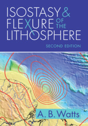
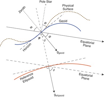
The techniques used by Condamine and Maupertuis involved the measurement of the distance between two points of known position. The positions were determined astronomically by measuring the angle of elevation, Φ, between the pole star (Polaris) and the horizon, as indicated by level bubbles on an astrolabe. Level bubbles follow a surface, known as an ‘equipotential surface’, along which no component of gravity exists. The equipotential surface, which coincides with Earth’s mean sea level, is known as the ‘geoid’, and so Φ is the angle between the pole star and the geoid. Because the direction of the pole star is normal to the equatorial plane, then it follows (Fig. 1.1) that Φ is also the angle between the normal to the geoid (i.e., the plumb-line direction) and the equatorial plane and, hence, the astronomical latitude at a point.
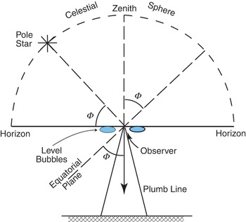
Figure 1.1 The determination of astronomical latitude, Φ, from observations of the pole star.
The distance between astronomical positions was determined by triangulation. In this technique, a network of triangles with vertices permanently marked on the Earth’s surface are set up so that they connect the astronomical positions. One of the astronomical positions is then chosen as one vertex on the first triangle. If the length of one side of the triangle and its included angles are accurately measured, then it is possible to determine the distance between each vertex of the triangle. By extending the network of triangles to include the second astronomical position (Fig. 1.2), it is possible to estimate the total distance between astronomical positions from an accurate measurement of a length in the first triangle (which may be quite short) and the angles between vertices of all the other triangles.
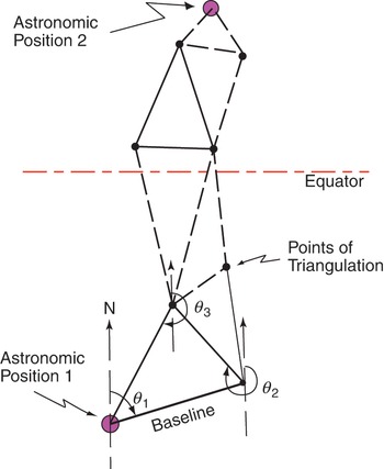
Figure 1.2 The measurement of the distance between two points by triangulation where astronomical latitude and longitude have been determined.
The length of the meridian degree measured by Condamine was, as it turned out, much smaller than that measured by Maupertuis (Table 1.1). Furthermore, the length of the meridian degree on the Arctic Circle was greater, by about 900 m, than the length determined previously near Paris; and the length near the equator was smaller, by a slightly larger amount. These results convinced Condamine and Maupertuis that the Earth was indeed flattened at the poles, as suggested by Newton. The flattening, fe, was estimated to be about 1/216.8 (Fig. 1.3). The measurements of Condamine and Maupertuis therefore solved the controversy of the overall shape of the Earth, although perhaps not quite in the way their sponsor, the Royal Court in Paris, had anticipated!
Table 1.1 Summary of measurements of the length of a degree meridian according to the surveys led by Condamine and Maupertuis
| Nearest Town/City | Approximate Latitude | Length of a Meridian Degree (ToiseFootnote *) | Difference from Paris (ToiseFootnote *) |
|---|---|---|---|
| Tornio, Finland | 66° (Arctic Circle) | 57,525 | +342 |
| Paris (L’observatoire de Paris) | 48° 50’ | 57,183 | 0 |
| Quito, Ecuador | 0° (Equator) | 56,753 | −430 |
* 1 Toise = 1.949 m.
Figure 1.3 The flattening of the Earth, fe, can be approximated by an ellipse with semi-major axis, a, and semi-minor axis, b.
One member of Condamine’s party though, Pierre Bouguer (1698–1758; Fig. 1.4), was not content, however, to let the matter rest there. Bouguer was puzzled by the consistency of the results because the measurements near the equator were obtained in the presence of much greater topographic relief than those near the Arctic Circle. He surmised (Reference BouguerBouguer, 1749) that the mass of the mountains in the vicinity of Quito was sufficiently large that it should have caused the local plumb line to be deflected by as much as 1′ 43″ from the vertical.Footnote 1 Such a deflection would introduce errors into the astronomical positions because the elevation of a distant star is measured on a table with level bubbles so that the measurement is made with respect to the local plumb-line direction (Fig. 1.1). The astronomical positions were apparently not in error, however, leading Bouguer to conclude that the attraction of the mountains in the vicinity of Quito ‘is much smaller than expected from the mass of matter represented in such mountains’.

A few years later, an Italian astronomer and mathematician with strong links to Croatia, Ruggero Giuseppe Boscovich (1711–87), provided an explanation of the problem that puzzled Bouguer. He said (Reference BoscovichBoscovich, 1755): ‘The mountains, I think, are to be explained chiefly as due to the thermal expansion of material in depth, whereby the rock layers near the surface are lifted up. This uplifting does not mean the inflow or addition of material at depth, the void within the mountain compensates for the overlying mass.’
This passage is the first to use the term ‘compensates’. Boscovich speculates that the mass excess of the mountain is compensated in some way by a mass deficiency at depth. Thus, the deflection of a plumb line near a mountain range may well be small, as Bouguer had suspected.
Boscovich, with broad interests beyond astronomy and mathematics, may, we speculate, have been influenced by a fellow Italian, the eminent scientist Luigi Ferdinando Marsigli (1658–1730). In 1728, 27 years prior to the appearance of Boscovich’s paper, Marsigli illustrated in a beautiful set of drawings the difference in elevation and thickness of ‘marine’ (oceanic) and ‘mountainous’ (continental) crust. His beautiful, hemispherical, water-coloured and pen-drawn cross sections show a juxtaposed mountain-peak height and seafloor depth that appear to be in some sort of isostatic balance with a thicker crust beneath the mountains than beneath the oceans (Reference Vai, Vai and CaldwellVai, 2006).
Little more appears to have been said on the matter for another 100 years. The statements made by Boscovich and the drawings of Marsigli on the compensation of mountains, as significant as they were, evidently had little impact on leading geologists of the time.
In the early 1800s geological thought in Europe was dominated by the contraction theory. According to this theory, the Earth’s surface features were thought to have been the consequence of a gradual cooling of the Earth following its formation. Mountains were considered to be regions that had not cooled as much as ocean regions. The theory had its origins in the work of Gottfried Wilhelm Baron von Leibnitz (1646–1716) and René Descartes (1596–1650). Baron Jean Baptiste Joseph Fourier (1768–1830) subsequently measured the temperature gradient at shallow depths in the Earth, concluding that it was in accord with the predictions of the contraction theory. Therefore, Boscovich’s statements on the thermal expansion of mountains may not have seemed all that inconsistent with the theory.
The eminent British geologist, Charles Lyell (1797–1875), was sceptical about the contraction theory. By 1833 he had completed his widely acclaimed book, Principles of Geology (Lyell, 1832–3), in which he proposed that the Earth’s surface is continually subject to periods of rest and change. He disagreed strongly with theories of catastrophes to explain geological events and with ideas forwarded by Leonce Elie de Beaumont (1798–1874) in France and Henry Thomas de la Beche (1796–1855) in England that geological processes, such as mountain building, were global events that occurred at similar times over widely separated regions. Lyell wrote: ‘It is preposterous to imagine that just because they had similar trends the Allegheny and Pyrhenees mountain ranges could have been formed by the same catastrophic event.’ Among Lyell’s many influential friends was John Herschel (1792–1871, Fig. 1.5). In a letter addressed to Lyell, Reference Herschel and BabbageHerschel (1836) pointed out that he disagreed with the contraction theory. In his opinion, the outermost layer or ‘crust’ of the Earth was in some form of dynamic equilibrium with its underlying substratum or ‘sea of lava’. He wrote ‘the whole (crust) [floated] on a sea of lava’. According to Herschel, if the crust was loaded, say by sediments, it would sink, thereby causing the underlying lava to flow out from beneath the load and into flanking regions (Fig. 1.6).
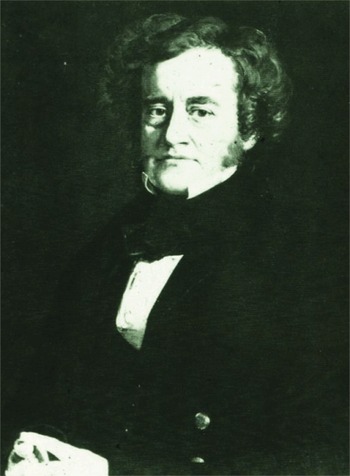
Figure 1.5 John Frederick William Herschel, the son of the astronomer William Herschel who discovered the planet Uranus.
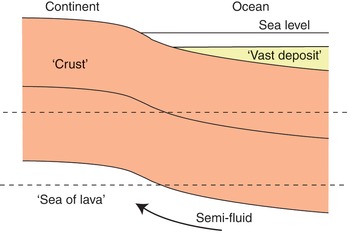
Figure 1.6 The adjustment of the crust to a ‘vast deposit’ by flow in the underlying ‘sea of lava’.
Herschel’s ideas on the equilibrium of the Earth’s crust might never have been published had it not been for Charles Babbage (1790–1871), the mathematician and inventor of the computer, who had also befriended Lyell. Babbage decided to include the letter that Lyell had received from Herschel in a treatise he was writing. The treatise was prepared by Babbage, on his own initiative, as a sequel to the eight volumes of the ‘Bridgewater Treatise’, which had just been published using proceeds from Lord Bridgewater’s estate. Babbage felt compelled to publish a ninth treatise because, in his opinion, a prejudice was emerging that the pursuit of science was unfavourable to religion. In a letter to Lyell, he pointed out that the ninth treatise would provide ‘an opportunity to illustrate some of the magnificent examples of creation’.
In the ninth treatise Babbage included some observations (Reference BabbageBabbage, 1847) he had made at the Temple of Serapis in Pozzuoli, Italy. Built towards the end of 200 AD, the temple had served as a spa (Fig. 1.7) for wealthy Romans. When Babbage visited the site in 1828, the temple’s three remaining columns showed a dark encrustation about 4 m above their base. Above the dark encrustation, 2.5 m of the column had been perforated in all directions by a marine boring animal (Modiola lithophaga). This observationFootnote 2 suggested to Babbage that the temple had undergone a period of subsidence, followed by one of uplift. He attributed these movements of the crust to the action of heat, because of the location of the temple near the historically active volcano of Vesuvius. Babbage considered that the heating caused the crust to expand and contract locally and that these movements were in some way accommodated by movement in the underlying fluid lava. Thus, Herschel and Babbage agreed that the crust accommodated loads by lateral flow in a weak underlying substratum. While Lyell supported this view, it was strongly opposed by the supporters of the contraction theory, who believed that the subsidence and uplift was the consequence of thermal contraction and expansion on a global scale.
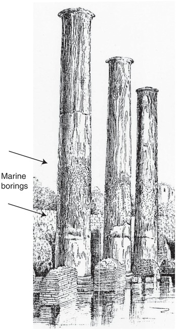
Figure 1.7 The Temple of Serapis in Pozzuoli, Italy. The borings in the Roman-built columns were used by Babbage to infer that the crust had undergone subsidence followed by uplift.
The ninth Bridgewater treatise was published in 1837, the same year that Charles Darwin (1809–1882) made a brief statement, to the Geological Society of London,Footnote 3 on some observations on the subsidence of ocean islands he had made during his circumnavigation of the world onboard HMS Beagle. Darwin, who was given a copy of Lyell’s book by Captain FitzRoy at the start of the voyage, recognised three types of ocean islands: volcanic, coral and combinations of the two. It was his view (Reference DarwinDarwin, 1842, p. 98, woodcut 4; p. 100, woodcut 5) that a submarine volcano would grow up on the seafloor to become a high island. Coral would grow in the shallow water fringing the volcano (e.g., as at Moorea in the Society Islands), and then as the volcano started to subside, the coral would attempt to keep pace and grow upwards, leaving a gap between a ‘barrier reef’ and the central volcanic island (e.g., as at Bora Bora in the Society Islands). Eventually, the island would sink below sea level and all that would remain is an atoll with a central lagoon (e.g., as at Aratika in the Tuamoto Islands). Darwin found direct evidence for subsidence at Santiago in the Cape Verde Islands where the volcano had ‘disturbed’ and ‘bent’ downwards a ‘bright white’ layer of limestone,Footnote 4 which Darwin supposed had been deposited horizontally and now underlay the volcano edifice (Reference DarwinDarwin, 1844, p. 9, woodcut No. 2). He went on to propose that either the volcano had been uplifted and then subsided or that it had never been uplifted, which implied that the volcano somehow maintained its elevation despite the subsidence. Interestingly, from the viewpoint of isostasy, Darwin favoured the latter hypothesis.
It is tempting to speculate that the observations of Herschel and Babbage and, especially, those of Darwin relating to subsidence and uplift had set the scene for the next major development in our understanding of the science of the equilibrium of Earth’s crust. However, it was not the geologists, but the geodesists who were to make the key observations that eventually led to the theory of isostasy.
1.3 The Deflection of the Vertical in India
The first measurements of the length of a meridian degree in the India sub-continent were carried out in 1840–59 by George Everest (1790–1866), who as Surveyor-General was charged with mapping the country. Everest’s measurement techniques differed from those of the earlier surveys of Condamine and Maupertuis, as he considered astronomical as well as geodetic positions. Geodetic positions were computed at the vertices of each triangle by assuming the position at one vertex of the first triangle was known and then using the equation for the Earth’s best-fitting reference ellipsoid to compute the other positions (Fig. 1.8). (Thus, instead of regarding the flattening of the Earth as an unknown, as the Condamine and Maupertuis parties had, Everest assumed it was by now well enough known to compute geodetic positions at points in between the astronomical positions.)
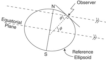
Figure 1.8 The determination of geodetic latitude, ϕ, from the theoretical formula for the Earth’s best-fit reference ellipsoid.
At points where both astronomical and geodetic positions are determined, it is possible to compare them. As Fig. 1.9 shows, astronomic and geodetic latitudes are referenced to a common surface: the equatorial plane. The astronomic position is defined as an angle between the equatorial plane and the local plumb-line direction, whereas the geodetic position is defined as an angle between the equatorial plane and the local normal to the Earth’s best-fitting ellipsoid. The plumb-line direction does not necessarily follow the local normal to the ellipsoid because of disturbing masses in the Earth. The amount that the plumb line is deflected from the local normal is known as the ‘deflection of the vertical’.
As part of his survey in India, Everest computed the geodetic position at a number of localities where he had already measured the astronomic position. He found that for two stations, Kaliana and Kalianpur, on the Ganges Plain to the south of the Himalaya, the latitude difference between them computed geodetically was 5.24″ smaller than that determined astronomically. Reference EverestEverest (1847) thought the discrepancy was unlikely to be in the astronomical position, which he considered to have been determined accurately, but in the geodetic position. He discussed the possibility the discrepancy was caused by the lateral gravitational attraction of the topography of the Himalaya (Everest, p. 179, 1st Hypothesis); but his preferred explanation was closure errors and an incorrect reference ellipsoid, which he then proceeded to ‘disperse’ throughout the triangulation surveys (Everest, p. 179, 2nd Hypothesis).
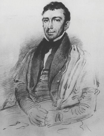
But a Caius College, Cambridge–educated mathematician, John Henry Pratt (1809–71: Fig. 1.10), who was Archdeacon of Calcutta at the time, disagreed with the so-called ‘process of dispersion’. He believed the discrepancy could be directly related to the disturbing effects on the plumb line of the nearby Himalaya. As Bouguer had previously pointed out, the gravitational attraction of nearby mountains could locally perturb the direction of the plumb line, thereby introducing an error into the astronomic positions, since these positions are used to calculate the deflection of the vertical. Indeed, the largest discrepancies measured by Everest and his assistants during the survey of India were between Kaliana and Kalianpur, and Kalianpur was within 200 km of one of the highest peaks in the Himalaya. It was therefore somewhat surprising Everest did not favour an explanation based on gravitational attraction of nearby topography, especially since he was well aware of its influence on the direction of the plumb line and astronomical observations from his earlier surveying experiences in the Cape Province, South Africa.Footnote 5

In a paper read before The Royal Society of London on December 7, 1854, Pratt presented the results of his calculations of the gravitational attraction due to the Himalaya and its hinterland at Kaliana and Kalianpur. He estimated the attraction by dividing the mountains up into ‘compartments’, computing the gravitational attraction of each compartment, and then summing the results. The problem was determining the topography of the Himalaya and its hinterland. Since the region was largely unexplored, Pratt had to rely on interviews with travellers who had returned from the area!
Consider an elementary mass
 at M and a unit mass at P. The gravitational force of attraction,
 , between the masses is given by Newton’s inverse square law:
 (1.1)
(1.1)
where G is the universal gravitational constant and d is the distance between the two masses. In the case that M and P are points on the surface of a spherical Earth, then it follows (Fig. 1.11) that the component of the attraction at a station P due to the elementary mass at M in the direction of gravity is given by

where

 (1.2)
(1.2)
Pratt used Eq. (1.2) to calculate the gravitational effect of the Himalaya at Kaliana and Kalianpur, and published the results in a 75-page paper (Reference PrattPratt, 1855). By subtracting the gravity anomaly on the ellipsoid from the gravity anomaly due to the mass excess of the mountains, he calculated a plumb line deflection of 15.885″, more than three times the observed value (Reference EverestEverest, 1847, Fig. 1.12). Pratt was satisfied, despite problems with not knowing the detailed topography of the Himalaya, that he had correctly computed the effect of the mountains at Kaliana and Kalianpur. He concluded his paper by stating that he did not understand the cause of the discrepancy and that the problem should be investigated further.
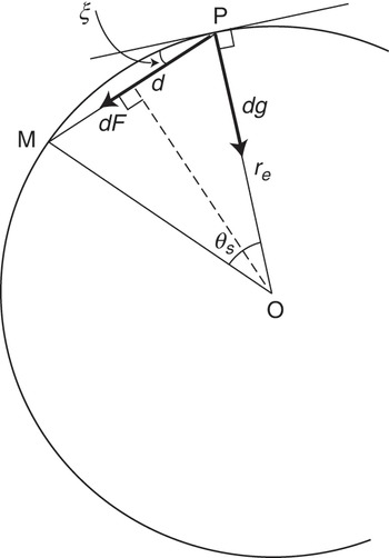
Figure 1.11 Pratt’s determination of the gravitational attraction, dg, at a station P due to a mass dm at M.
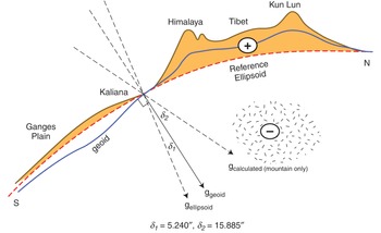
Figure 1.12 The deflection of the vertical at Kaliana, northern India. Deflection δ1 is the deflection determined by Everest from astronomic and geodetic observations. Deflection δ2 is the deflection calculated by Pratt due to the mass excess of the Himalaya, Tibet and Kun Lun above sea level. The shading schematically shows the mass deficiency that was inferred by Airy and, later, Pratt to underlie the mass excess.
1.4 Isostasy According to Airy
Shortly after Pratt’s paper, George Biddell Airy (1801–92; Fig. 1.13), the Astronomer Royal, presented a paper to the Royal Society in which he offered an explanation for the discrepancy. Unlike Pratt, Airy was not surprised by the discrepancy. Indeed, he thought it should have been anticipated.
Airy’s argument was based on his belief that the outer layers of the Earth consisted of a thin crust that overlay a fluid layer of greater density than the crust. He referred to the fluid layer as ‘lava’. Airy compared the state of the crust lying on the lava to timber blocks floating on water. He wrote (Reference AiryAiry, 1855, p. 103):
the state of the Earth’s crust lying upon the lava may be compared with perfect correctness to the state of a raft of timber floating upon water; in which, if we remark one log whose upper surface floats much higher than the upper surfaces of the others, we are certain that its lower surface lies deeper in the water than the lower surfaces of the others.
By using the analogy of icebergs, Airy suggested that a wide, flat-topped mountain or ‘tableland’ would be underlain by a less dense region, such that there would be a substitution of ‘light crust’ for ‘heavy lava’. The effect on the local direction of gravity, he viewed, would depend on two actions: the positive attraction of the elevated ‘tableland’ and the negative attraction of the light crust. He argued that the reduction in attraction of the light crust would be equal to the increase in attraction of the heavy mass above, so that the total effect on the local direction of gravity would be small. This argument, which he was able to make in a three-page-long paper, provided a simple explanation for the observations of Everest.
Airy was quite cautious in applying his model, pointing out that it may not be entirely appropriate to consider all features on the Earth’s surface as in a state of flotation. In the case of a tableland (e.g., Tibet), for example, Airy argued that it was unlikely to be supported in any way, other than by a lower-density crust that protruded into the underlying ‘lava’. He argued that ‘fissures’ or ‘breakages’ would form at the edges of the tableland (Fig. 1.14). In the case of narrow features, such as Mt. Schiehallion in Perthshire, Scotland- where the Rev. Maskelyne (1732–1811) had previously used the deviation of the plumb line to estimate the mean density of the Earth, Airy suggested that his model may not apply, implying that the crust might be sufficiently strong to support this feature without fissure or breakage.
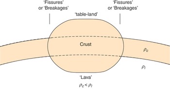
Figure 1.14 Airy’s hypothesis of a crust that ‘floats’ upon ‘lava’.
1.5 Isostasy According to Pratt
There is little doubt that Airy’s paper must have come as a surprise to Pratt. Pratt was a mathematician, and his approach to the problem was to carry out detailed, somewhat tedious calculations. Airy, on the other hand, approached the problem without mathematical reasoning, using simple physical concepts. Furthermore, there was a difference in the amount of work carried out; Pratt’s paper was 75 pages in length, while Airy’s contribution was only three pages!
In 1858, Pratt followed up on Airy’s suggestions on mass excess and deficit, proposing his own model for the equilibrium of the Earth’s outer layers. He criticised Airy’s model on three main grounds (Reference PrattPratt, 1859). First, the model was based on the assumption of a thin crust. Second, the model assumed that the crust was less dense than the underlying lava. Third, the model was not in accord with the prevailing contraction theory of the Earth. The first objection was based on a suggestion by a colleague of Pratt’s at Cambridge, Mr. Hopkins, that the Earth’s crust was at least 150 km thick. The second and third objections, however, were clearly a result of Pratt’s adherence to the contraction theory.
In 1864 and 1870 Pratt presented two further papers on the subject to the Royal Society. In particular, he expanded on his view, based on the contraction theory, that the depressions and elevations of the Earth’s surface were the product of thermal contraction and expansion (Reference PrattPratt, 1864; Reference Pratt1871). He stated that the ‘amount of matter in any vertical column drawn from the surface to a level surface below the crust is now and ever has been, approximately the same in every part of the Earth’. This statement implies (Fig. 1.15) that elevated regions were underlain by low-density rocks, whereas depressed regions were underlain by high-density rocks. Unlike Airy, however, Pratt did not speculate on what might cause different portions of the Earth’s outer layers to be colder or hotter than others. But he recognised these regions as providing the compensation for surface depressions and elevations, a term that had not been used since Boscovich’s study.
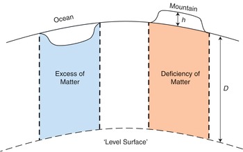
Figure 1.15 Pratt’s hypothesis that mountains are underlain by low-density regions while oceans are underlain by high-density regions. At some depth, referred to as the ‘level surface’, masses are equal.
Despite Pratt’s criticisms, Airy did not return to the discussion. The only occasion it seems was when Airy presented a lecture to the Cumberland Association for the Advancement of Literature and Science. A brief edited abstract of his lecture was published in Nature in 1878 (Anonymous, 1878). Apparently, Airy did not even refer to Pratt’s model in his lecture: instead, he simply repeated the model that he had outlined to The Royal Society in 1855.
Pratt’s contributions to isostasy were even more remarkable given that his colleague in Calcutta, Bishop Wilson, died in 1858 and so he had to take up an increasingly active role in the church. He was, by all accounts, a much admired archdeacon, and one of his greatest achievements was the establishment of funds to support the ‘Hill schools’ in the Himalaya and a missionary girl’s school in Calcutta (Reference BrownBrown, 1872). The latter survives, and it is certainly fitting that the Memorial School, Jura Girja, one of the oldest and best known of the missionary schools, continues to recognise Archdeacon Pratt as its founder.
1.6 Fisher and Dutton on Isostasy
It is curious that the scientific discussions between Airy and Pratt during the 1850s were not really taken up by other workers at the time. The next development was not until 1881, when the Rev. Osmond Fisher published his book entitled Physics of the Earth’s Crust (Reference FisherFisher, 1881). Described by some as the first textbook in geophysics, the book pays little attention to the controversy between Airy and Pratt. Instead, its main purpose seems to have been to develop the arguments against the contraction theory, which was continuing to dominate geological thought at the time.
Fisher, like Herschel and Airy and Pratt before him, had his own views. He argued the crust and underlying substratum as being in some form of equilibrium: with the lighter crust floating on the denser substratum. He went on, however, to make an important new statement about how this equilibrium might be achieved. In his words (Reference FisherFisher, 1881, pp. 275, 278): ‘the crust must be in a condition of approximate hydrostatical equilibrium, such that any considerable addition of load will cause any region to sink, or any considerable amount denuded off an area will cause it to rise. … the crust analogous to the case of a broken-up area of ice, refrozen and floating upon water’.
With these statements Fisher had captured the essence of what would later be called isostasy. According to Fisher, the crust obeyed Archimedes’ principle. The weight of a floating block of crust of thickness B and density ρblock that is floating in a fluid substratum of density ρfluid is then equal to the weight of the fluid displaced (Fig. 1.16):
 (1.3)
(1.3)
where b is the depth that the block is immersed in the fluid. Fisher used the analogy of a relatively light iceberg (
 ) that floats in denser seawater (
 ) to estimate that the part of a crustal block that would be immersed in the fluid substratum would be about 9/10 of its total thickness. Using Maskelyne’s preferred value of
 , this implies
 , a plausible result if, as was thought in Fisher’s time, the material beneath the crust consisted of lava.

The American army officer and geologist Clarence Edward Dutton (1841–1912, Fig. 1.17) was captivated by Fisher’s book, writing a complimentary review of it in 1882 (Reference DuttonDutton, 1882) when Dutton was at the United States Geological Survey (Reference OrmeOrme, 2007). Like Fisher, Dutton opposed the contraction theory, especially since it was based on vertical rather than horizontal movements and therefore offered no explanation for folding in mountain belts. In Dutton’s words (p. 127): ‘this hypothesis (interior contraction by secular cooling) is nothing but a delusion and a snare, and the quicker it is thrown aside and abandoned, the better it will be for geological science.’
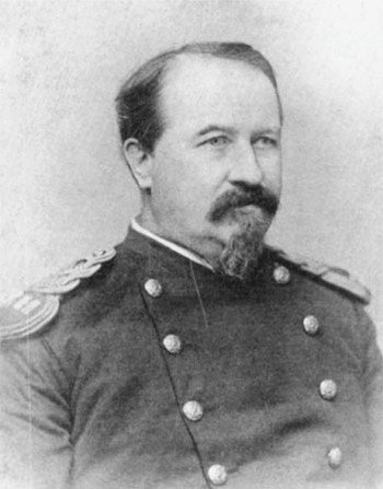
Figure 1.17 Captain Clarence Edward Dutton, Corps of Ordnance, US Army, who first developed what Reference BowieBowie (1927) later called the theory of isostasy.
Dutton’s review of Fisher’s book was noteworthy in another respect. The review contained the first reference to the term ‘isostacy’. In Dutton’s view, one of the ‘fundamental doctrines’ of Fisher’s book was the notion that the broader features of the Earth’s surface were simply those that were due to its flotation. This idea, he thought, should form an important part of any true theory of the Earth’s evolution. He wrote in a footnote (Reference DuttonDutton, 1882, p. 289): ‘In an unpublished paper I have used the terms isostatic and isostacy to express that condition of the terrestrial surface which follow from the flotation of the crust upon a liquid or highly plastic substratum … isobaric would have been a preferable term, but it is preoccupied in hypsometry’.
It took Dutton a further seven years, however, to publish the paper that he referred to in the footnote. In this subsequent paper, Reference DuttonDutton (1889) pointed out that if the Earth was composed of homogeneous matter, its equilibrium figure would be a true spheroid of revolution; but if some parts were denser or lighter than others, its normal figure would no longer be spheroidal. Where the lighter material accumulated, he argued, there would be a tendency to bulge, and where the denser matter accumulated there would be a tendency to depress the surface. He wrote (Reference DuttonDutton, 1889, p. 53): ‘For this condition of equilibrium of figure, to which gravitation tends to reduce a planetary body, irrespective of whether it is homogeneous or not, I propose the name isostasy.’ Thus, the term ‘isostasy’ (note that Dutton now spelled the word with an ‘s’ instead of a ‘c’) was born.
A major contribution of Dutton’s work was to point out the relevance of isostasy to geology. Isostasy, he argued, explained the subsidence of a large thickness of shallow-water sediments and the progressive uplifts of mountain belts. Subsidence and uplift were, in his view, a result of gravitation restoring isostasy to regions that were disturbed on the one hand by sedimentation and on the other by erosion. Dutton, however, also recognised limitations with isostasy, particularly in its inability to explain regional subsidence and uplift such as observed in submerged oceanic plateaus and uplifted mountain platforms that were once at sea level. Isostasy, as defined by Dutton, gives no explanation for such permanent changes of the level surface. On the contrary, he realised that isostasy is a working towards equilibrium that implies a certain degree of ‘protection’ of the crust against ‘massive lowering and raising’.
1.7 The Figure of the Earth and Isostasy
By the end of the nineteenth century, isostasy was still just an idea. It could not be proved by geological observations although, as Dutton pointed out, certain geological facts were in support of isostasy. The proof eventually came not from geology but from geodesy.
The science of geodesy may be considered as comprising two parts: geometrical geodesy and physical geodesy. In geometrical geodesy, triangulation techniques are used together with astronomical observations to determine information on the Earth’s shape. Physical geodesy, on the other hand, uses the Earth’s gravity field to determine its shape. The results of geometrical geodesy have been of immense practical importance in surveying on land.
The task of surveying the United States during the late 1890s was in the hands of the Coast and Geodetic Survey.Footnote 6 As a ‘frontier’ at this time, the western United States was experiencing booming land sales. It was important, therefore, that a network of monuments be established whose positions were accurately known. By the end of the nineteenth century, the Survey had carried out triangulation surveys along the Atlantic, Gulf and Pacific coasts. In addition, it had measured the astronomic positions at a large number of the triangulation stations. The triangulation of the country as a whole, however, was still not complete. When the triangulation surveys along the coasts were extended into the interior, it was found that significant gaps, overlaps and offsets occurred. These differences had to be eliminated if a national network of stations was to be established.
In 1899, John Fillmore Hayford (1868–1925) took charge of the Computing Division of the Survey and immediately set about the task of adjusting the different triangulation surveys. Early on in the work, Hayford realised that the source of error between the various surveys lay in the astronomical positions that were used to ‘fix’ the position of the monuments. The reason, he argued, was that these positions were referenced to the geoid, which, in turn, was influenced by the gravitational effect of the local terrain. He therefore corrected the astronomical positions for the gravitational effect of the local topography. The amount of work involved was enormous. This was because it was necessary to compute the effect of the topography above and below sea level, not only at the station, but also over an area within a radius of up to few hundred kilometres from the station point. In order to save time, Hayford constructed specially scaled templates for quickly reading topographic maps and employed a large number of workers (who he referred to in one publication as ‘computers’!) to carry out the tedious calculations.
Hayford found that by including the topographic correction he substantially improved the misfit between the different triangulation surveys. However, he found an even better fit if it was assumed that the topography was in some form of isostatic equilibrium. The question was which of the models of compensation that were available at the time should be utilised, Airy’s or Pratt’s?
For reasons that are not entirely clear, Hayford chose Pratt’s model rather than Airy’s. Perhaps Hayford, like Pratt, supported the contraction theory. Alternatively, it may have been the convenience of computation (Reference JeffreysJeffreys, 1926). In any event, Hayford’s choice was a popular one with his colleagues and it set a trend that was to last for more than three decades in which the ‘American school’ of geodesy preferred the Pratt model for their isostatic studies.
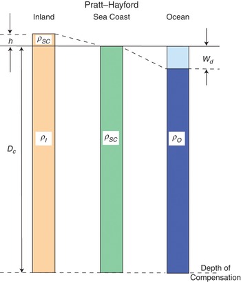
Unfortunately, the Pratt model was not in any form that could be used in geodetic computations. Hayford therefore parameterised the Pratt model. In setting up the model (Fig. 1.18), he made the following assumptions:
Isostatic compensation is uniform.
The compensating layer is located directly beneath a topographic feature and reaches to the depth of compensation, Dc, where equilibrium prevails.
The density of the crust above sea level is the same as the density of the crust at the coast.
The density of the crust below sea level varies laterally, being less under mountains than under oceans.
The depth of compensation is everywhere equal.
We can then write for the pressure PI at the base of a column of rock beneath a mountain,Footnote 7


and for the pressure Psc beneath a seacoast column,

Hence, for isostatic equilibrium we have

 (1.4)
(1.4)
The density of a column of rock beneath the ocean is then given by
 (1.5)
(1.5)
If we assume
 and
and
 (the value that Pratt later argued best minimised isostatic gravity anomalies), then Eq. (1.4) shows that the mean density underlying a 3-km-high elevated region is about 3 per cent less than under the seacoast. Similarly, with ρw = 1,030 kg m–3 we find from Eq. (1.5) that the density beneath a 5-km-deep ocean is about 3 per cent more.
The Pratt model was used by Hayford to correct the triangulation surveys of the entire United States. He found that the model successfully reduced the discrepancies between overlapping surveys (Reference HayfordHayford, 1909). Moreover, the model helped reduce the discrepancy between geodetic and astronomic positions. Hayford found, for example, that the discrepancy in the deflection of the vertical was on average reduced to about 10 per cent of what it would have been if no isostatic model had been used. With this success, it is little surprise that the Pratt model continued to be widely used not only in the United States, but also elsewhere, such as India (Reference BurrardBurrard, 1920) and Asia (Reference BowieBowie, 1926). Curiously, there were few attempts to use the model in Europe. As Sidney Gerald Burrard (1860–1943), the Surveyor-General of India, wrote (1920, p. 57): ‘The only countries so far that have calculated isostasy for their stations systematically are the United States and India. Europe has not touched the subject.’ When in 1924 the Europeans did address the issue, however, it was not Pratt’s model they turned to, but Airy’s!
During the 1920s most geodetic work in Europe was being carried out in Finland. In 1924, while at the Superior Technical School in Helsinki, Weikko A. Heiskanen (1895–1971) considered the different types of isostatic models available at that time, choosing the Airy model (Reference HeiskanenHeiskanen, 1931) ahead of Pratt’s for his isostatic calculations. Like Hayford before him, he had first to put the model in a more precise form. In doing this, he assumed the following (Fig. 1.19):
Isostatic compensation is uniform.
The crust as a whole is floating in a ‘sima-layer’ according to Archimedes’ principle.
The compensating masses lie directly beneath mountains and oceans.
The density of the crust is ρc everywhere and at every depth, and the density of the underlying ‘sima-layer’ is ρm everywhere and at every depth.
The thickness of the crust Tc at zero elevation is constant everywhere.
As in Hayford’s modification of the Pratt model, let us assume that the pressure at the base of a mountain column is equal to the pressure under a seacoast column. We can write for the pressure at the base of a column beneath the mountain, PI, that

and for a seacoast column,

Assuming isostatic equilibrium, we can then write that
 (1.6)
(1.6)
Equation (1.6) shows that beneath a 3-km-high mountain the crust would ‘project’ into the mantle by 12.7 km, assuming values of ρc and ρm of 2,670 and 3,300 kg m–3, respectively. This projection is called a root. The corresponding thinning of the crust beneath the oceans is called an anti-root.
By 1930, Finland had become one of the world’s leading countries for work in physical geodesy. A major focus was to use gravity anomalies to compute the shape of the Earth. This proved particularly useful in poorly surveyed land regions, and at sea where it was difficult to use triangulation techniques. The only problem was that in order to compute the Earth’s shape accurately it was necessary to know the gravity field everywhere. It was also important to use gravity anomalies that had been corrected for topography and its isostatic compensation (Reference LambertLambert, 1930).
Exactly why Heiskanen chose the Airy model for his geodetic work in preference to Pratt’s model is again not clear. In 1931, Heiskanen wrote (Reference Heiskanen1931, pp. 113–14): ‘the desire of helping isostatic research led W. Bowie during the Stockholm conference of the International Geodetic and Geophysical Union to suggest to me that I calculate complete isostatic tables based on Airy’s hypothesis.’
W. Bowie (1872–1940), who had joined the US Coast and Geodetic Service as an assistant to Hayford in 1909, was a firm supporter of the Pratt model. Only three years prior to the Stockholm meeting he had written (Reference BowieBowie, 1927, pp. 236–7): ‘the Airy theory is untenable …. The Pratt theory is the only one so far that is sound.’So, was Bowie being provocative in his suggestion to Heiskanen that he use the Airy model? Heiskanen later clarified the situation. In 1966, Heiskanen wrote (Reference Heiskanen and Hedgpeth1966, p. 777) that his reason for adopting the Airy model was because ‘from the geophysical point of view, the Pratt–Hayford assumption did not seem suitable’.
Because of Heiskanen’s work, the Airy model became well accepted throughout Europe. As a result, European and American geodesists were brought into a conflict with each other. The two schools of thought, however, were generally quite satisfied with the validity of isostasy. From their viewpoint, both the Pratt and the Airy models gave a satisfactory description of the density distribution of the outer layers of the Earth. A major question that remained was what was the geological significance, if any, of the different isostatic models?
1.8 Bowie’s Illustration of Isostasy
Although a geodesist, Bowie was concerned with how geologists viewed isostasy (Reference BowieBowie, 1927). He thought that geologists had difficulty in visualising isostasy, and so during his career he took several steps to try to explain its meaning. One of these, described in his book, involved setting up an experiment to demonstrate the simple physics that underlies the Airy and Pratt models of isostasy. The experiment was based on metal blocks that floated in an underlying fluid – materials that could be found in any physics laboratory.
Pratt isostasy is illustrated in Fig. 1.20a. Here, the blocks of different metals have been cast into prisms with the same cross-sectional area. Each prism has the same mass, but differs in length inversely with its density. If the prisms are placed in a vessel that is partly filled with mercury, each prism, because it has the same mass and cross-sectional area, displaces the same amount of mercury. The prisms exert the same pressure on the mercury, on which they rest, and so the lower surface of the prisms will be at the same level. We refer to the surface on which pressures are equal as the depth of compensation.

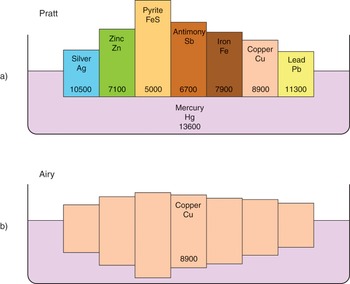
Figure 1.20 Bowie’s illustration of the (a) Pratt and (b) Airy models of isostasy using metal blocks floating in mercury.
Airy isostasy is illustrated in Fig. 1.20b. Here, the prisms are made up of just one metal and, hence, are of equal density. In this case, not only do the longer prisms stand higher than the shorter ones but also, they project downwards further into the underlying mercury.
The depth of compensation is more difficult to define for the Airy model than the Pratt model. One way is to consider it as the base of the prism that projects the greatest depth into the underlying fluid. This prism stands the highest in the fluid. All other prisms will stand shorter by an amount that is in proportion to the height of their bases above the base of the highest prism. The depth of the lower surface of the highest prism will therefore be a surface of constant pressure, like the depth of compensation in the Pratt model. The main difference with the Pratt model is that for all prisms, except the prism that projects the greatest depth, the pressure is made up of the weight of both the prism and the mercury.
A common feature of both the Pratt and Airy models is that individual prisms are separated from each other such that they are able to move up or down without constraint from their neighbours. Under these conditions, a prism that has mass added to it would move downward, while one that had mass removed from it would move upward. The material beneath the prisms would accommodate these movements by flowing, like a fluid. Therefore, if mass was removed from one prism and added to another, the fluid would move out from under the loaded prism to beneath the prism that had been unloaded.
Bowie pointed out that in the Earth’s crust there would, in fact, be great frictional and shearing resistance to any vertical movements arising from shifting of material from one region to another. However, he wrote (Reference BowieBowie, 1927, p. 25): ‘Since isostasy exists the crust must go up and down.’ The main questions that remained were the extent to which it went ‘up and down’ and whether or not there were instances where the strength of the crust might, in fact, resist these movements.
1.9 The Earth’s Gravity Field and Tests of Isostasy
The quantification of the Pratt model by Hayford and the Airy model by Heiskanen was of immense importance, not only for studies of the shape of the Earth, but also because they provided the means to test the extent of isostasy on a planetary scale. One test, for example, would be to calculate the gravitational effect of the models and compare it with measurements of the Earth’s gravity field.
The gravity field depends on the Earth’s shape and the distribution of masses within it. Isostasy involves the adjustment of the crust to the transfer of material across its surface. Therefore, departures of the gravity field from that which would be expected from models of the Earth’s topography and its compensation should indicate the scale to which isostatic equilibrium is achieved.
The first gravity measurements in the US were obtained during the 1890s by George Rockwell Putnam (1865–1953), an assistant to the director of the US Coast and Geodetic Survey. The measurements were based on observations of the period of a swinging pendulum, Tp, which depends inversely on the local value of the acceleration due to gravity, g. The relationship between g and Tp can be derived by consideration of the concept of a fictitious mathematical pendulum, which is a dimensionless mass hanging on a weightless thread. If the pendulum length is l, we can write
 (1.7)
(1.7)
In practice, several corrections have to be made to pendulum observations before they can be used to determine g. One of the most important is to correct for the movement of the stand that supports the pendulum. Other corrections that need to be applied are for temperature and pressure.
A practical difficulty was the long time that was required to make a gravity measurement. Putnam addressed this problem by using the new generation of light, portable pendulums, such as the quarter-second pendulum (Fig. 1.21). Unlike the early reversible pendulums which were of relatively long length, these relatively short-length pendulums were swung in a case in which the pressure had been reduced to one tenth of atmospheric using a portable air pump. By this means, the period of the more portable quarter-second pendulum’s swing could be increased and the time therefore that it took to make a gravity measurement reduced. By 1894, Putnam had measured gravity along a transect of the United States from the east to the west coast (Reference 561PutnamPutnam, 1895). In all, he acquired 26 measurements in 150 days. The highest measurement was obtained at Pike’s Peak, Colorado, at 4,312 m above sea level (the United States Geological Survey reported the height as 4,302 m in 2002), where it was found that the mean value of gravity after swinging three quarter-second pendulums twice was 9.78094 m s–2.
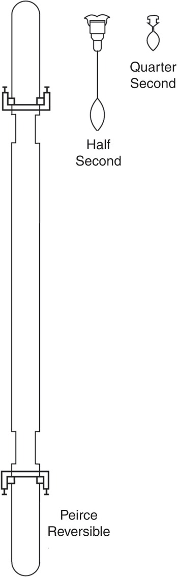
Figure 1.21 Comparison of the Peirce reversible pendulum that was swung in air with the half-second and quarter-second pendulums. The Peirce pendulum was used to make absolute gravity measurements at the Washington, DC gravity base station. The quarter-second pendulums, which were swung in a pressure-reduced case, were part of a portable measuring system used by George Rockwell Putnam to measure gravity in the United States during 1894. The complete apparatus consisted of three quarter-second pendulums that, together with their air pump, chronometer, and packing case, weighed 318 kg.
Putnam was not just concerned with the measurement of gravity. He was also interested in using gravity data to determine information about isostasy. But, first, it would be necessary to correct the observations for the shape and rotation of the Earth, the height of the station, and the mass that existed between a station and mean sea level.
To correct for the flattening of the Earth and its rotation, Putnam used a formula derived by the German geodesist Friedrich Robert Helmert that expressed the variation in gravity on an ellipsoid of revolution with a flattening, fe, of 1/293.5. The derivation of this formula is based on Clairaut’s first-order theorem and is obtained by solving Laplace’s equation to a spheroidal boundary. Clairaut’s theorem gives
 (1.8)
(1.8)
where


and gellipsoid is the value of gravity at some point on the ellipsoid, ge is the value of gravity at the equator, ϕ is the latitude, ω is the angular velocity of the Earth’s rotation, and a and b are the semi-major and semi-minor axes, respectively, that describe the ellipsoid that best fits the Earth’s flattening. Helmert obtained the following:
 (1.9)
(1.9)
where gellipsoid is in Gals (1 Gal = 1 m s–2 = 1,000 mGal). More widely used during the last century, however, have been the 1930 International Gravity Formula and the 1980 Geodetic Reference System. The 1930 formula was based on
 and a value of ge derived empirically from terrestrial gravity measurements based on the Potsdam worldwide gravity network and is given by Reference Heiskanen and Vening MeineszHeiskanen and Vening Meinesz (1958) as

The 1980 formula, on the other hand, was based on a satellite-derived fe = 1/298.257 and a value of ge corrected for the ~14 mGal difference between the older Potsdam and newer International Gravity Standardisation Net and is given, for example, by Reference Li and GötzeLi and Götze (2001) as

The variation of gellipsoid with ϕ is illustrated in Fig. 1.22 where it is compared to the maximum range of gravity values measured on Earth’s surface.

The correction for height of an observation station above mean sea level was computed using the ‘Faye correction’, later referred to as the free-air correction or FAC. This correction assumes no mass between the station and sea level. Then we can write

The plus sign represents an observation point above the geoid, and the minus sign a station below it. Now, we can also write

where re is the mean radius of the Earth, Me is the mass of the Earth and h is the height of the station above sea level. If we neglect higher-order terms in the expansion (i.e., h2/r2e, h3/r3e …), then we can write
 (1.10)
With
 and
and
 , this gives, neglecting high-order terms, FAC = 0.3080 mGal m–1. The difference in gravity on the geoid (which corresponds to mean sea level) and the reference ellipsoid is defined as the free-air anomaly, FAA.Footnote 8 We then have
 (1.11)
Finally, in order to correct for the effect of mass distributions between the station and the geoid, Putnam used an ingenious method of constructing rings around a station point and computing their effects using expressions derived from the gravity effect of a cylinder. We can write the following formula for the gravitational attraction of elementary mass dm acting on a unit load at a station S above the axis of a vertical cylinder (Fig. 1.23):

where d is the distance between S and dm. For the Cartesian co-ordinate system shown in Fig. 1.23,

The component of df in the direction of gravity, dg, is given by

It is more convenient to replace x, y by polar co-ordinates r, θ. We can then write

where ρ is the average density of the elemental mass. The gravity effect of a ring of the cylinder can be obtained by integrating the effect of an elemental mass over the radius and height of the ring. We then get


 (1.12)

This is the form of the equation used by Reference 561PutnamPutnam (1895, p. 44). So, given the height of a ring (e.g., above sea level), L, its inner radius, r1, and outer radius, r2, and density, ρ, it is possible to compute its gravity effect. The total correction was obtained by summing the contributions of individual ‘rings’ around a station. This correction is known as the Bouguer correction (BC).
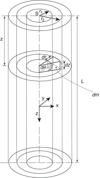
Figure 1.23 The calculation of the gravity effect of a vertical cylinder by consideration of the effect of a small, wedge-shaped element of mass.
For the special case that the topography extends at similar heights in all directions at a station, then

The Bouguer correction, BC, then becomes
 (1.13)
Equation (1.13) is known as the ‘Bouguer slab formula’ and is widely used in gravity anomaly reduction and interpretation. The formula assumes a planar surface, which is valid for the Bouguer reduction in small survey areas. In larger areas, account should be taken of Earth’s curvature. Reference QureshiQureshi (1976), for example, gives the formula for the gravitational attraction of a spherical cap of mass.
The Bouguer anomaly, BA, is the free-air anomaly corrected for the gravity effect of the masses above or below sea level. Hence,
 (1.14)
Putnam calculated the free-air and Bouguer anomaly at the 26 stations in the western United States where he had obtained gravity measurements (Table 1.2). He found that the Bouguer anomaly values over the mountainous regions of Colorado were strongly negative, which indicated to him that there was a significant deficit of mass beneath these regions. He went on to suggest that this was the deficiency of mass that compensates for the excess of mass of the elevated regions. What intrigued Putnam was that the deficit was largest at Gunnison (2,340 m) in the central part of the Rockies, and not at Pikes Peak, the most elevated station. He attributed this to the existence of an excess of gravity in the vicinity of Pikes Peak, pointing out that this was also visible in the free-air anomaly over the region.
Table 1.2 Summary of some of the measurements acquired by G. R. Putnam during the 1894–1895 trans-continental gravity survey of the western United States
| Station | Elevation (m) | Free-Air Anomaly (mGal) | Bouguer Anomaly (mGal) |
|---|---|---|---|
| Gunnison, CO | 2,340 | −7 | −263 |
| Pikes Peak, CO | 4,293 | 226 | −239 |
| Salt Lake City, Utah | 1,322 | −53 | −179 |
Even though Putnam’s work was based on only 26 stations, it was an important landmark in the development of the concept of isostasy. For example, he argued (Reference 561PutnamPutnam, 1895, p. 51) that ‘the results of this series would therefore seem to lead to the conclusion that general continental elevations are compensated by a mass deficiency of density in the matter below sea level, but that local topographical irregularities, whether elevations or depressions, are not completely compensated for, but are maintained by the partial rigidity of the earth’s crust.’ This is one of the earliest statements made concerning the spatial extent of isostasy in continental regions, and the first to hint isostatic equilibrium may not be complete everywhere.
By 1909, many gravity measurements had been obtained in other regions in the United States. To test the extent of isostasy more routinely at each station, Hayford devised a procedure similar to the one used earlier by Putnam. The main difference was that Hayford computed the gravity effect of isostatic compensation at each station using a model of isostasy, in his case Pratt. Another difference was that he divided the rings of a cylinder centred on each station into compartments (e.g., Fig. 1.24). It follows from the work of Putnam that the gravity effect of a compartment is given by
 (1.15)
where
 is the density of the rock mass above sea level, h is the height of the compartment above sea level, r1 is its inner radius, r2 its outer radius,
 the azimuth of one side of the compartment and
 the azimuth of the other side. The gravity effect of each ring (or ‘zone’ as Hayford defined them) can then be obtained by summing the effects of individual compartments which could have different heights.
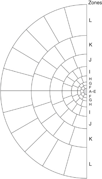
Figure 1.24 An example of one-half of a template used by John Fillmore Hayford to compute the gravitational effect of topography and its compensation at a gravity station. Each template would be drawn to a particular topographic map scale. The ‘zones’ are circles around a station, each of which is divided into compartments. The topography was averaged in each compartment and the gravity effect looked up in tables. Even with the tables, Hayford’s assistants took an average of 17 hours to calculate the topographic and isostatic corrections at an individual station.
The gravity effect of the compensation, or isostatic correction (IC), can also be computed from these parameters. Using the Pratt–Hayford scheme for land areas gives
 (1.16)
The anomaly that was obtained by subtracting the BC and the IC from the free-air gravity anomaly was defined by Hayford as ‘the new method anomaly’. We now know it as the ‘isostatic anomaly’. The isostatic anomaly is given by
 (1.17)
In 1909, Hayford presented the results of his isostatic anomaly calculations for 56 stations in the United States. He found that the isostatic anomaly was smaller than either the free-air or the Bouguer gravity anomaly. Since the isostatic anomaly incorporates corrections not only for the topography but also for the compensation, the magnitude of the anomaly provides some measure of the degree of compensation of a region: small-amplitude isostatic anomalies indicate that a geological feature is in some form of isostatic equilibrium, while large-amplitude anomalies indicate that a feature is either partially compensated or is uncompensated. Hayford argued that, since isostatic anomalies were generally small at all the stations, isostasy prevailed.
Hayford’s work in the United States triggered an investigation into the state of isostasy in other regions. Using similar gravity reduction procedures, Bowie and others demonstrated that isostatic anomalies were also small at stations in southern Canada, India, Europe, western Siberia and islands in the Pacific Ocean. Reference BowieBowie (1922, p. 49) wrote that ‘it seems safe to assert that the theory of isostasy has been proven and that it may now be spoken of as the isostatic principle’. And by 1924 Heiskanen had completed a preliminary set of tables that could be used to compute the isostatic correction based on the Airy model. It therefore became possible in the United States and elsewhere to compare the isostatic anomalies based on the Pratt and Airy models. As Table 1.3 shows, the Bouguer gravity anomalies for stations in the mountainous regions are significantly reduced using both models of isostasy. The Pratt–Hayford model is associated with the smallest anomalies at two of the stations, while the Airy–Heiskanen model is associated with the smallest anomalies at the other two stations. Thus, gravity provides a test of isostasy, although it did not permit the early isostasists to distinguish between the different models.
Table 1.3 Comparison of the isostatic anomaly computed using the Pratt–Hayford and Airy–Heiskanen models for representative stations in North America


Isostatic anomalies have proved of much value in determining the extent of isostatic equilibrium in a region. They also provide information on the depth of compensation in the Pratt model and the thickness of the crust at zero elevation in the Airy model. Reference Hayford and BowieHayford and Bowie (1912), for example, concluded that the best overall fit to gravity data from the United States was for a depth of compensation of 113.7 km. However, Reference HeiskanenHeiskanen (1931) preferred a depth in the range of 20–40 km. The reason for the difference in depths is that these investigators used different models of isostasy. In the Airy model, the compensation takes the form of a relatively large density contrast at shallow depth, while in the Pratt model it is in the form of a small contrast extending to greater depths. If individual stations rather than the average are considered, however, large variations in estimates of the depth of compensation occur (e.g., Table 1.4).
Table 1.4 Sensitivity in the Pratt–Hayford model to variations in the depth of compensation and in the Airy–Heiskanen model to variations in the thickness of the crust at zero elevation for a representative station in North America and Europe, respectively
| Pratt–Hayford: Pikes Peak, Colorado, USA | |
|---|---|
| Depth of Compensation (km) | Pratt–Hayford Isostatic Anomaly (mGal) |
| 42.6 | −204 |
| 85.3 | +57 |
| 127.9 | +32 |
| Airy-Heiskanen: Sonnblick, Alps, Austria | |
| Thickness of crust at zero elevation (km) | Airy–Heiskanen isostatic anomaly (mGal) |
| 20 | −10 |
| 30 | −24 |
| 40 | −35 |
The pioneering studies of Hayford, Bowie and Heiskanen were followed by several studies which used the isostatic gravity anomaly to assess the state of equilibrium of the Earth’s crust and mantle. Early studies using either profiles (e.g., Fig. 1.25) or maps (e.g., Fig. 1.26) were based on the Pratt–Hayford scheme. Later, the Airy–Heiskanen scheme was used.
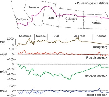
Figure 1.25 The first continuous trans-continental gravity anomaly and topography profile of the western United States. The purple solid line shows the profile, and the filled circles show the stations previously occupied by Putnam.
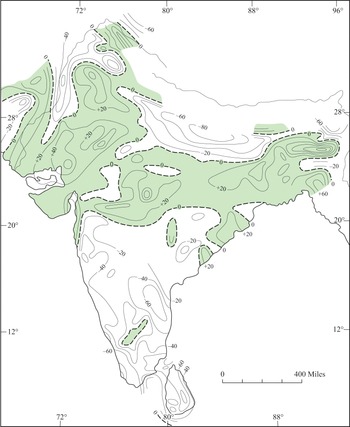
Figure 1.26 Isostatic gravity anomaly map of India based on the Pratt–Hayford hypothesis with Dc = 113.7 km. Green-shaded regions highlight positive isostatic anomalies. India has been considered the birthplace of isostasy because many of the early geodetic surveys were carried out there. Northern India, however, is associated with large-amplitude isostatic anomalies indicating a region out of isostatic equilibrium at least with regard to the Pratt model.
But, as pointed out earlier, gravity data were not able to distinguish between the two models of isostasy. The Pratt–Hayford model had certainly been used more widely than the Airy–Heiskanen model. However, as Jeffreys wrote in 1926 (p. 169): ‘Convenience of computation, and perhaps tradition, rather than any physical probability, have been the chief reasons for the attention given to Pratt’s hypothesis, and the lack of it to Airy’s.’ While there was therefore disagreement among the geodesists about the type of model to use in isostatic anomaly reductions, it was clear they thought that isostasy was an important doctrine that needed to be considered in geology. The problem was convincing the geologists. During the 1930s, for example, they appear to have been quite confused about the different models of isostasy and what information they implied, if any, about geological processes.
1.10 Isostasy and Geological Thought
The tests of isostasy that were carried out using gravity data convinced the geodesists that on the scales of continental masses, if not on the scales of mountain peaks and valleys, isostasy was operative. For example, Heiskanen wrote in 1931 (p. 111): ‘isostasy is no longer a hypothesis but a principle positively verified, which must be taken into consideration in geological investigations’.
But geological thought during the early 1900s continued to be perplexed by isostasy. As Reference GreeneGreene (1982) points out in Geology in the Nineteenth Century, the renowned Austrian geologist, Eduard Suess (1831–1914), declared himself a ‘heretic in all regarding isostasy’. The American geologist Reference ChamberlinRollin Thomas Chamberlin (1931, p. 1) summarised the situation as follows: ‘various geological observations and deductions, which the geologist regards as established facts, seem inconsistent with the isostatic theory as now applied by its leading advocates’. Chamberlin had little doubt about who to blame for the confusion (pp. 1–2): ‘To the geologist the recognised geologic facts, which he can understand and appreciate, are vastly more convincing than mathematical interpretations based upon assumptions, some of which he does not understand, and others of which seem to him clearly at variance with actual earth conditions.’ The principal problem was that the models used by the advocates of isostasy were static. Although the models enabled geodesists to calculate the disturbing effects on the gravity field of topography and its compensation, they provided little information on the origin of individual geological features. The geologists, on the other hand, based their work on careful field observations. By and large they were satisfied that they understood the processes that were responsible for the origin of the Earth’s surface features and they did not find it necessary to take isostasy into account.
The following facts, for example, seemed to Reference ChamberlinChamberlin (1931) to contradict the theory of isostasy:
The substantial amounts of shortening observed in mountain ranges could not be explained by simple vertical isostatic movements.
Isostatic models could not explain the existence of peneplane surfaces without requiring large amounts of erosion.
The substantial amounts of sediments in geosynclines could not be explained by isostatic processes alone, and so other factors must be operative.
The pattern of rebound of the continents following melting of the Pleistocene ice sheets did not follow the pattern of the ice load very closely.
Also puzzling to Reference ChamberlinChamberlin (1931) were the large variations in the depth of compensation that were required by Hayford and Bowie to minimise isostatic anomalies. Chamberlin questioned whether the depth of compensation was a physical entity. The query was understandable. All isostatic models tend to an equilibrium state. In an Airy model, the depth of compensation varies such that if crust is removed or added to, say by erosion or sedimentation, then isostatic equilibrium will be restored as the uniform density crust responds by thinning or thickening. But in a Pratt model, the depth of compensation is fixed and it is not immediately obvious exactly how equilibrium would be restored following a disturbance. In Chamberlin’s view, geological processes were complex, and he saw no reason why the process responsible for compensation of the Earth’s surface features should not be likewise.
Chamberlin’s views were shared by a number of other geologists at the time, notably Reference ShepardShepard (1923), Reference King-Hubbert and MeltonKing-Hubbert and Melton (1930) and Reference de Lyndonde Lyndon (1932). Reference ShepardShepard (1923, p. 208), for example, wrote: ‘In spite of the apparently indisputable evidence that the earth’s crust is in almost perfect isostatic adjustment, geologists have been slow to accept the theory of isostasy.’ He pointed out the difficulties of explaining the peneplanation of mountain ranges and their subsequent uplift in terms of isostatic models. Shepard attempted to explain these difficulties, however, by introducing other forces, such as lateral compression and uplift associated with volcanism. Reference King-Hubbert and MeltonKing-Hubbert and Melton (1930, p. 695), on the other hand, were not as condescending as Shepard. They wrote that ‘the theory of isostasy must, for the present, be regarded as resting upon a not too secure foundation and is hardly trustworthy for use as a major premise in present discussions of Earth problems’.
The other difficulty, raised by Reference de Lyndonde Lyndon (1932), concerned structural styles of mountain belts. He argued that the most striking features of the Uinta mountains (Colorado Rockies) were the over-turned anticlines and low-angle thrust faults which together proved that compression, not isostasy, was responsible for orogeny. The principle of isostasy should be considered in his view, but it was a minor, not a major contributor to Earth’s topography.
We learn from these discussions that despite the usefulness of isostasy to the geodesists, the concept remained a difficult one for the geologists to accept. Geologists such as Chamberlin recognised that isostasy was rooted in careful physical measurements and that it was supported by simple physical reasoning. But they were disappointed that despite all the hard work that Hayford, Bowie, Heiskanen and other geodesists had put in to quantify the Airy and Pratt models, the concept of isostasy could not be of more use in the solution of geological problems.
Not all geologists shared this disappointment. As Harry Fielding Reid, a contemporary of Bowie and Chamberlin, cautioned (Reference Bowie1922, p. 317): ‘Geologists often ask too much of the principle of isostasy. When they find that it will not explain all earth movements, they think it is not a true principle.’
1.11 Nature’s Great Isostatic Experiment
A few years after Chamberlin’s paper was published, Reginald Aldworth Daly (1871–1957), a Canadian geologist, published The Changing World of the Ice Age. In the book Reference DalyDaly (1934) describes the pattern of uplift and subsidence that followed loading of the North America and Fennoscandia crust by the great Pleistocene ice sheets. These patterns provide important information on the physical nature of the crust and its underlying mantle.
About 18 ka, a large portion of the Northern Hemisphere was covered by thick ice sheets, the largest of which were centred on Hudson Bay in Canada and on Sweden. There is evidence that the ice sheets were on the crust for a sufficiently long time that a state of isostatic equilibrium prevailed. Then, about 12.5 ka, the ice sheets began to melt. The melting upset the equilibrium, releasing large amounts of water into the surrounding oceans. The adjustment of the crust and upper mantle to shifts in ice and water loads is the subject of glacial isostasy.
The history of glacial-isostatic movements is recorded in raised (Fig. 1.27) and submerged (Fig. 1.28) beaches. By dating shells in the beach deposits using radio-carbon techniques it is possible to reconstruct the uplift and subsidence history of a region that has undergone a glaciation or de-glaciation event. Figure 1.29 shows, for example, the movements of a 6-ka surface that, prior to the melting event, was a horizontal surface at or near sea level. The figure shows that those regions that were loaded by the ice sheet are rising, while peripheral areas are sinking.
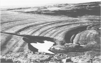
Figure 1.27 A view to the south of Richmond Gulf (Hudson Bay, Canada) showing the lichen-covered raised beaches.

Figure 1.28 A drowned river valley or ‘ria’ along the south-west coast of England.
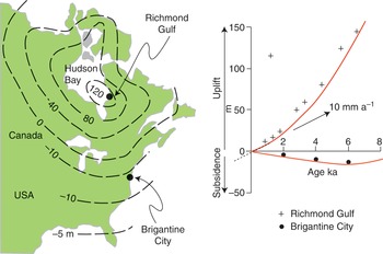
Figure 1.29 The pattern of glacio-isostatic rebound that followed the retreat of the Laurentide ice sheet. The graph shows the uplift measured at Richmond Gulf and the subsidence measured at Brigantine City (New Jersey, USA).
Daly, who had built on the earlier contributions of Thomas Jamieson and Nathaniel Shaler (Reference WolfWolf, 1993), examined the pattern of subsidence and uplift around the large Pleistocene ice sheets and concluded that they sank for two main reasons: elasticity and plasticity. He argued that the crust and upper mantle would respond to the weight of an ice sheet as an elastic material, such that if the ice load were removed through melting, then the crust and upper mantle would rebound elastically. If, however, the ice was on the crust long enough, then there would be flow such that the stronger crust would be ‘basined’ by the weaker underlying mantle. On melting, the crust would initially respond elastically, followed by a slow response as material in the mantle flowed back from flanking regions towards the loaded region.
In Daly’s view, the areas peripheral to an ice sheet were critical to understanding the mechanisms of adjustment. He believed, for example, that material in the mantle would flow out from beneath the load and into flanking regions. This pattern of flow would up-arch the strong crust in flanking regions, producing a peripheral bulge. On melting, the bulges would collapse, forming troughs adjacent to the uplift area (Fig. 1.30).
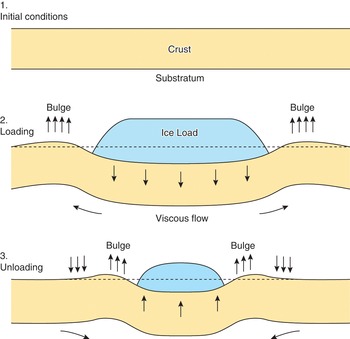
Figure 1.30 The ‘viscous bulge’ hypothesis to explain the pattern of uplift and subsidence of a deglaciated region.
Unfortunately, Daly was unable to corroborate these views in observed subsidence and uplift data. He therefore proposed a hypothesis, known as the ‘punching hypothesis’, which he thought better explains the observations. According to this hypothesis, ice sheets are large enough loads that they ‘indent’ the strong crust, setting up vertical shear stresses in the mantle that underlies the ice sheet. Eventually, mantle materials respond to these stresses by flowing. Because the whole mantle supports the ice sheet, at least momentarily, then on melting the whole mantle flows. A consequence of the punching hypothesis is that upon loading the flanking areas are dragged down but are eventually uplifted, whereas upon unloading the flanking areas are uplifted, then they subside.
A strong crust, as Haskell had earlier pointed out, is not actually required to explain the observed uplift and subsidence patterns. He developed a formula, based on the motion of a viscous fluid under a surface load (Reference HaskellHaskell, 1935), in which the time, t, to reach full (i.e., asymptotic) isostatic compensation is given by (Reference HaskellHaskell, 1937, eq. 5)
 (1.18)
where g is gravity, w is one-half width of a surface load, and η and ρ are the viscosity and density of the fluid respectively. Substituting Haskell’s preferred values of
 ,
,
 ,
,
 and
and
 into Eq. (1.18) yields a viscosity, required to explain the rise of the Fennoscandia area after melting of the ice, of ~8.35 × 10²⁰ Pa s. Therefore, flow in the mantle occurs naturally, and a strong crust is not required to explain observations. Haskell favoured Daly’s punching hypothesis, however, pointing out that the only way to produce the bulges would be to restrict the flow to a narrow, viscous channel beneath the region of the load.
An important feature of Daly’s hypothesis is that it involves some form of flow in the mantle that underlies the crust. As such, the hypothesis is in accord with isostasy. But isostasy as envisaged by Pratt and Airy is based on two fundamental assumptions:
that features on the Earth’s surface – no matter how small – are compensated for either by changes in crustal thickness or by lateral changes in density of the crust and mantle.
that the crust is ‘floating’ in a state of hydrostatic equilibrium with its surroundings, such that the mantle that underlies the crust has little or no strength.
The first assumption cannot be easily tested using the pattern of isostatic adjustments in North America and Fennoscandia. The reason for this is that the ice sheets that loaded these regions were so large that they caused significant yielding of the crust, largely uninhibited by its physical properties. Only perhaps in localised regions was the mass of the ice sheet sufficiently small not to cause yielding. Since these loads, both large and small, have largely disappeared, it is not possible to examine what relationship existed, if any, between the size of the ice sheet and the degree of yielding of the underlying crust.
Daly was, however, able to test the second assumption. His approach (Reference DalyDaly, 1939) was to use the information that was present in the gravity anomaly concerning the stresses that existed in the Earth’s outermost layers. He found, for example, that the former Fennoscandia ice sheet is associated with a free-air gravity anomaly low of about –20 mGal. Daly used the amplitude of the gravity anomaly as a measure of the compensation and hence the amount of ice that had originally been added to the crust. He found, using the Bouguer slab formula, that the equivalent height of an ice load of density 917 kg m–3 is 520 m.
Once the load had been estimated, Daly was able to apply the theory of George Howard Darwin, the son of Charles Darwin, for the deformation of an elastic half-space to calculate the maximum stress difference required to support that load (Reference DarwinDarwin, 1908). Darwin showed that for a periodic load of the form

the stress-difference at a depth z is given by
 (1.19)
where λw is the wavelength of the load. The maximum stress difference, σmax, is given by

which occurs at

The diameter of the negative free-air gravity anomaly over Fennoscandia is approximately 1,500 km, which corresponds to a wavelength of ~2 × 1,500 = 3,000 km. With values of
 ,
,
 and
and
 in Eq. (1.19), we get for the maximum stress difference,
 at a depth
 . The stress difference at 113.7 km, the depth of compensation according to the proponents of the Pratt model does not exceed 0.7 MPa. Thus, in the view of Daly, the assumption of a mantle with little or no strength, as suggested by the isostatists, was fully justified.
The gravity anomaly over a glaciated region is useful in one other regard, that of estimating the time that it would take for the deep flow to come to an end. Over the Laurentide ice sheet, for example, there is a close correlation (Reference WalcottWalcott, 1970c) between the free-air gravity anomaly and topography on the scale of a 1° × 1° ‘square’ (Fig. 1.31). Assuming this anomaly is due to warping of the crust by the ice sheet, then it is possible to calculate how far the depressed region must rise for the free-air anomaly to vanish. The equation we use is (e.g., Case 3, Fig. 1.32)
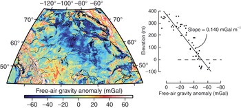
Figure 1.31 The free-air gravity anomaly over Canada and the northern United States and its relationship to the topography. The map is a downsampled 10 × 10 minute grid derived from the combined satellite and terrestrial gravity field grid (V31.1) of Reference Sandwell, Harper, Tozer and SmithSandwell et al. (2019). The gravity-topography slope plot is reproduced with permission from fig. 4 of Reference WalcottWalcott (1970c).
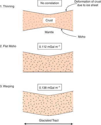
Figure 1.32 Expected correlation between free-air gravity anomaly and topography for different models of crustal structure. Note how close the calculated correlation between gravity and topography for the warping model is to the observed correlation in Fig. 1.31.


 (1.20)
With
 and
and
 , Eq. (1.20) yields y = 360 m. Therefore, the Hudson Bay region of Canada has a further 360 m to rise before equilibrium is re-established. At the 10 mm a–1 uplift rate that is observed today (Fig. 1.29) this will take some 30–40 ka, which is about a factor of two longer than that calculated earlier by Reference HaskellHaskell (1937).
Thus, the study of glacial isostatic adjustment has provided two important pieces of information on isostasy: one concerns the magnitude of the stresses that are supported by the mantle, and the other the timescales over which the phenomenon of isostatic adjustment occurs.
1.12 Success of the Airy and Pratt Models of Isostasy in Explaining Crustal Structure
Despite the studies of Daly and Haskell, most geologists in the late 1930s still paid little attention to isostasy. Perhaps they thought the spatial scales of glacial-isostatic adjustment were too large to be of interest to geological processes such as erosion and sedimentation which generally occur over much narrower tracts. Alternately, they thought that the timescales of glacial-isostatic processes were too short to be of interest to the long timescales of geological processes.
One exception was the Scottish-born American geologist Andrew Cowper Lawson (1861–1952), who had long championed the concept of isostasy. He published (Reference LawsonLawson, 1938, Reference Lawson1942) the first of several articles on the response of the crust and upper mantle to sediment loads in large river deltas. He showed, contrary to the opinions of Chamberlin, that substantial thickness of sediments could accumulate at a river delta simply by the isostatic adjustment to sedimentary loads.
The main ‘users’ of isostasy during the 1930s, however, continued to be geodesists. In Europe, efforts were being focused on determining the patterns of uplift in glaciated regions more precisely using geodetic techniques. In the United States, on the other hand, a new initiative was begun to use seismic techniques to determine the structure of the crust and upper mantle – one which was to have an immediate impact on isostasy.
Until the early 1950s, the gravity field had provided the principal means with which to test isostasy. But it soon became clear that gravity, due to its fundamental non-uniqueness, was limited in its ability to distinguish between the different isostatic models. Furthermore, the ‘best-fit’ depths of compensation determined by isostasists were strongly model dependent. Even though isostatic anomalies could be significantly reduced by changing the depth of compensation, the depths varied substantially according to whether the Airy or Pratt models were used.
A more satisfactory test of isostasy is seismic data on the structure of the crust and upper mantle. The Pratt and Airy models, for example, imply quite different crustal and mantle structure beneath an elevated mountain and a deep ocean basin. The Airy model predicts that these features would be compensated by changes in the thickness of a uniform-density crust, whereas the Pratt model predicts that they will be compensated by lateral changes in the density of the crust and mantle. The result is that the two models imply quite different depths of compensation. Isostatic gravity anomalies in the United States suggest, for example, a depth of compensation of about 40 km if an Airy model is used or a depth of 113.7 km for a Pratt model.
Following World War II, George P. Woollard (1908–79) and Maurice Ewing (1906–74) began an extensive program of seismic refraction measurements using explosive sources and geophones or hydrophones onshore and offshore the United States. The main result of these studies was to show that the crust is generally thickest beneath the continents and thinnest beneath the ocean basins. Figure 1.33 shows, for example, a compilation of the crustal thickness along a profile extending from Hawaii in the west, across the continental United States, to offshore France and Portugal in the east. The profile provides striking evidence that changes in topography are accompanied by changes in crustal thickness and, hence, that the Airy model provides a better description in general of the crustal structure than the Pratt model does.
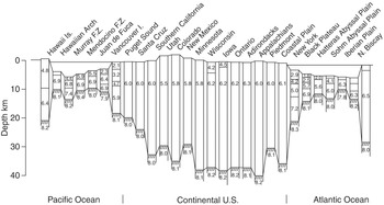
Figure 1.33 Seismic refraction profile of the crust and upper mantle structure from Hawaii Island in the west, across the mainland United States, to offshore France and Portugal. The profile shows striking support for the Airy–Heiskanen model of isostasy with mountains underlain by thick crust and oceans underlain by thin crust. The numbers in the columns are P wave velocities in km s–1.
It was clear from the earliest seismic measurements, however, that the relationship between topography and crustal thickness was not a simple one. The continental crust, for example, is actually thinnest in the western United States where the elevation is greatest, and thickest in the eastern United States where the elevation is smallest. Furthermore, in some oceanic regions, there are large lateral variations in crustal velocities that would not be predicted by the Airy model.
To better understand the departures from Airy isostasy, Reference Worzel and ShurbetWorzel and Shurbet (1965) used gravity anomaly and seismic refraction data to construct a so-called ‘standard’ oceanic and continental column. The continental column includes adjustments for the elevation above sea level and variations in the depth of the interface between crust and mantle. The ocean column was constructed in a similar way except there was no elevation correction applied. Figure 1.34 shows the standard columns that they adopted. Both columns are in balance with each other such that the free-air gravity anomaly over them would average to zero.
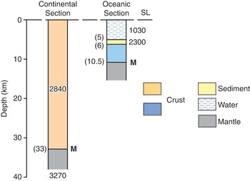
Figure 1.34 ‘Standard’ columns of the continental and oceanic crust. Unbracketed numbers are densities in kg m–3 and bracketed numbers are depths below sea level (SL) in kilometres.
The standard columns (Reference Worzel and ShurbetWorzel and Shurbet, 1965) have been widely used to test the state of isostasy at particular geological features. One example is shown in Fig. 1.35. The figure shows a compilation of the seismically constrained crustal structure across the margin offshore eastern Canada (Reference Keen, Keen, Barrett and HefflerKeen et al., 1975). The dashed line in the figures is the depth to the M-discontinuity in the transition zone as predicted assuming the Worzel and Shurbet standard column and the Airy model of isostasy. The figure shows a reasonably close fit between the seismic structure and the predictions of the Airy model, although there are departures in detail.
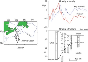
Figure 1.35 Gravity anomalies and crustal structure at the transition between oceanic and continental crust at the continental margin offshore Nova Scotia, Canada. The predicted Moho based on an Airy–Heiskanen model of isostasy is shown as a dashed line.
It would therefore appear from these discussions that seismology provides overwhelming support for isostasy. The crust is indeed lighter than the mantle that it overlies and, in this sense, is in a state of flotation. The question that remains is the ‘architecture’ of the crust. Is it characterised by lateral density changes in a crust of uniform thickness as predicted by a Pratt model or by changes in the thickness of a uniform-density crust as suggested by Airy? The evidence from seismic refraction data seems to favour the Airy model. However, as we will see in later chapters, the Pratt model, as well as other models, still have considerable merit.
1.13 Bloom’s Test of Isostasy
In 1967, A. Bloom (1928–) extended the earlier work of Daly and others on glacial isostasy by considering the effects that the transfer of water from the ocean to the ice sheets and the release of water from the ice sheet to the oceans would have on the isostatic balance of the stable part of the Earth’s crust (Reference BloomBloom, 1967). By examining the heights of former shorelines, he was able to test the concept of isostasy; in particular, to test the timescales at which isostatic adjustments might take place.
Bloom considered a simple model (Fig. 1.36) of a stable continent with a gently sloping shelf juxtaposed to an ocean basin. Initially, the shoreline is in equilibrium such that a notch will be cut at some position, say S1. If sea level then falls by h, a second notch will be cut at a point lower down on the shelf slope. The second notch will not necessarily be h below S1, however, because the ocean basin adjusts to the removal of water by uplift. The uplift causes water to spill over from the ocean basin and re-flood the shelf. Where the second notch is cut depends on how fast the crust adjusts to the removal of the water load. For example, if the adjustment is slow, then a notch will be cut first at S2, which is a height h below S1, and then at S3, which is a height y above S2. In the case of a fast adjustment, the sea level surface will proceed directly to S3 and there will be no intermediate notch cut at S2.

The heights between the old and new shorelines can be calculated by assuming that a column in the ocean is in local isostatic balance before and after unloading. Following Fig. 1.37, we then have

 (1.21)
Equation (1.21) shows that if sea level fell by an amount
 , the ocean basin will rise due to unloading by an amount
 , assuming
 and
and
 . The height between the shorelines and where a notch is cut will depend on how fast isostasy proceeds. If the uplift proceeds more slowly than the removal of water, then the distance between the upper and lower notches will be 108 m. If, however, the uplift proceeds rapidly, then the height between the shorelines is reduced to
 .
.

The height that sea level appears to an observer on the continent is called the freeboard. We see from Fig. 1.37 that the freeboard, f, associated with a sea level fall is given by

Usually, during glacial and inter-glacials a sea level fall is followed by a rise. A rise following the fall in the simple model in Fig. 1.37, for example, will cause the shoreline to move to a point above S3. If the rise is similar in magnitude to the fall and isostasy proceeds slowly enough, then the shoreline will move first to S4 where it might cut a notch. If, however, isostasy is fast, then the shoreline will move directly to S1 and there will be no intermediate notch at S4.
These considerations suggest that the height between the upper and lower shorelines following a sea level fall and rise will depend on how rapidly isostasy proceeds in relation to the time that it takes for the water to withdraw from and flood onto the shelf. In the case of a 108 m rise in sea level, the height between the shorelines will be 108 m for slow isostasy and 108 – 33 = 75 m for fast isostasy.
Sea level changes due to changes in ice volume will be recorded not only on the gently sloping shelves of the continents, but also on the steep slopes of oceanic islands. Oceanic islands are attached, however, to the oceanic crust, and so they respond directly. During a sea level fall and rise, for example, ocean islands rise and fall with the underlying ocean basin so that there will be no intermediate shorelines S3 and S4. Thus, ocean islands provide only limited information on how fast or slow isostasy proceeds. However, the height between the preserved shorelines on oceanic islands corresponds to S1 and S2 and therefore they have the greatest potential to determine the actual sea level change.
These considerations suggest that, if the isostatic model assumed by Bloom is correct, the height of continental shorelines should provide information on the rate of isostatic adjustment.
We compare in Table 1.5 the sea level rise that followed the last major glaciations as they are observed on oceanic islands and continents. The table shows that the sea level rise as observed on oceanic islands is significantly higher than that observed on the continents. This suggests that isostatic adjustment has been relatively fast, since otherwise the heights between shorelines on the continents would have been much higher. This is confirmed in the table, where good agreement is shown between the observed sea level rise and the predicted rise based on Bloom’s model with fast isostasy.
Table 1.5 Comparison of sea level on the continents and oceanic islands
| Glacial Maximum | Observed Sea Level Rise on Ocean Islands (Reference CathlesCathles, 1975) h (m) | CalculatedFootnote * Sea Level Rise on Continents Based on Fast Isostasy h – y (m) | Observed Sea Level Rise on Continents (Reference MornerMorner, 1969) h (m) |
|---|---|---|---|
| 109 | 77 | 70–90 |
| 130 | 91 | 85–90 |
* Assumes
 and
and
 .
.
** Ages refer to the approximate culmination of glaciation.
We know from the last glacial and inter-glacial that seas can rise and fall in relatively short periods of time. Therefore, we may conclude that the data from shorelines suggest that isostatic adjustments are rapid and are essentially complete within a few tens of thousands of years.
1.14 Summary
The history of the development of ideas about isostasy is a fascinating one. The concept was discovered during the late 1880s following the acquisition of new data as part of a geodetic survey of northern India. Initially, there was much controversy about the form of isostatic compensation at different geological features, especially among geologists. The geodesists, however, demonstrated with mathematical rigour that isostasy prevailed to a notable degree. But opinions concerning the types of isostatic model that should be used were divided, even amongst the geodesists. By the 1930s, two schools of thought had emerged: an American school, which favoured the Pratt model, and a European one that preferred the Airy model. During the 1940s and 1950s the predictions of the two isostatic models had begun to be compared with observations of seismic structure of the crust and mantle in continental and oceanic regions. These data showed that the crust was thicker beneath the continents than beneath the oceans, a result that is in accord with the predictions of the Airy model.
Despite the geodetic and seismic evidence, however, the concept of isostasy continued to perplex the geologists. The main problem centred on the Airy and Pratt models and what these models implied about the physical nature of the crust and upper mantle. To many geologists these models were inconsistent with the known geological facts, ignoring as they did the strength of the crust and upper mantle. In the next chapter we explore the development of the ideas that eventually led to the notion that the outer layers of the Earth had a finite strength.


