


The debate over adequate analyses of data has a long history that has evolved into a confrontation between the use of frequentist methods with new strategies that allegedly avoid abuses and misuses of the past (e.g., Cumming Reference Cumming2014; García-Pérez, Reference García-Pérez2017; Haig, Reference Haig2017; Miller, Reference Miller2017; Sakaluk, Reference Sakaluk2016; Trafimow, Reference Trafimow2019; see also The American Statistician’s 2019 Supplement 1 titled Statistical Inference in the 21st Century: A World Beyond p < .05) and the switch toward Bayesian methods that allegedly offer the type of inference that researchers seek (e.g., Etz & Vandekerckhove, Reference Etz and Vandekerckhove2018; Kruschke & Liddell, Reference Kruschke and Liddell2018a, Reference Kruschke and Liddell2018b). Broadly speaking, the aim of all research is to arrive at some conclusion that follows from the study that was conducted. The validity of research rests heavily on appropriate statistical analyses of the data and a correct interpretation of their outcomes, which thus provide a study with the crucial statistical conclusion validity (García-Pérez, Reference García-Pérez2012) that should also accompany the required internal and external validity provided by a proper planning, design, and implementation (Leek & Peng, Reference Leek and Peng2015). Research is valid if all of this goes well, but the aim of this paper is not to discuss whether validity is more likely achieved via frequentist or Bayesian methods.
Also in recent years, concern has grown for the avoidance (or detection) of questionable research practices that represent scientific misconduct and, thus, a breach of research integrity (see Gross, Reference Gross2016). These practices take several forms but some involve data manipulation ranging from straight fabrication, through falsification (i.e., removal of “inconvenient” data), to selective choice of statistical methods that ensure agreement with researchers’ expectations (see, e.g., Hartgerink, Wicherts, & van Assen, Reference Hartgerink, Wicherts and van Assen2016; Nelson, Simmons, & Simonsohn, Reference Nelson, Simmons and Simonsohn2018; Simmons, Nelson, & Simonsohn, Reference Simmons, Nelson and Simonsohn2011; Simonsohn, Reference Simonsohn2013). Concern over this issue shows in a number of retractions of published papers. Ribeiro and Vasconcelos (Reference Ribeiro and Vasconcelos2018) reported that about 47% of the 1,623 eligible retraction notices tracked by Retraction WatchFootnote 1 in the period 2013–2015 were motivated by scientific misconduct, often involving data fabrication or falsification. When retraction notices were separated by research field, the percentage of them due to misconduct among 186 retractions in the humanities and social sciences reached 58%. For a comprehensive summary of studies on this issue, see Wang, Xing, Wang, & Chen (Reference Wang, Xing, Wang and Chen2019).
With research validity and research integrity in mind, this paper discusses that the use of informative priors in Bayesian analyses -whereby not all parameter values or hypotheses have the same a priori probability- is formally equivalent to data falsification. Specifically, it will be shown that Bayesian analysis with an informative prior involves the implicit aggregation of a set of fabricated data whose size and statistical characteristics are determined by the parameters of the prior. On the other hand, with a non-informative, uniform prior, Bayesian analysis is strictly based only on observed data but then it reduces computationally to frequentist analysis. The focus of this paper is on Bayesian estimation of distributional parameters as it typically arises in psychological research (e.g., estimation of population means, Bernoulli parameters, correlations, etc). The ubiquity of informative priors and their effects implies that the problem of implicit data falsification carries over to other aspects of Bayesian analysis such as hypothesis testing or model comparisons, but this will only be addressed in the Discussion section. It should also be understood that this paper does not attempt to derogate Bayesian analyses or to question their distinct epistemological status, nor does it try to convey the notion that Bayesian analyses are intrinsically flawed. Instead, the very fact that using informative priors in Bayesian analyses is demonstrably equivalent to fabricating data in frequentist analyses only highlights a fundamental difference between both types of analysis: Frequentism focuses on what the data (and only them) say about the question under investigation whereas Bayesianism focuses on how the data change our beliefs. This distinction is rarely (if ever) mentioned in papers which criticize frequentism and advocate Bayesianism, but it is certainly one that should be carefully considered by researchers who contemplate switching to Bayesianism.
The paper is organized as follows. First, the principles of Bayesian estimation are laid out and differences with frequentist estimation are discussed. Next, three sample cases are presented to demonstrate the formal link between informative priors and the fabrication of data with identifiable characteristics, and worked-out numerical illustrations are provided. Finally, similarities between frequentist estimation and Bayesian estimation with uniform priors are presented, followed by a discussion of permissible interpretations of the outcomes in either case.
Bayesian estimation versus frequentist estimation
The goal of Bayesian estimation of distributional parameters is to obtain a posterior distribution f n describing the probability density of the parameter of concern given n observations. In the one-dimensional case, with a single parameter θ of interest, f n is obtained via Bayes theorem as
 $${f_n}(\left. {\rm{\theta }} \right|x) = {{f(\left. x \right|{\rm{\theta }}){f_0}({\rm{\theta }})} \over {\int_{\rm{\Theta }} {f(\left. x \right|{\rm{\theta }}){f_0}({\rm{\theta }})\,{\rm{d\theta }}} }}$$
where x = [x i] with 1 ≤ i ≤ n is the sample of observations, f is the likelihood function (i.e., the likelihood of x conditioned on the assumed value of parameter θ), f 0 is the assumed prior distribution of θ, and Θ is the parameter space. The denominator is simply a constant ensuring that f n is a proper probability density function with unit area.
The posterior is regarded as the estimate in itself although point or interval estimates are usually obtained from it. Bayes point estimators are obtained by defining a loss function describing the cost of estimation error as a function of its magnitude so that the point estimate associated with a given loss function is the value of θ minimizing the expected loss. The most common Bayes estimates are the maximum a posteriori (MAP) estimate (which is the value of θ at which f n attains a maximum or, equivalently, the mode of θ when regarded as a random variable with density f n) and the expected a posteriori (EAP) estimate (which is the expected value of θ when regarded as a random variable with density f n). If f n is unimodal and symmetric, MAP and EAP estimates coincide.
An interval estimate, referred to as a Bayesian credible interval, is the continuous range from θinf to θsup obtained by chopping off the tails of f n with some criterion. By analogy with frequentist statistics, an equal-tailed 100(1 – α)% credible interval is obtained by finding cut points θinf and θsup such that Prob(θ < θinf) = Prob(θ > θsup) = α/2 under f n. More frequently, a highest-density credible interval (HDI) is defined to ensure that f n(θin) ≥ f n(θout), where θin and θout respectively stand for each and all points inside and outside the interval. The cut points θinf and θsup are then obtained as the simultaneous solution of f n(θinf) = f n(θsup) and Prob(θinf < θ < θsup) = 1 − α. Again, if f n is unimodal and symmetric, equal-tailed and highest-density credible intervals coincide.
The key element of Bayesian estimation is the use of a prior distribution f 0 in Equation (Eq.) 1. Interest in the unknown value of the parameter may be huge and justify resource investments, but this does not turn a fixed value (however unknown) into a random variable for which f 0 could be a probability distribution. Nevertheless, the choice of a prior roughly determines which ‘branch’ of Bayesian statistics one embraces (see, e.g., Berger, Reference Berger2006): Under the objective Bayes approach, the prior reflects complete ignorance and does not favor any set of parameter values over others; under the subjective Bayes approach, the prior expresses subjective beliefs that the researcher entertains about the relative plausibility of different ranges of parameter values. Leaving the discussion of this apparent subtlety for later, it is immediately obvious that use of the uniform, non-informative prior f 0(θ) = 1, renders a posterior f n in Eq. 1 that is only the likelihood function of the data, harmlessly scaled to unit area. Then, the frequentist maximum-likelihood (ML) estimate of the parameter becomes the MAP Bayes estimate with a uniform prior, and the frequentist confidence interval (CI) also becomes the equal-tailed Bayesian credible interval with a uniform prior. Admittedly, even with a uniform prior Bayesian estimation appears to be more diverse than frequentist estimation because of the broader range of estimators that arise from alternative loss functions and also from some extra flexibility in the definition of criteria for interval estimation. In contrast, and to a first approximation, frequentist estimation appears rigidly stuck to the maximum-likelihood criterion for point estimation and to the equal-tails CI for interval estimation. Commentary on the inadequate rigidity of this conception of frequentism will be deferred to a later section.
Frequentist and Bayesian approaches both assume independent and identically distributed observations so that the likelihood of the data x is given by
 $$f(\left. x \right|{\rm{\theta }}) = \prod\nolimits_{i = 1}^n {g({x_i};{\rm{\theta }}} )$$,
where g is the distribution from which each observation was drawn. Frequentist and Bayesian approaches both need some assumption about the unknown form of g. Also under both approaches, the likelihood of the data is regarded in practice as a function of the parameter and serves as a measure of the “adequacy” of different parameter values as estimates. Different estimation problems imply different forms for g and, in turn, different parameters. The next three sections discuss sample cases illustrating the link between non-uniform priors and data fabrication. Identical links can be analogously established for other distributional parameters in their context.
Sample Case 1: Estimating the binomial parameter
With binary data, each observation x i ∈ {0, 1} is the outcome of an independent Bernoulli trial whose probability function is
 $$g({x_i};{\rm{\theta }}) = {{\rm{\theta }}^{{x_i}}}{(1 - {\rm{\theta }})^{1 - {x_i}}}$$,
where θ (often denoted π in this context) is the probability of success in each trial and, thus, the distributional parameter of interest. The likelihood function is, then,
 $$f(\left. x \right|{\rm{\theta }}) = \prod\nolimits_{i = 1}^n {g({x_i};{\rm{\theta }}} ) = {{\rm{\theta }}^X}{(1 - {\rm{\theta }})^{n - X}}$$,
 where  $X = \sum\nolimits_{i = 1}^n {{x_i}}$ is the observed count of successes across the n trials. The well-known ML estimate of θ is ${{\rm{\hat{\theta }}}_{{\rm{ML}}}} = {X / n}$, a magnitude entirely determined by the data and that also coincides with the MAP Bayes estimate when the assumed prior is uniform. But even with a uniform prior, the EAP Bayes estimate will generally differ because the posterior (which comes down to the likelihood function in Eq. 4 in these conditions) is asymmetric if X ≠ n/2.
Alternatively, a non-uniform prior could be used for informed Bayesian estimation. The conventional conjugate prior used in this situation is the beta distribution
 $${f_0}({\rm{\theta }}) = {{\Gamma (v + w)} \over {\Gamma (v)\,\Gamma (w)}}{{\rm{\theta }}^{v - 1}}{(1 - {\rm{\theta }})^{w - 1}}$$,
 where Γ is the gamma function and the hyperparametersFootnote 2 v and w capture the researcher’s beliefs about plausible values for θ. Thus, an unprejudiced researcher might set v = w = 1, which renders the uniform prior discussed earlier and perhaps to be used when no information is available to narrow down the plausible range of θ. At the other extreme, existing information may suggest the choice of a sharp prior that peaks at a certain value θ0, as would be the case when studying the fairness of a given circulating coin that looks entirely unsuspicious. This context seems to call for hyperparameters that make  ${{\rm{\theta }}_0} = {{(v - 1)} / {(v + w - 2)}}$ and with large v and w, given that the variance of a beta-distributed random variable decreases as v and w increase.
With a beta prior, the posterior is
 $$f(\left. {\rm{\theta }} \right|x) = {{\Gamma (n + v + w)} \over {\Gamma (X + v)\,\Gamma (n - X + w)}}{{\rm{\theta }}^{X + v - 1}}{(1 - {\rm{\theta }})^{n - X + w - 1}}$$,
 where the factor involving values of the gamma function is an inconsequential constant for all practical purposes. The MAP Bayes estimate is thus  ${{\rm{\hat{\theta }}}_{{\rm{MAP}}}} = {{(X + v - 1)} / {(n + v + w - 2)}}$. But this result is not innocuous. In fact, the posterior in Eq. 6 is the (scaled) likelihood function that frequentists would have written out had they collected n + v + w – 2 observations of which X + v – 1 had turned up as successes. The resultant ML estimate of θ would have then been identical to ${{\rm{\hat{\theta }}}_{{\rm{MAP}}}}$ as just computed. Then, these three scenarios are indistinguishable: (i) Bayesian estimation with the informative prior in Eq. 5, (ii) Bayesian estimation with a uniform prior but adding fabricated data consisting of v + w – 2 observations of which v – 1 are successes, and (iii) frequentist estimation after adding the same fabricated data.
Observing X successes across n observations and intentionally adding v + w – 2 fabricated observations broken down as v – 1 fake successes and w – 1 fake failures before computing estimates is first-degree data falsification. Using an informative prior in Bayesian estimation is equivalent and comes down to second-degree (unintentional) data falsification. Note that choosing non-integer values for v or w does not invalidate the argument. Clearly, the only case in which using a beta prior does not equate data fabrication is if v = w = 1; in such a case, v + w – 2 = 0 and no fake observations are actually added. Another way to look at it is that v = w = 1 implies a uniform prior or, put another way, empirically-grounded estimation based exclusively on the data that were collected. The use of informative priors also has consequences on credible intervals (which are also computed after the addition of fabricated data) and Bayesian hypothesis testing, but these consequences will not be discussed now. It is also evident that replacing beta priors with other distributions that will not render posteriors of the form in Eq. 6 does not eliminate the problem: It only precludes determining how many fake data (and with what characteristics) were implicitly fabricated to estimate the parameter. Interestingly, Vanpaemel (2011, p. 109) already discussed that the hyperparameters of a beta prior in this particular application act as “virtual” or “imaginary” (instead of “fake”) observations. The emphasis, though, was on the strength of a framework that allows combining multiple “sources of information” (i.e., prior beliefs and data) in a way that the prior (a) becomes uninfluential if overwhelmed by the size of the data set but (b) it helps “guide more intuitive inferences” if the data are scarce. It will be shown later that both statements are oversimplifications that do not always materialize.
Sample Case 2: Estimating the Poisson parameter
In some situations, the outcome measure is the number of events of a certain type that occur over a relatively long period of time, under binomial-like conditions except that the number of individual occasions in which the event may occur is uncountable and the probability of success is very small. The observed count of successes x i ∈  ${\Bbb N}$ is a Poisson variable with probability function
 $$g({x_i};{\rm{\theta }}) = {{{{\rm{\theta }}^{{x_i}}}} \over {{x_i}!}}\exp ( - {\rm{\theta }})$$,
where θ (usually denoted λ instead) is the Poisson parameter of interest. For a sample of n counts, the likelihood function is
 $$f(\left. x \right|{\rm{\theta }}) = \prod\nolimits_{i = 1}^n {g({x_i};{\rm{\theta }}} ) = {{{{\rm{\theta }}^X}} \over {\prod\nolimits_{i = 1}^n {{x_i}!} }}\exp ( - n{\rm{\theta }})$$,
 where  $X = \sum\nolimits_{i = 1}^n {{x_i}}$ is the total number of counts across n observations. The ML estimate of θ is ${{\rm{\hat{\theta }}}_{{\rm{ML}}}} = {X / n}$ and coincides with the MAP Bayes estimate when the assumed prior is uniform. Alternatively, the conventional conjugate prior used in this situation is the gamma distribution
 $${f_0}({\rm{\theta }}) = {{{b^c}\,{{\rm{\theta }}^{c - 1}}} \over {\,\Gamma (c)}}\exp ( - b{\rm{\theta }})$$,
where b and c again capture the researcher’s beliefs about plausible values for θ. The gamma distribution does not degenerate to the uniform for any values of b or c but it becomes increasingly closer to uniform as b tends to zero with c = 1. The posterior is easily found to be
 $$f(\left. {\rm{\theta }} \right|x) = {{{{(n + b)}^{X + c}}{\kern 1pt} {{\rm{\theta }}^{X + c - 1}}} \over {\,\Gamma (X + c)}}\exp \left( { - (n + b){\rm{\theta }}} \right)$$.
 The MAP Bayes estimate is thus  ${{\rm{\hat{\theta }}}_{{\rm{MAP}}}} = {{(X + c - 1)} / {(n + b)}}$, which is the ML estimate that frequentists would have computed if they had mixed up their actual n observations whose sum is X with b fabricated observations whose sum is c – 1, and note that non-integer values for b and c also do not invalidate the argument. Then, three scenarios are again indistinguishable: (i) Bayesian estimation with the informative prior in Eq. 9, (ii) Bayesian estimation with a uniform prior but adding fabricated data consisting of b observations whose sum is c – 1, and (iii) frequentist estimation after adding the same fabricated data. The only condition in which Bayesian estimation does not imply fabricated data is when b = 0 and c = 1 or, to avoid mathematical difficulties in Eq. 9, when a uniform prior is used.
Sample Case 3: Estimating the mean of a normally-distributed variable
Normally-distributed data are drawn independently from the distribution
 $$g({x_i};{\rm{\mu }},{{\rm{\sigma }}^2}) = {1 \over {\sqrt {2{\rm{\pi }}{\kern 1pt} } {\rm{\sigma }}}}\exp \left[ { - {1 \over 2}{{\left( {{{{x_i} - {\rm{\mu }}} \over {\rm{\sigma }}}} \right)}^2}} \right]$$,
where parameters μ and σ2 are the population mean and variance. Researchers are often interested in estimating both parameters but, for simplicity and without loss of generality, we will assume here that the only parameter of concern is μ. Using μ instead of θ, the likelihood function is
 $$f(\left. x \right|{\rm{\mu }}) = \prod\nolimits_{i = 1}^n {g({x_i};{\rm{\mu }},{{\rm{\sigma }}^2}{\rm{)}}} = {\left( {{1 \over {\sqrt {2{\rm{\pi }}} {\kern 1pt} {\rm{\sigma }}}}} \right)^n}\exp \left[ { - {{n\,s_x^2} \over {{\rm{2}}{{\rm{\sigma }}^2}}}} \right]\exp \left[ { - {1 \over 2}{{\left( {{{\bar{X} - {\rm{\mu }}} \over {{{\rm{\sigma }} / {\sqrt n }}}}} \right)}^2}} \right]$$,
 where  $\bar{X}$ and $s_x^2$ are the sample mean and variance, respectively. Because parameter μ is only present in the last term of Eq. 12, it is immediately apparent that the ML estimate of μ is ${{\rm{\hat{\mu }}}_{{\rm{ML}}}} = \bar{X}$. For the record, the ML estimate of σ2 is ${\rm{\hat{\sigma }}}_{{\rm{ML}}}^2 = s_x^2$. When regarded as a function of μ, the likelihood function in Eq. 12 is a scaled Gaussian peaking at ${\rm{\mu }} = \bar{X}$ and with standard deviation ${{\rm{\sigma }} / {\sqrt n }}$, indicating that the data are most likely coming from a distribution (assumed to be normal) with μ in the vicinity of the sample mean within a narrow region determined by the population variance and the size of the sample. This outcome is identical (but not identically worded) under frequentist estimation and under MAP Bayesian estimation with a uniform prior.
The conjugate prior in this case is also a normal distribution expressing the researcher’s belief about the plausible range for μ via the mean a and the variance b 2 of the prior. The prior is, then,
 $${f_0}({\rm{\mu }};a,{b^2}) = {1 \over {\sqrt {2{\rm{\pi }}} \,b}}\exp \left[ { - {1 \over 2}{{\left( {{{{\rm{\mu }} - a} \over b}} \right)}^2}} \right]$$.
Multiplication of this prior with the likelihood function in Eq. 12 renders the posterior
 $$f(\left. {\rm{\mu }} \right|x) \propto \exp \left[ { - {1 \over 2}{{\left( {{{{\rm{\mu }} - {{a\,{{\rm{\sigma }}^2} + n\,{b^2}\bar{X}} \over {n\,{b^2} + {{\rm{\sigma }}^2}}}} \over {{{b\,{\rm{\sigma }}} / {\sqrt {n\,{b^2} + {{\rm{\sigma }}^2}} }}}}} \right)}^2}} \right]$$,
and note the proportionality sign to indicate that a scale term also including factors coming out of the product has been inconsequentially omitted for simplicity. Then, the posterior is a scaled Gaussian just like the likelihood function is in Eq. 12, but its parameters mix up characteristics of the data with characteristics of the prior. This mix-up can also be understood as the addition of fabricated data, by only determining the characteristics that added fake data should have for Eq. 14 to be the likelihood function (of observed plus fabricated data) that a frequentist would have used.
To address this issue, first note that the Gaussian term at the end of the right-hand side of Eq. 12 captures the overall information contributed by n empirical observations with their own mean and variance and that this contribution comes via an n-term product, one term per observation. Now, multiplication with a prior such as that in Eq. 13 simply represents the incorporation of additional terms to the product. To express the prior in Eq. 13 as the likelihood function for n f fabricated observations drawn from a population with variance σ2 too, b in Eq. 13 must be equated to  ${{\rm{\sigma }} / {\sqrt {{n_{\rm{f}}}} }}$ by analogy with Eq. 12. Then, the number of fabricated observations embedded in the prior is ${{{n_{\rm{f}}} = {{\rm{\sigma }}^2}} / {{b^2}}}$, and note that the potential for a non-integer result also does not invalidate the argument here. On the other hand, the mean of the n f fabricated observations implied in the prior of Eq. 13 is clearly a, also by analogy with Eq. 12. Replacing b 2 with σ2/n f allows expressing Eq. 14 as
 $$f(\left. {\rm{\mu }} \right|x) \propto \exp \left[ { - {1 \over 2}{{\left( {{{{\rm{\mu }} - {{n\,\bar{X} + {n_{\rm{f}}}{\kern 1pt} a} \over {n + {n_{\rm{f}}}}}} \over {{{\rm{\sigma }} / {\sqrt {n + {n_{\rm{f}}}} }}}}} \right)}^2}} \right]$$.
 The subtrahend of μ in Eq. 15 is the MAP Bayes estimate and it is immediately seen to be the mean of the aggregate of n actual observations with mean  $\bar{X}$ and n f fabricated observations with mean a; similarly, the divisor of the difference is the standard error of the overall mean, arising also from the total number of actual plus fabricated observations. Equation 15 is thus identically implied in three indistinguishable scenarios: (i) Bayesian estimation with the informative prior in Eq. 13, (ii) Bayesian estimation with a uniform prior after adding n f fabricated observations with mean a, and (iii) frequentist estimation using the same fabricated data.
When the conjugate prior is a normal distribution there are no hyperparameter values that can turn it into a uniform distribution. However, the prior becomes increasingly broader as b increases and, hence, the putative number n f of fabricated observations approaches zero as b 2 grows increasingly larger than σ2. Use of a uniform prior also eludes data fabrication. On the other hand, if one assumed b = σ (in practice, b = s x), then the prior would amount to adding the single fake observation x n+1 = a but the magnitude of the consequences would still depend on how large n is and how different a and  $\bar{X}$ are.
Worked-out numerical examples
It is instructive to look at published illustrations of Bayesian estimation and to compare frequentist and Bayesian outcomes in those examples. Advocates of Bayesian statistics praise the capability of the approach to take advantage of previous information. For instance, Etz and Vandekerckhove (2018, p. 19) emphasized that “in studies for which obtaining a large sample is difficult, the ability to inject outside information into the problem to come to more informed conclusions can be a valuable asset”. Analogously, Kruschke and Liddell (2018a, p. 168) stated that “if previous data have established strong prior knowledge that can inform the prior distribution for new data, then that prior knowledge should be expressed in the prior distribution, and it could be a serious blunder not to use it”, subsequently emphasizing that “informed priors can also be useful when trying to make strong inferences from small amounts of data”. The virtue of Bayesian analysis is thus presented as the capability of incorporating external information for strong inference. In terms of the present discussion, a formally equivalent counterpart in frequentist analyses is the addition of fabricated observations.
Yet, this emphasis on the utility of informative priors contrasts with the actual priors used in demonstrations of the presumed advantages of Bayesian estimation, even with small amounts of actual data. For instance, on illustrating Bayesian estimation of the binomial parameter with n = 18 and X = 14, Kruschke and Liddell (Reference Kruschke and Liddell2018b) used a uniform prior by which fabricated data were excluded from a point estimate that thus equaled the ML estimate. In a second illustration with n = 156 and X = 98, negligible effects of the prior were shown by comparing results for a uniform prior (i.e., no fabricated data) and for a beta prior with v = 3 and w = 2 (i.e., adding three fabricated observations, two of which are successes). Given that the actual data included 156 observations, it is understandable that fabrication of a measly three additional observations in which the putative proportion of successes (2/3 = 0.667) is so close to that in the actual data (98/156 = 0.628) does not change the outcome by any meaningful amount: The MAP Bayes estimate becomes 100/159 = 0.629 instead. One may wonder in what sense is this minimally different estimate more accurate or more desirable than the conventional ML estimate based only on actual data, but one will definitely wonder why tamper with the data in the first place.
Prior knowledge tells us very loudly that the probability of heads in a circulating coin is 0.5, but would one thus place a beta prior with, say, v = w = 500 when estimating the probability of heads for a coin that was tossed just a dozen times? One cannot possibly obtain an estimate that differs meaningfully from 0.5 in these conditions: Even if the coin turned up tails in each and all of the 12 tosses, the MAP Bayes estimate of the probability of heads would be 0.496 with such a prior. In other words, informative priors (even those that result from prior-to-posterior transitions as data pile up) prevent any small sample of new data from countering what an informative prior is built to say.
Despite emphasis on the use of informative priors, recourse to uniform or nearly uniform priors is also found in other illustrations. To discuss Bayesian estimation of the Poisson parameter, Etz and Vandekerckhove (Reference Etz and Vandekerckhove2018) considered the data x = [7, 8, 19] so that n = 3 observations with X = 34. The ML estimate of the Poisson parameter is then  ${{\rm{\hat{\theta }}}_{{\rm{ML}}}} = 34/3 = 11.33$, as is the MAP Bayes estimate with a uniform prior. In this illustration, use of a gamma prior with c = 2 and b = 0.2 rendered ${{\rm{\hat{\theta }}}_{{\rm{MAP}}}} = 35/3.2 = 10.94$. The difference with the plain ML estimate is a little larger than in the preceding example and this is easily understandable. Using this prior comes down to adding b = 0.2 fabricated observations that sum c – 1 = 1; the number of fabricated observations seems minimal, even keeping in mind that n = 3 only. Yet, the average per-observation contribution of fabricated data is 1/0.2 = 5 whereas the larger average contribution of actual data is 34/3 = 11.33 per observation. Small wonder that fabricated data with such a disparately smaller contribution pull the estimate down, but one still wonders what is gained by doing this.
The same holds for Etz and Vandekerckhove’s (Reference Etz and Vandekerckhove2018) illustration of Bayesian estimation of the mean of a normally-distributed variable. In their illustration, n = 30 observations had a sample mean of 43—which is already the ML estimate of μ—and a sample variance of 4. A normal prior was used with a = 42 (note the similarity with the sample mean) and b 2 = 36 (note the large variance compared to that of the data). The number of fabricated observations implied by the prior is n f = 4/36 = 0.111 and the ratio of actual to fabricated observations is thus huge (30/0.111 = 270). In addition, the means of actual and fabricated observations are very similar. Then, unsurprisingly, the MAP Bayes estimate with this prior,  ${{\rm{\hat{\theta }}}_{{\rm{MAP}}}} = {{30\, \times 43 + 0.111 \times 42} \over {30 + 0.111}} = 42.996$, is identical to the ML estimate for all practical purposes.
In sum, the advocacy of informative priors contrasts with illustrations that use instead scarcely informative priors implying small sets of fabricated observations whose statistical characteristics do not differ much from those of the actual data on hand. This selection of priors for illustration is often made with the explicit goal of showing that priors do not change point estimates meaningfully (see, e.g., Etz & Vandekerckhove Reference Etz and Vandekerckhove2018; Kruschke & Liddell, Reference Kruschke and Liddell2018b), but such presentations are accompanied neither by an argument to the effect that changes (however small) are necessary for more accurate estimation nor by a demonstration that the changes occur in the correct direction.
Moreover, it is hardly ever acknowledged that the effect of the prior on estimates is determined by the size and characteristics that the implied fabricated data have in comparison with those of actual data, regardless of subjective judgments of how informative the prior may be or how large the sample of actual data is. This is clearly appreciated in an analysis of sex ratios at birth in the period between 1629 and 1710 in London. The data were compiled by Arbuthnott (1710) for argumentative purposes and, understandably, he did not analyze them in any way: Thomas Bayes was only about nine years old at the time of publication and statistical decision theory was still about two centuries away. In any case, a strong believer that the probability of both sexes is 0.5 at birth might use a beta prior with, say, v = w = 800. This symmetric prior peaks at θ0 = 0.5 and has the central 95% of its area within the interval (0.4755, 0.5245). At first sight, this prior is extremely informative. Now take Arbuthnott’s data for 1633, the year in which the Roman Catholic Inquisition sentenced Galileo for stubbornly insisting that beliefs should not override empirical evidence. In this year, 5,158 boys and 4,839 girls were born (n = 9,997). The ML estimate of the probability of male birth and the MAP Bayes estimate with a uniform prior are both  $5158/9997 = 0.516$, slightly but suspiciously higher than 0.5 on consideration of sample size. (Incidentally, a similar proportion was found on each year.) The informative prior amounts to adding 799 fabricated boys and 799 fabricated girls, yielding a MAP Bayes estimate of $(5158 + 800 - 1)/(9997 + 800 + 800 - 2) = 0.514$. Despite the strongly informative prior, the estimate differs negligibly from the ML estimate because the proportion of male births in actual and fabricated data are very close (0.516 versus 0.5). In contrast, a much less informative prior can have a larger effect on the final estimate if it implies fake data that differ more fundamentally from the actual data. For instance, consider an asymmetric beta prior with v = 200 and w = 10, which peaks at θ0 = 0.957 and with the central 95% of its area within the interval (0.9198, 0.9768). This renders a MAP Bayes estimate of 0.525, much more different from the simple ML estimate than the MAP estimate with a more informative prior was.
In general, and regardless of the ratio n/n f of actual to fabricated data, Bayes point estimates obtained with informative priors will not differ meaningfully from those obtained with uniform priors (or via ML estimation) if the relevant statistical characteristics of the implied fabricated data match those of the actual data. Yet, interval estimates will be meaningfully narrower with non-uniform priors. Figure 1 illustrates these points for alternative priors in the preceding sample estimation of the binomial parameter with n = 18 and X = 14 so that, using only observed data,  ${{\rm{\hat{\theta }}}_{{\rm{ML}}}} = 14/18 = 0.778$ (thick blue horizontal line along each panel) and the 95% score CI ranges from 0.548 to 0.910 (light blue stripe along each panel). Along with these frequentist estimates, the left panel shows Bayesian results when the informative beta prior implies n f = 10 fabricated observations with a putative number of successes that varies between 0 and 10. This reflects a family of priors for which v + w = 12 with v ranging from 1 to 11, and results for each member of this family are plotted along the horizontal axis indexed by the putative number v − 1 of successes. The continuous red line shows how ${{\rm{\hat{\theta }}}_{{\rm{MAP}}}} = {{(X + v - 1)} / {(n + v + w - 2)}}$ varies across priors and note that ${{\rm{\hat{\theta }}}_{{\rm{MAP}}}} = {{\rm{\hat{\theta }}}_{{\rm{ML}}}}$ only when the number of fake successes is v – 1 = 7.78 or, in other words, when the proportion of successes in fabricated data equals the proportion of successes in actual data. The flanking dashed red lines show the boundaries of the posterior 95% HDI for the prior implied at each abscissa. Note that the 95% HDI never matches the 95% CI, understandably because of the different sample sizes involved and also because the former is based on an asymmetric beta distribution whereas the latter is based on a normal approximation that is symmetric.
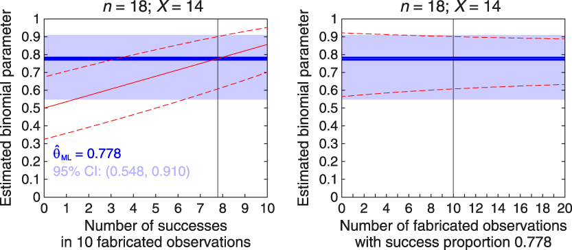
Figure 1. Effect of informative beta priors on point and interval estimates of the binomial parameter with n = 18 actual observations in which the number of successes is X = 14, so that the frequentist ML estimate is 0.778. The horizontal axis in each panel denotes prior characteristics along one of two orthogonal dimensions: The number (or proportion) of successes in a fixed number of fabricated observations (left panel) and the number of fabricated observations with a fixed proportion of successes (right panel). In the left panel, the priors are such that v + w = 12 (implying n f = 10 fabricated observations) and the abscissa represents the number v – 1 of successes in them; in the right panel, the priors are such that (v − 1)/(v + w − 2) = 0.778 (implying that the proportion of successes in fabricated data equals that in actual data) and the abscissa represents the number of fabricated observations (n f = v + w − 2). In both panels the blue horizontal line is the frequentist ML point estimate and the light blue horizontal stripe indicates the frequentist 95% score CI, neither of which varies across priors. The vertical line in each panel denotes the condition in which results in both panels meet along the two orthogonal dimensions. The continuous red line in each panel indicates the MAP Bayes estimate for each prior, and note that it sits on the blue horizontal line in the right panel; the dashed red lines in each panel indicate the lower and upper limits of the 95% HDI for each prior.
The right panel of Fig. 1 shows results as a function of the number n f of fabricated observations (ranging from 0 to 20) with prior parameters such that the proportion of successes in fabricated data always equals that in observed data. This implies a family of beta priors for which v = 1 + 0.778n f and w = n f – v + 2. By construction of the family,  ${{\rm{\hat{\theta }}}_{{\rm{MAP}}}} = {{\rm{\hat{\theta }}}_{{\rm{ML}}}}$ always and, hence, fabricated data do not alter the point estimate although the breadth of the 95% HDI decreases as the number of fabricated observations increases. Note also that n f = 0 (at the left edge of the panel) implies a uniform prior and, in these conditions, the 95% score CI and the 95% HDI still differ slightly because of the different distributions used in computations.
The families of priors used in this illustration are admittedly arbitrary but their members are realistic in the sense that the “strong prior knowledge” expected to be carried by the prior may imply a relatively large set of fabricated data with characteristics that do not match those of the actual data later collected. Discrepancies will change point estimates away from the characteristics of actual data and toward those of fabricated data, and they will also reduce the breadth of interval estimates compared to what the data alone allow. In sum, the effect of priors on point and interval estimates depends greatly on the characteristics of the implied fabricated data as a result of prior hyperparameters. This remains true even when the number n f of fabricated observations is small compared to the size n of the sample.
Bayesian estimation with uniform priors is equivalent to frequentist estimation
If the use of informative priors is equivalent to data falsification, the question arises as to whether there is any difference between frequentist estimation and Bayesian estimation with uniform priors. As shown next, the answer is that there is not any quantitative difference beyond negligible variations arising from reliance on some convenient approximations in the frequentist approach and provision of some extra flexibility in the definition of criteria for estimation in the Bayesian approach. Qualitative differences in the interpretation of frequentist and Bayesian outcomes will be discussed in the next section.
Point estimators can be arbitrarily defined according to suitable criteria and the adequacy of alternative estimators is subsequently judged on the basis of their properties (e.g., unbiasedness, consistency, efficiency, etc). Frequentists define point estimators relative to the likelihood function, which expresses the plausibility of the observed data under each of the possible values that the unknown parameter may have. Bayesians, on the other hand, define point estimators relative to a posterior distribution expressing the plausibility of each possible parameter value given the data. With uniform priors, computation of point estimators uses the exact same source and ends up with the exact same numerical result under both approaches, although the outcome may be worded differently. For instance, a frequentist will say that the ML estimate is the value of the parameter for which the observed data are most likely to have occurred; a Bayesian will say that the (identically valued) MAP estimate is the most likely value of the parameter given the observed data. The posterior distribution and the likelihood function are one and the same function when the prior is uniform (i.e., without fabricated data) and, hence, both descriptions are equally tenable whether the point estimate was computed by Bayesians or by frequentists.
As for interval estimates, frequentist CIs were defined to be dual with significance tests, in the sense that the null hypothesis that θ = θ0 is not rejected in a two-tailed size-α test only for the parameter values included in the 100(1 – α)% CI. The duality condition and the way in which two-tailed tests are conducted necessarily imply that the CI is constructed with the equal-tails criterion on the sampling distribution of the test statistic, which may on occasion be minimally different from the likelihood function of the data. However, nothing prevents frequentism from defining CIs that are not dual with significance tests or that use non-central criteria (see García-Pérez & Alcalá-Quintana, 2016). But, even without such allowance, the quantitative difference between frequentist CIs and Bayesian credible intervals is often negligible. A few examples will illustrate, all of them based on sample cases presented earlier in the context of point estimation.
Consider first interval estimation of the binomial parameter. Several significance tests exist for the binomial parameter each of which has its own dual equal-tails CI (see, e.g., García-Pérez, Reference García-Pérez2005; Newcombe, Reference Newcombe1998). Maximally accurate coverage is provided by the score CI, which comes down to the range [0.548, 0.910] when n = 18, X = 14, and α = 0.05 (i.e., the 95% CI). This CI uses the convenient normal approximation to the binomial distribution also embedded in the score test, which can be replaced without undermining the frequentist approach. One alternative is to use the skew-normal approximation instead (Chang, Lin, Pal, & Chiang, Reference Chang, Lin, Pal and Chiang2008; García-Pérez, Reference García-Pérez2009, Reference García-Pérez2010); another one is to use the CI that is dual with an exact beta test, also known as the Clopper–Pearson or exact CI. The latter 95% CI renders the interval [0.524, 0.936] for these data. As discussed above, CIs that are dual with a significance test conform to the equal-tails criterion but application of the highest-density (more precisely, highest-likelihood) principle does not oppose frequentism. This does not change the resultant score CI because it is based on a symmetric distribution, but the highest-likelihood Clopper–Pearson CI is the range [0.564, 0.922], which is the exact same range spanned by the HDI that a Bayesian would have computed using a uniform prior. On the other hand, the Bayesian equal-tailed credible interval is (0.544, 0.909), which is nearly identical to the equal-tails score CI reported earlier despite the fact that the latter uses a normal approximation to the true asymmetric distribution. Numerically, then, frequentist CIs and Bayesian credible intervals with uniform priors differ only if different criteria are used to define the intervals or if one of the computations uses exact distributions and the other uses approximations. Some of these sources of diversity may disappear in certain cases, as discussed next.
Consider now interval estimation of the mean of a normally-distributed variable. One never knows the true variance of the population and, hence, the only available option for significance testing is the one-sample t test. For the data discussed earlier (i.e., n = 30,  $\bar{X} = 43$, and $s_x^2 = 4$) the equal-tails CI spans the range [42.24, 43.76]. Identity of Bayesian equal-tailed and highest-density credible intervals holds in this case because the posterior distribution is normal (see Eq. 15). Furthermore, with a uniform prior (i.e., with n f = 0), the posterior mean is $\bar{X}$ and the posterior standard deviation is ${{\rm{\sigma }} / {\sqrt n }}$, rendering the exact same distribution that a frequentist with knowledge of σ2 would have used to compute a CI. The same knowledge of σ2 is necessary in Bayesian calculations, even with a uniform prior, but the conventional approach is to replace it with the sample variance. Then, Bayesian credible intervals are computed as CIs are by frequentists except that the referent is a normal distribution instead of a t distribution. In the preceding example, the 95% HDI spans the range (42.28, 43.72), almost identical to the 95% CI computed earlier. The minimally broader CI is easily understood because the t distribution used in its computation has heavier tails than the normal distribution with which the HDI is computed; it is not a consequence of the Bayesian approach providing more precision in any sense. Nevertheless, one could easily define frequentist CIs relative to the (scaled) likelihood function of the data which, with a uniform prior, would be identical to Bayesian credible intervals defined on the posterior.
In sum, the essence of frequentist CIs is not that they are dual with some significance test but that they are computed using only the observed data, obviously along with distributional assumptions also necessary for Bayesian computations. Then, minor quantitative differences between the limits and ranges of CIs versus credible intervals are comparable to those arising from the use of alternative criteria in either framework. Be they similar or not to CIs, it is not at all clear in what sense do Bayesian credible intervals provide better estimates. Another issue is whether both types of interval admit the same interpretation, something that is addressed in the next section.
Interpretation of frequentist and Bayesian outcomes
A bone of contention between frequentists and Bayesians is the interpretability of outcomes, particularly as regards frequentist CIs versus Bayesian HDIs. The Bayesian defense of credible intervals is that they express the probability that the parameter lies within the stated range whereas frequentist CIs are only ranges that have certain probability of containing the true parameter value. In other words, a Bayesian credible interval entails a probabilistic statement about the parameter whereas the frequentist CI entails a probabilistic statement about the interval itself. The core of the distinction lies in the Bayesian derivation of a posterior distribution for the parameter via Bayes theorem. However, as discussed earlier, the use of a uniform prior to avoid implicit data fabrication makes the posterior identical to the likelihood function, except for an inconsequential scale factor. Thus, the outcome of any frequentist computation based on the likelihood function admits the exact same interpretation as the outcome of the corresponding Bayesian computation, insofar as the former can be described as the result of Bayesian computations with a uniform prior. It is true that (dual) frequentist CIs were defined with criteria that prompt the use of sampling distributions rather than likelihood functions, but the essence of frequentism would not be undermined by defining CIs with other criteria such as, for instance, highest likelihood. For an unknown reason, frequentism is sometimes claimed to have to follow either the spirit of Fisher or that of Neymann and Pearson, on the surmise that an amalgam of both approaches is intrinsically flawed or that further development of the framework is forbidden (see, e.g., Haig, Reference Haig2017; Ivarsson, Andersen, Stenling, Johnson, & Lindwall, Reference Ivarsson, Andersen, Stenling, Johnson and Lindwall2015; Schneider, Reference Schneider2015). In contrast, and perhaps due to the posthumous publication of Bayes’ (1763) essay, the Bayesian framework had to be developed later and neglecting whether Bayes himself would have approved such developments or, at least, if he would have agreed that they bear his name (see Stigler, Reference Stigler1982). If frequentism is identically allowed development and departure from rigid adherence to its origins, there is no reason to disregard highest-likelihood CIs computed from the scaled likelihood function.
However, it is also important to unveil the underpinnings of the very notion of posterior (or prior, for that matter) distributions for the parameter of concern. It is obvious that a distributional parameter has some unknown but fixed value and, hence, that there is no such thing as a probability distribution describing the parameter in terms that are applicable only to random variables. Thus, the prior distribution only captures a researcher’s beliefs about the parameter given pre-data uncertainty about the fixed value that it may have. Naturally, the posterior is only a post-data update of such beliefs. Although this fact is not mentioned explicitly in presentations of the Bayesian approach (for an exception, see Rouder, Reference Rouder2014), it is important to realize that neither the prior nor the posterior are describing anything about the parameter of concern: They are only describing a researcher’s beliefs about plausible parameter values. Thus, a 95% HDI spanning the range, say, (0.6, 0.7) for the binomial parameter does not indicate that the parameter has probability 0.95 of being in that range (the conventional Bayesian interpretation) but, rather, that the prior and the observed data jointly prompt the researcher to believe that the parameter is in that range with probability 0.95. This is the case whether the HDI was computed with a uniform prior or with an informative prior. For a frequentist, the transgression lies in the notion that a fixed, unknown parameter value is treated as if it were a random variable with some distribution. Needless to say, everyone is free to hold beliefs and quantify them as seen fit; what is not to be expected is that researchers present beliefs and quantifications thereof as scientific evidence or results. Yet, Bayesian results that only reflect beliefs are usually presented as providing “better estimates” and “stronger inference” than would be possible under a frequentist approach. It should also be clear that the frequentist highest-likelihood CIs discussed earlier are subject to the same considerations.
Because the parameter has an unknown but fixed value, one can only aim at bracketing it within an interval computed via a procedure that can be shown to accomplish that goal with prescribed probability, and this is what frequentist CIs assure. Numerous simulation studies have shown this to hold reasonably accurately even in small-sample conditions. In contrast, aiming at statements describing the probability that the parameter lies within a certain range requires that the parameter be the random variable that it is not and, hence, such statements only represent the researcher’s beliefs about parameter values. Unsurprisingly, whether or not Bayesian HDIs accomplish their stated goal is impossible to evaluate because there is no empirical referent for “probability that the parameter is in a given range”. In these conditions, accepting a researcher’s statement that “the parameter has probability 0.95 of being in the 95% HDI” is an act of faith for everyone else.
In sum, neither frequentist nor Bayesian approaches can say anything about the probability of a parameter being within a certain range. The frequentist CI was never designed with that goal, surely due to awareness that the unknown parameter is not a random variable. The Bayesian HDI is purported to say so but the interval does not carry information on the parameter itself but on the researcher’s beliefs about it.
Discussion
The main practical difference between frequentist and Bayesian estimation is that the latter places a prior probability distribution over the parameter right before proceeding. This paper has shown that the use of informative priors in Bayesian analysis is formally equivalent to data falsification in frequentist analysis. This was shown here for conjugate priors but the same is true for non-conjugate priors although in such case the characteristics of the fabricated data cannot be directly derived. Three scenarios are thus indistinguishable: Bayesian estimation with informative priors, Bayesian estimation with uniform priors after the addition of fabricated data, and frequentist estimation after the addition of the same fabricated data. This equivalence has ramifications that should be considered both by researchers and by policy makers.
The most important implication is that the equivalence opens the door to disguising data falsification as informed Bayesian estimation. Be it deliberate, unintentional, or a byproduct of alleged Bayesian observance, data falsification is data falsification. The relevant aspect here is that the message carried by the empirical sample of observations is manipulated via addition of fake data. Strictly speaking, only the use of uniform priors can be recommended to avoid implicit data fabrication, although vague priors whose parameters make n f ridiculously small compared to n and imply fabricated data with characteristics (i.e., proportion of successes, means, etc) analogous to those of observed data are harmless in practice. Yet, a choice of such type of prior seems inconsistent with the defining goal of incorporating extant knowledge into the prior, a knowledge that may indeed be discrepant with the characteristics of data still to be collected.
This problem reaches beyond Bayesian estimation of distributional parameters and applies to all analyses in which informative priors are used (e.g., hypothesis testing, model comparisons, etc). It is worth commenting on the use of informative priors in Bayesian estimation of non-distributional parameters such as those often found in item response theory, psychophysical analysis, or structural equation modeling. In all of these cases, the parameters of concern are those describing relations among latent and observable variables and the interest lies in estimating the parameters of such relations rather than any distributional parameter of the variables themselves. The estimation problem takes a different dimension because data are only indirect indicators of the relations, which need to be inferred by fitting suitable functional models with appropriate parameters. In these conditions, data are rarely equally informative about each of the parameters in the fitted model, which hampers the estimation of some of them even when sample sizes are relatively large (for some illustrations of these problems in several areas, see García-Pérez, Reference García-Pérez2018; García-Pérez & Alcalá-Quintana, 2005, 2017; Pickles & Croudace, Reference Pickles and Croudace2010; Raykov & Marcoulides, Reference Raykov and Marcoulides2019). In the end, use of data that are uninformative about some of the parameters results in wild or boundary estimates that either look unrealistic or depart greatly from their actual values in simulation studies. There is a vast literature on this problem and one way to tackle it is to place priors on model parameters to keep the final Bayesian estimates within reasonable bounds. This strategy may or may not give acceptable results (see, e.g., Alcalá-Quintana & García-Pérez, 2004; Depaoli, Reference Depaoli2014; Finch & Miller, Reference Finch and Miller2019; Liu, Zhang, & Grimm, Reference Liu, Zhang and Grimm2016; Marcoulides, Reference Marcoulides2018; Smid, McNeish, Miočević, & van de Schoot, Reference Smid, McNeish, Miočević and van de Schoot2019) but it essentially implies injecting information through the prior to make up for the lack of it in the data. Not doing something of this sort may seem unsatisfactory in the sense that some parameter estimates will otherwise not look reasonable, but it may be more judicious to accept that the data were not informative about those parameters and to consider collecting informative data.
It should also be realized that using a prior of any type implies embracing the notion that the unknown parameter is a random variable: A probability distribution over the parameter is interpretable only in such conditions. Then, the prior (even a uniform prior) can only express a researcher’s beliefs on the plausibility of alternative values for the parameter, a subjective notion rarely mentioned in presentations of Bayesian statistics (but see Rouder, Reference Rouder2014). The immediate consequence is that Bayesian outcomes (and, particularly, Bayesian HDIs) do not indicate the range within which a parameter lies with certain probability but, rather, the range within which the researcher believes the parameter to be in under some subjective and ill-defined concept of probability. Ignoring this crucial aspect seems to justify presenting Bayesian outcomes as if they provided researchers with what they care for (namely, the probability of the parameter or hypothesis given the data) and ridded them of what the frequentist approach offers (i.e., the uninteresting probability of the data given the parameter or hypothesis). It seems perfectly acceptable for researchers to present a Bayesian quantification of their own subjective beliefs, provided that they explicitly state that this is all that they are doing; misrepresenting such quantification as if it captured some empirical reality is a breach of research integrity for which there should not be any room in the scientific literature. It is nonetheless understandable that a disdain for connections with the empirical world would reduce the perceived severity of data falsification (see Resnik, Reference Resnik2014). To avoid confusions and the misconstruction of any results that are reported with Bayesian methods, it would be desirable that such results are clearly described as portraying only the researcher’s updated beliefs given the data and the initial beliefs, which lie at an epistemological level that differs from that occupied by frequentist results that merely summarize observed data.
Criticisms of continued misinterpretation of frequentist outcomes are well-taken, particularly as regards the misconstruction of results as if they indicated the probability that a hypothesis is true or the range within which a parameter lies with some probability. Such misconstructions are often attributed to researchers’ interest in arriving at such probabilistic statements coupled with their lack of awareness that frequentism cannot provide them and with a little help from unreliable knowledge sources (see Cassidy, Dimova, Giguère, Spence, & Stanley, Reference Cassidy, Dimova, Giguère, Spence and Stanley2019). One might hope that statistical education would step in and clarify that ill-posed questions regarding the probability of hypotheses or parameter values are devoid of meaning when hypotheses and parameters are only unknowns, not random variables. Presentation of Bayesian analysis as a tool that can provide researchers with answers to such questions only contributes to statistical illiteracy.


 Open access