
Introduction
Outbreaks of insect pests such as bark beetles (Coleoptera: Curculionidae) and defoliators cause damage to Canada’s forests through growth loss and mortality (Price et al. Reference Price, Alfaro, Brown, Flannigan, Fleming and Hogg2013). The damage caused to a forest stand depends on the cumulative effect of damage to individual trees within the stand, where damage from a forest pest to a host tree is defined as any type and intensity of an effect that temporarily or permanently reduces the financial value of the tree, or impairs or removes its biological ability of growth, reproduction, and survival (Murtha Reference Murtha1972). Pest damage can therefore lead to impacts on valuable ecosystem services such as the supply of timber, and the ability of forests to sequester and store carbon, reduce flood risk, and purify water (Boyd et al. Reference Boyd, Freer-Smith, Gilligan and Godfray2013). The association of damage with impact, however, can be complicated as damage may result in a reduction in one service while increasing another. From this perspective, impact could be considered the net effect on the quantity and quality of the multiple services expected from the damaged area (adapted from Alfaro Reference Alfaro1988).
Climate change is threatening forests globally (McDowell et al. Reference McDowell, Williams, Xu, Pockman, Dickman and Sevanto2015b), and is already considered to be affecting Canada’s forests from changes to forest fire regimes, large-scale insect outbreaks, and droughts (Johnston et al. Reference Johnston, Williamson, Munson, Ogden, Moroni and Parsons2010). In particular, a changing climate is expected to amplify the impact of insect outbreaks by increasing their frequency, severity, and duration (Dale et al. Reference Dale, Joyce, McNulty, Neilson, Ayres and Flannigan2001; Volney and Fleming Reference Volney and Fleming2007; Gray Reference Gray2008; Dukes et al. Reference Dukes, Pontius, Orwig, Garnas, Rodgers and Brazee2009; Williamson et al. Reference Williamson, Colombo, Duinker, Gray, Hennessey and Houle2009; Bentz et al. Reference Bentz, Régnière, Fettig, Hansen, Hayes and Hicke2010). These potential impacts are particularly relevant for the boreal forest, where natural disturbances entailing both insects and fire largely control the interannual and interdecadal changes to its carbon balance (Bernier and Apps Reference Bernier and Apps2005). Widespread and severe damage from natural disturbances affects forest carbon dynamics of both managed and unmanaged forest areas that may reduce the ability of the forest to sequester carbon from the atmosphere (MacLean Reference MacLean1990; Alfaro Reference Alfaro1991; Bhatti et al. Reference Bhatti, van Kooten, Apps, Laird, Campbell and Campbell2003; Hicke et al. Reference Hicke, Allen, Desai, Dietze, Hall and Hogg2012; Kurz et al. Reference Kurz, Shaw, Boisvenue, Stinson, Metsaranta and Leckie2013). The combined effects of insects and fire, for example, can reportedly transform a forested region from a carbon sink to a source (Kurz et al. Reference Kurz, Dymond, Stinson, Rampley, Neilson and Carroll2008). As the climate of the planet continues to change, the direct and indirect effects of warming and natural disturbances threaten the sustainability of Canada’s forest sector (Volney and Hirsch Reference Volney and Hirsch2005). Indeed, evidence of such impacts is accumulating quickly in Canada and beyond (Gauthier et al. Reference Gauthier, Bernier, Boulanger, Guo, Guindon and Beaudoin2015; Girardin et al. Reference Girardin, Hogg, Bernier, Kurz, Guo and Cyr2015; McDowell et al. Reference McDowell, Coops, Beck, Chambers, Gangodagamage and Hicke2015a). From a global viewpoint, coping with the rising impact of forest disturbances under climate change will require the development of a modern forest health monitoring system, of which remote sensing tools will play an increasing role (McDowell et al. Reference McDowell, Coops, Beck, Chambers, Gangodagamage and Hicke2015a). A component of such a system is one focussed on mapping pest damage, which is the focus of this paper.
Information regarding the areal extent, location, and severity of insect damage is required for a range of forest pest management planning and modelling purposes (Alfaro Reference Alfaro1988; MacLean Reference MacLean1990; Wulder et al. Reference Wulder, White, Bentz and Ebata2006d; Alberta Environment and Sustainable Resource Development 2014; Westfall and Ebata Reference Westfall and Ebata2014). Across Canada, insect defoliators combined with beetles (Dendroctonus Erichson; Coleoptera: Curculionidae) and other insects, reported figures climbed from 8.8 million ha in 2012 to more than 20 million ha in 2013 (Natural Resources Canada 2015). The fact that tens of millions of hectares are being affected by major forest pests in Canada raises the need to quantify and understand their consequences on the wide range of ecosystem services that forests provide (Hicke et al. Reference Hicke, Allen, Desai, Dietze, Hall and Hogg2012; Boyd et al. Reference Boyd, Freer-Smith, Gilligan and Godfray2013). Uncertainties and knowledge gaps regarding the role of disturbances in forest ecosystem dynamics, however, create significant challenges to those charged with managing insect outbreaks (Doblas-Miranda et al. Reference Doblas-Miranda, Kneeshaw, Burton, Cooke, Fortin and MacLean2009). This problem is further complicated by how past disturbances influence future successional trajectories (Sharik et al. Reference Sharik, Adair, Baker, Battaglia, Comfort and D’Amato2010). Collecting high-quality data from long-term monitoring at different spatial and temporal scales is a prerequisite for sound pest management decisions and development of forest policies (Bechtold et al. Reference Bechtold, Tkacz and Riitters2007; Lovett et al. Reference Lovett, Burns, Driscoll, Jenkins, Mitchell and Rustad2007; Sharik et al. Reference Sharik, Adair, Baker, Battaglia, Comfort and D’Amato2010). Such information also supports analyses such as quantifying pest effects on future forest productivity (Volney and Fleming Reference Volney and Fleming2000); generating regional and national reports on the state of Canada’s forests (Natural Resources Canada 2014, 2015); quantifying natural disturbance effects on forest carbon (Kurz and Apps Reference Kurz and Apps1999); reconstructing pest outbreaks to predict future outbreaks in the context of climate change (Logan et al. Reference Logan, Régnière and Powell2003); understanding disturbance dynamics on ecosystem processes at different spatiotemporal scales (Raffa et al. Reference Raffa, Aukema, Bentz, Carroll, Hicke and Turner2008); and testing key hypotheses of forest insect population dynamics, such as the prevalence and origins of synchronised outbreak cycling behaviour (Peltonen et al. Reference Peltonen, Liebhold, Bjørnstad and Willams2002).
Pest damage information in Canada is collected using a combination of field and aerial surveys (Canadian Council of Forest Ministers 2012b). Aerial survey programmes track disturbances over space and time using maps sketched from the air by trained observers. These maps stratify the forest landscape, provide statistics regarding infested areas and trends, and identify where more precise surveys are required for pest management. The aerial maps are subjective and relatively coarse in spatial detail, however, resulting in a long-standing research interest for data from sensors mounted on aircraft or satellites (i.e., remote sensing) as a complement to aerial surveys. Remote sensing has long offered a means to quantify the frequency and extent of disturbances (McDowell et al. Reference McDowell, Coops, Beck, Chambers, Gangodagamage and Hicke2015a). While this interest has materialised in many studies, remote sensing remains a technology that is not in frequent operational use (Riley Reference Riley1989; Franklin Reference Franklin2001; Hall et al. Reference Hall, Skakun and Arsenault2007; Rullan-Silva et al. Reference Rullan-Silva, Olthoff, Delgado de la Mata and Pajares-Alonso2013). Recent reviews have attempted to identify and explain the capabilities and roles of remote sensing for forest pest damage (Wulder et al. Reference Wulder, Dymond, White, Leckie and Carroll2006a; Hall et al. Reference Hall, Skakun and Arsenault2007; Rullan-Silva et al. Reference Rullan-Silva, Olthoff, Delgado de la Mata and Pajares-Alonso2013). This paper builds from this foundation and aims at reviewing a broad range of satellite remote sensing studies encompassing both bark beetles and defoliators, examining the context of aerial surveys, discussing the problem of validating aerial surveys and remote sensing products, synthesising these studies into lessons learned, and speculating about the potential of new and upcoming remote sensing sensors and analysis approaches. More specifically, new technologies such as airborne laser scanning (ALS) and unmanned aerial vehicles (UAV) were reviewed because they offer local, above canopy perspectives of stand condition that could bridge field to satellite scales by offering data for image calibration and validation of satellite-based monitoring. Our review serves to inform how remote sensing may complement aerial and field surveys towards an integrated, multi-scale, multi-source national forest pest monitoring system.
While focussed mostly on Canada, this paper includes relevant literature from the United States of America and elsewhere for completeness. We consider nine major insect pests in Canada, including the mountain pine beetle (Dendroctonus ponderosae Hopkins (Coleoptera: Curculionidae)); spruce beetle (Dendroctonus rufipennis (Kirby)); spruce budworm (Choristoneura fumiferana (Clemens) (Lepidoptera: Tortricidae)) and western spruce budworm (Choristoneura occidentalis (Freeman)); jack pine budworm (Choristoneura pinus pinus Freeman); hemlock looper (eastern: Lambdina fiscellaria fiscellaria (Guenée) (Lepidoptera: Geometridae)) and western hemlock looper (Lambdina fiscellaria lugubrosa (Hulst)); forest tent caterpillar (Malacosoma disstria Hübner (Lepidoptera: Lasiocampidae)); large aspen tortrix (Choristoneura conflictana Walker); and gypsy moth (Lymantria dispar (Linnaeus) (Lepidoptera: Lymantriidae)). These are pests that feature most prominently in annual national and regional forest health reports over the last seven decades (Hall et al. Reference Hall, Bowers and Hirvonen1998; Simpson and Coy Reference Simpson and Coy1999; Canadian Forest Service 2013).
Major insect pests in Canada
Some knowledge of forest insect pests, and their manifestation of damage is necessary for understanding how detection and mapping by aerial survey and remote sensing is conducted. Hall et al. (Reference Hall, Skakun and Arsenault2007) suggested that a knowledge triangle comprising the insect pest, tree host, and remotely sensed image is necessary for successful use of remote sensing for detecting forest pest damage. For the purposes of detection by remote sensing, Table 1 summarises the optimal habitat, damage type, manifestation of damage, and timing for damage detection for the nine major insect pests in Canada. The timing is from the perspective of remote sensing data collection, which may be different than that required for pest management for locating insect presence on the ground.

Mountain pine beetle
The mountain pine beetle is the most damaging insect of pine (Pinus Linnaeus; Pinaceae) in western North America (Bentz et al. Reference Bentz, Régnière, Fettig, Hansen, Hayes and Hicke2010; Safranyik et al. Reference Safranyik, Carroll, Régnière, Langor, Riel and Shore2010), attacking most pine species, although it is particularly prevalent on lodgepole pine (Pinus contorta latifolia (Engelmann) Critchfield; Pinaceae). Recent outbreaks have caused widespread and severe mortality, affecting more than 18×106 ha of forest and 723×106 m3 of timber in British Columbia alone (Nealis and Cooke Reference Nealis and Cooke2014). The host range of the beetle has recently expanded from the Rocky Mountains and the southern plains regions of Saskatchewan, Canada (Cypress Hills) and North Dakota, United States of America (Black Hills) to include jack pine (Pinus banksiana Lambert) in the northern boreal plains region of Alberta (Cullingham et al. Reference Cullingham, Cooke, Dang, Davis, Cooke and Coltman2011).
Mountain pine beetles attack selected hosts en masse, overwhelming the defensive mechanisms of the tree. Directly following a successful mass attack, the foliage of the tree remains visibly unchanged. This is known as the green-attack stage, which is characterised by a decrease in sapwood moisture (Reid Reference Reid1963; Yamaoka et al. Reference Yamaoka, Swanson and Hiratsuka1990). As the tree is girdled through larval feeding on phloem, a blue-stain fungus that penetrates the xylem impedes water conductance through the outer xylem and the foliage of the crown begins to fade from green to greenish-yellow, commonly starting at the top of the tree crown (Safranyik and Carroll Reference Safranyik and Carroll2006). These trees are termed “faders”. The fading process progresses, with foliage changing from yellow to red over the subsequent spring and summer in the year following attack (Amman Reference Amman1982). Up to one year after being successfully attacked, more than 90% of killed trees will have red needles; this is known as the red-attack stage (Wulder et al. Reference Wulder, Dymond, White, Leckie and Carroll2006a). Gradually the needles will drop off the tree and typically, within three years after being attacked, most trees will have lost all their needles. This is referred to as the grey-attack stage. The rate of fade and progression through these attack stages is highly variable and depends upon a number of factors, including attack density and timing, tree moisture and condition, tree species, as well as site-specific factors (Safranyik and Carroll Reference Safranyik and Carroll2006). If peak attack occurs in July, faders may become visible in late autumn, but the bulk of the fading trees will not be detectable until the following spring (Wulder et al. Reference Wulder, Dymond, White, Leckie and Carroll2006a). If attack occurs later, then fade phenology also becomes delayed. The timing of the attack stages associated with mountain pine beetle infestation is an important operational consideration for forest health programmes, as detection from aerial survey or remote sensing data typically relies on the characteristic red-attack stage that is not reached until 6–12 months after the trees have been killed by the beetle (Table 1). Red-attack mapping will inform where trees have been attacked but it does not inform where beetles may have gone.
Detection and mitigation of beetle outbreaks typically takes advantage of the spatial correlation between red-attack and green-attack stages. Aerial survey is used to detect locations of new red-attack, with ground crews deployed to these locations to conduct ground surveys at the leading edge to detect and remove green-attack trees as a sanitation exercise to help control the outbreak (Wulder et al. Reference Wulder, Dymond, White, Leckie and Carroll2006a; Alberta Environment and Sustainable Resource Development 2014). The operational detection of green-attack with remotely sensed data is a long sought-after objective that remains elusive (Wulder et al. Reference Wulder, White, Carroll and Coops2009b). Throughout this paper and relative to mountain pine beetle, attacked trees refers to successfully mass-attacked trees for the purposes of detection, mapping, and assessment by remote sensing.
Spruce beetle
The spruce beetle is the most destructive pest of mature spruce (Picea Dietrich; Pinaceae) in western North America (Humphreys and Safranyik Reference Humphreys and Safranyik1993; Holsten et al. Reference Holsten, Their, Munson and Gibson1999). Outbreaks of this bark beetle have caused widespread mortality from Alaska, Yukon, and British Columbia, to the central Rocky Mountain states in the United States of America to Newfoundland in Canada (Holsten et al. Reference Holsten, Their, Munson and Gibson1999; Jenkins et al. Reference Jenkins, Hebertson and Munson2014). While the spruce beetle will attack all species of spruce within its range, its primary hosts include Englemann spruce (Picea engelmannii Parry ex Engelmann; Pinaceae), white spruce (Picea glauca (Moench) Voss), and Sitka spruce (Picea sitchensis (Bongard) Carrière). Spruce beetle can kill up to 90% of the trees within an infested stand during the four-year to five-year duration of a typical outbreak (Humphreys and Safranyik Reference Humphreys and Safranyik1993), which results in changes to stand structure, in particular basal area, height, and stem density (Holsten et al. Reference Holsten, Their, Munson and Gibson1999). While field information about stand characteristics such as tree canopy cover and composition has been used for rating stand susceptibility to spruce beetle infestation (Doak Reference Doak2004; Schmitt and Powell Reference Schmitt and Powell2005), there would be benefits to monitoring if similar evaluations could be done spatially using remote sensing.
Identifying spruce beetle damage and associated high-risk stands in the field is relatively straightforward compared with its detection by aerial surveys. At the beginning of an outbreak, trees remain green during the first winter, which renders early detection difficult and leads to an underestimation of mortality (Jenkins et al. Reference Jenkins, Hebertson and Munson2014). By the following July, needles will usually fade to greenish yellow and fall shortly thereafter, while the bare red twigs that remain give the crown a reddish appearance (Safranyik Reference Safranyik1995; Table 1). The four-week to six-week time window to detect the yellow-green colour of fading foliage is very narrow, and this will impact the availability of satellite images in a remote sensing application (Jenkins et al. Reference Jenkins, Hebertson and Munson2014). The optimal timing for detection is the summer following the attack (Table 1) that results in similar observations to those we made for mountain pine beetle.
Spruce budworm and western spruce budworm
The spruce budworm is considered the most destructive insect defoliator of forests in North America (Volney and Fleming Reference Volney and Fleming2007). Its primary hosts include balsam fir (Abies balsamea (Linnaeus) Miller; Pinaceae), white spruce, black spruce (Picea mariana (Miller) Britton, Sterns, and Poggenburg), and red spruce (Picea rubens Sargent) (Volney and Fleming Reference Volney and Fleming2000). The western spruce budworm is an important native defoliator of interior Douglas-fir (Pseudotsuga menziesii (Mirbel) Franco; Pinaceae) in western North America, but it can also defoliate grand fir (Abies grandis (Douglas ex Don) Lindlay), white fir (Abies concolor (Gordon and Glendinning) Lindley ex Hildebrand), subalpine fir (Abies lasiocarpa var. arizonica (Merriam) Lemmon), and many others (Fellin and Dewey Reference Fellin and Dewey1982; Volney and Fleming Reference Volney and Fleming2000). Spruce budworm outbreaks typically last 5–15 years, with several consecutive years of severe defoliation resulting in large areas of mortality and subsequent stand replacement (Fleming Reference Fleming2000). During larval feeding, residual needles become entangled with silken threads and frass, which then dry out and turn reddish-brown in colour. This colouration is used as an indicator of defoliation severity, and its occurrence governs the two to three-week period when surveys must be undertaken to assess the level of current defoliation (MacLean and MacKinnon Reference MacLean and MacKinnon1996; Table 1). However, the ability to detect spruce budworm defoliation during an aerial survey may be influenced by heavy rain washing away the discoloured dead foliage, or by the pest surveyor being unable to detect light defoliation because the proportion of discoloured foliage is very small relative to the total foliage (Fleming et al. Reference Fleming, Candau and McAlpine2002). Consecutive years of defoliation on current-year shoots result in cumulative defoliation across the younger age classes of foliage, which results in growth reduction, top-kill, and tree mortality (MacLean Reference MacLean1990; MacLean et al. Reference MacLean, Hunt, Eveleigh and Morgan1996). Cumulative defoliation in the canopy can be evaluated visually by looking up from the ground at a distance of 10–25 m against a variable sky background, which results in rough, whole-crown estimates. Other methods such as the Fettes method are used to assess cumulative defoliation at the branch level (Fettes Reference Fettes1950; MacLean and MacKinnon Reference MacLean and MacKinnon1998). The timing for mapping cumulative defoliation is towards the latter part of the summer compared to an earlier summer period used to assess current defoliation (Table 1).
Jack pine budworm
The jack pine budworm is the most damaging insect of jack pine in Canada’s boreal forest (Fleming Reference Fleming2000). Outbreaks have occurred in the forests of Ontario, Manitoba, Saskatchewan in Canada and the Great Lakes states of the United States of America (Moody Reference Moody1989). The primary host is jack pine, but red pine (Pinus resinosa Aiton), eastern white pine (Pinus strobus Linnaeus), scots pine (Pinus sylvestris Linnaeus), lodgepole pine, white spruce, black spruce, and tamarack (Larix laricina (Du Roi) Koch) have also been attacked (Ives and Wong Reference Ives and Wong1988), especially when near susceptible jack pine stands (DeBoo and Hildahl Reference DeBoo and Hildahl1968).
Jack pine budworm larvae are considered wasteful feeders, as they will feed on all but the midrib of the basal portion of the needles (McCullough Reference McCullough2000). The typical feeding pattern is from the top of the tree downwards and from the outside of the crown inwards, with wasted needles becoming entangled in a mass of silk and frass (Prebble Reference Prebble1975). As this material desiccates, it changes to a distinctive reddish-brown colour, which is a visual indicator of defoliation severity (Volney Reference Volney1988). The time period for mapping defoliation, whether by aerial survey or remote sensing, would be during this reddish-brown colour stage, which is short and ranges from late June to early July (Table 1). Several years of defoliation can result in top kill and mortality. Hall et al. (Reference Hall, Bowers and Hirvonen1998) studied the relationships between stand and site characteristics and the severity of top-kill damage, of which trees that were overmature, 15–20 m in height and growing on poor-quality sites were most likey caused by jack pine budworm defoliation. Knowledge of these associations are relevant to hazard rating and can help identify those stands where mortality from jack pine budworm defoliation could be expected to occur (McCullough et al. Reference McCullough, Marshall, Buss and Kouki1996).
Hemlock looper
The eastern and western hemlock looper are closely related allopatric subspecies that are collectively distributed across Canada from British Columbia to Newfoundland, with eastern hemlock looper extending south to Georgia in the eastern United States of America (MacLean and Ebert Reference MacLean and Ebert1999), and western hemlock looper spanning much of northwestern North America (Alfaro et al. Reference Alfaro, Taylor, Brown and Wegwitz1999). The primary hosts are balsam fir and eastern hemlock (Tsuga canadensis (Linnaeus) Carrière; Pinaceae) for eastern hemlock looper and western hemlock (Tsuga heterophylla (Rafinesque), Sargent), Engelmann spruce and white spruce for western hemlock looper, although multiple conifer and deciduous species can also be attacked during an outbreak (Alfaro et al. Reference Alfaro, Taylor, Brown and Wegwitz1999; MacLean and Ebert Reference MacLean and Ebert1999). The hemlock looper is an aggressive defoliator, with older larvae considered wasteful feeders, as they mostly feed at the base of the needle (MacLean and Ebert Reference MacLean and Ebert1999). Defoliation begins in the upper crown, with more of the tree crown being consumed at heavier population levels (Koot Reference Koot1994). As with spruce budworm and jack pine budworm, the silken threads produced by the larvae tend to catch the residual foliage, which subsequently dries and turns a dark red-brown colour (Raske et al. Reference Raske, West and Retnakaran1995) that becomes a key visual clue for aerial and remote sensing detection. Timing for detection and mapping would be at the culmination of larval feeding from mid-August to early September (Table 1). A challenge in detecting and monitoring outbreaks is that hemlock looper populations can grow rapidly, persist for one or two years, and then collapse, with host tree mortality occurring even in the first year of attack (Harris et al. Reference Harris, Dawson and Brown1982; Delisle and Hébert Reference Delisle and Hébert2012). The distribution of damage can be patchy over widespread areas, which hampers the detection of impending outbreaks (Hébert et al. Reference Hébert, Jobin, Auger and Dupont2003) from both aerial and ground surveys and remote sensing perspectives. Severe outbreaks, however, are easier to detect, as they result in high levels of mortality over limited but well-defined areas (Mills and Räther Reference Mills and Räther1990). Mature and overmature stands tend to suffer more severe damage (Delisle and Hébert Reference Delisle and Hébert2012), but there is little information about tree mortality patterns (MacLean and Ebert Reference MacLean and Ebert1999).
Forest tent caterpillar and large aspen tortrix
The forest tent caterpillar and large aspen tortrix are the most serious defoliators of trembling aspen (Populus tremuloides Michaux; Salicaceae) and balsam poplar (Populus balsamifera Linnaeus), and are a chronic pest in the prairie – boreal forest ecotone in central Canada (Peterson and Peterson Reference Peterson and Peterson1992). Both these defoliators can feed on multiple deciduous species such as white birch (Betula papyrifera Marshall; Betulaceae) and willows (Salix Linnaeus; Salicaceae), especially when populations are high (Table 1). Defoliation is best detected near the latter stages of larval feeding, approximately between mid-June to early July for the forest tent caterpillar, and early to mid-June for the large aspen tortrix (Table 1). By mid- to late July, trembling aspen with sufficient vigour will refoliate with a second flush of foliage (Ives and Wong Reference Ives and Wong1988). The severity of defoliation is therefore best observed before refoliation, which results in a very narrow time window to conduct aerial surveys or remote sensing data collection (Hall et al. Reference Hall, Skakun and Arsenault2007).
Outbreaks tend to last one to three years (rarely as long as four to six years), recur at seven-year to 13-year intervals, and are slightly less periodic and less synchronised in western Canada than in eastern Canada (Cooke et al. Reference Cooke, Lorenzetti and Roland2009). Large aspen tortrix outbreaks are short-lived, lasting two to three years, and tend to precede those of the forest tent caterpillar, with damage largely comprising reduced growth and radial increment (Cerezke and Volney Reference Cerezke and Volney1995). Populations of large aspen tortrix can rise to epidemic levels very quickly and larvae can completely strip aspen trees of foliage before the last instar, which will consequently contribute to their collapse due to starvation (Holsten et al. Reference Holsten, Hennon, Trummer, Kruse, Schultz and Lundquist2008). Drought and increasing temperatures have led to insect outbreaks resulting in defoliation, dieback, and mortality, with changes to stand dynamics throughout much of the southern boreal forest (Michaelian et al. Reference Michaelian, Hogg, Hall and Arsenault2011), including in the boreal mixedwoods (Moulinier et al. Reference Moulinier, Lorenzetti and Bergeron2013) and elsewhere (Allen et al. Reference Allen, Macalady, Chenchouni, Bachelet, McDowell and Vennetier2010).
Gypsy moth
The gypsy moth was introduced into the United States of America in the late 1860s and has since become the most destructive alien insect pest in North America, occupying most of the northeastern United States of America and eastern Canada (Liebhold et al. Reference Liebhold, Halverson and Elmes1992). While almost exclusively a deciduous defoliator, the gypsy moth has an extremely wide host base consisting of several hundred different plant species (Liebhold et al. Reference Liebhold, Elkinton and Williams2000). Its eruptive nature, wide host base, nuisance to the public, and damage to high-value urban and suburban trees explain why gypsy moth control has been a pest problem of interest.
Challenges associated with modelling gypsy moth population dynamics have led to the use of spatial defoliation data to explain and predict outbreaks (Liebhold et al. Reference Liebhold, Luzader, Reardon, Roberts, Ravlin, Sharov and Zhou1998). Aerial sketch maps have been the primary source of defoliation data, but they are limited in spatial detail, resulting in difficulties in understanding processes at a finer scale (Foster et al. Reference Foster, Townsend and Mladenoff2013). This is a particularly challenging issue, since defoliation may appear patchy within a region as a result of the mix of preferred and non-preferred host species (Nealis and Erb Reference Nealis and Erb1993). Similar to the effects of other defoliators, defoliation by gypsy moth is most obvious during the latter larval stages, when foliage consumption is maximal. Thus, the best timing for detection is during late June to early July, coincident with the culmination of larval feeding and pupation (Table 1). Light levels of defoliation may be patchy in distribution, with only moderate to severe levels considered detectable by aerial survey (Nealis and Erb Reference Nealis and Erb1993). Because this pest has such a wide host base and can feed on both deciduous and coniferous species, detection and mapping by remote sensing can be challenging, as the spectral response of the defoliated forest stands will vary by species.
Due to its eruptive potential, being aware of the location, distribution, and spread of gypsy moth in the United States of America is highly relevant to Canada. While climatic barriers and aggressive pest control have largely prevented a widespread invasion into Canada, future projections suggest a greatly increased risk to Canadian forests from this pest, particularly in western Canada (Régnière et al. Reference Régnière, Nealis and Porter2009).
Mapping damage: assessment through field and aerial surveys
Field surveys have routinely been undertaken in Canada (Hall et al. Reference Hall, Bowers and Hirvonen1998; Allen Reference Allen2001) and the United States of America (Alexander and Palmer Reference Alexander and Palmer1999) as a means to report and assess forest health. There are a multitude of methods, sampling procedures, and indicators that have been used to undertake this assessment (Ferretti Reference Ferretti1997). For example, trembling aspen defoliation has been evaluated using 10–20 randomly selected trees within sample plots, wherein trained observers inspect each tree with binoculars and assign a defoliation rating according to 10% classes (Michaelian et al. Reference Michaelian, Brandt and Hogg2001). Spruce budworm defoliation has been assessed by a trained observer dividing the living crown into thirds, and then estimating the amount of total foliage missing from the crown using binoculars (Alfaro et al. Reference Alfaro, Taylor, Brown and Clowater2001). In a study of jack pine budworm, rectangular plots were established that included ~10 sample trees from which the amount of defoliation (three classes: light, moderate, or severe) was visually assessed on current shoots (Volney Reference Volney1998). In a comparison of spruce budworm defoliation between ocular and shoot-count methods, differences were caused by observer experience, observer bias, and previous defoliation (MacLean and Lidstone Reference MacLean and Lidstone1982). MacLean and Ebert (Reference MacLean and Ebert1999) rated defoliation of hemlock looper through an ocular assessment of each tree for total defoliation and through selective branch sample assessment, from which cumulative defoliation was estimated. These examples illustrate how field procedures used to assess or rate defoliation can vary considerably. While there are some similarities between methods, they are not standardised, and their accuracy is notably affected by the observer’s experience, time available, season, weather, illumination, tree species, stand density, tree age, and the natural variation of defoliation (Heikkilä et al. Reference Heikkilä, Nevalainen and Tokola2002). To help reduce variation in observer ratings, training, calibration, and procedure documentation is essential to achieving consistent field-based health assessments.
At the landscape scale, the mapping of forest pest damage has largely been achieved by aerial overview survey (hereinafter aerial survey), which dates back at least to the 1920s, when an open-cockpit aircraft was used to map spruce budworm defoliation in portions of Québec and Ontario, Canada (Swaine Reference Swaine1921). The Forest Insect and Disease Survey was established in 1936, creating the basis for a long-term record of pest conditions (Hall et al. Reference Hall, Bowers and Hirvonen1998; Simpson and Coy Reference Simpson and Coy1999). While this long-term record allows for identifying outbreak locations and deriving trends, the individual maps are not sufficiently accurate to relate damage to impact (MacLean Reference MacLean1990). This limitation still holds even though there have been continual technical advancements that improve upon how such data are collected.
Aerial survey involves the delineation of damaged areas onto a map by a trained observer from a fixed-wing or rotary-wing aircraft, whereby the observer, using a tablet that displays a topographic map or digital imagery continually repositioned with the aid of a Global Positioning System (GPS), outlines the area of damage, rates the severity, and identifies the causal agent, which in addition to insects, may include foliar diseases and abiotic events (Brandt Reference Brandt1997; Ciesla Reference Ciesla2000). Historically, mapping was undertaken at cartographic scales ranging from 1:100 000 to 1:250 000. Finer-scale maps allow for greater accuracy and detail, with scales of 1:50 000 or finer being used for operational surveys (Resources Inventory Committee 2000). Aerial surveys are best conducted when the majority of damage is most observable. However, budget limitations, aircraft availability (especially during the fire season), or adverse weather conditions for flying may result in areas not being flown or surveyed at non-ideal times. Aerial survey is considered relatively cost effective, as information can be collected on a range of forest health concerns on an annual basis over large areas with a high likelihood of successful data acquisition (Ciesla Reference Ciesla2000; Wulder et al. Reference Wulder, White, Bentz and Ebata2006d; Hall et al. Reference Hall, Skakun and Arsenault2007).
A previous role of the Canadian Forest Service was to conduct annual insect and disease field and aerial surveys that resulted in annual regional and national reports on the state of forest pests in Canada (Brandt Reference Brandt1997; Hall et al. Reference Hall, Bowers and Hirvonen1998; Allen Reference Allen2001). This responsibility was turned over to provincial and territorial agencies in 1996 following dissolution of the Forest Insect and Disease Survey. Since then, provincial and territorial agencies conduct both field and aerial surveys over predominantly managed forests in their respective jurisdictions. The transition period for assuming this responsibility and the degree of monitoring varied by jurisdiction, resulting in data gaps for the years 1997–1999. These data gaps were particularly noteworthy in British Columbia, as it led to the absence of mountain pine beetle data in 1997 and 1998, when the outbreak was just starting. Information gaps also exist in damaged areas within and outside the managed forest (Canadian Council of Forest Ministers 2012b). Other than a composite atlas of the major forest pests in Canada from 1980 to 1996 (Simpson and Coy Reference Simpson and Coy1999), there has been no published annual report on the status of forest pests in Canada since 1995 (Hall et al. Reference Hall, Bowers and Hirvonen1998). As a result, there is a need to rely on disparate provincial survey reports, and there is no current system to compile a standardised national status report of major insect pest activity on an annual basis. A national pest strategy information system has been in development, however, which will consolidate provincial survey data into a single geospatial data model (Canadian Council of Forest Ministers 2012a).
The various methods employed in both field and aerial surveys illustrate that the approach and results depend on who is undertaking the survey and on the level of resources and training invested (note: factors governing the accuracy of an aerial survey are discussed in the Validation section). Our review of recent literature suggests that levels of survey effort vary, and that survey procedures vary by purpose (e.g., early detection versus tracking a known outbreak), resulting in challenges towards standardisation (Allen Reference Allen2001; de Beurs and Townsend Reference de Beurs and Townsend2008). Presently, 64% of the area of Canada’s managed forests, and about half of all forest lands, are monitored by aerial survey with some differences that occur from year to year as the amount of aerial coverage mapped annually may vary from province to province (Canadian Council of Forest Ministers 2012b). The occurrence of monitoring gaps results in considerable opportunities to explore the potential for complementing field and aerial surveys with remote sensing.
Mapping damage: assessment through remote sensing
There has been a limited use of remote sensing to assess insect damage, and the reported degree of success has been highly variable (Leckie and Ostaff Reference Leckie and Ostaff1988; Riley Reference Riley1989; Wulder et al. Reference Wulder, Dymond, White, Leckie and Carroll2006a; Hall et al. Reference Hall, Skakun and Arsenault2007). Reasons cited for the relatively limited use of remote sensing for forest health include perceptions of insufficient resolution of the image data (Tuominen et al. Reference Tuominen, Lipping, Kuosmanen and Haapanen2009); cost and logistics of acquiring the data; the lack of in-house expertise for processing and analysing them; and the overselling of its capabilities (Rullan-Silva et al. Reference Rullan-Silva, Olthoff, Delgado de la Mata and Pajares-Alonso2013). While there is some basis for these concerns, factors such as image resolution have become less of an issue due to the increasing availability of sensors. The incorporation of remote sensing into forest health monitoring demands an understanding of the appropriate characteristics, timing, and analysis methods of image data required for the particular forest pest problem at hand. This section answers five questions regarding these requirements, which also serve as the third component of the pest–host–image triangle:
-
1) What are the image characteristics of remote sensors?
-
2) What remote sensors are available?
-
3) What are the steps necessary to prepare remote sensing images for analysis?
-
4) What methods have been used to map pest damage?
-
5) What are some of the application examples in the literature?
What are the image characteristics of remote sensors?
Achieving a successful application of remotely sensed data requires choosing images with the appropriate image resolution characteristics from which damage can be detected. The four characteristics defining a remote sensing optical sensor include its spatial, spectral, radiometric, and temporal resolution (Lefsky and Cohen Reference Lefsky and Cohen2003).
Spatial resolution refers to the size of the ground area covered by the individual detectors of the sensor (i.e., pixel footprint), and is usually expressed as the ground spacing between the footprint centres of consecutive detectors (i.e., pixel size) (Lillesand et al. Reference Lillesand, Kiefer and Chipman2000). The pixel size of satellite remote sensing images ranges from hundreds of metres to less than a metre (Table 2). Submetric resolution sensors (i.e., pixel size <1 m) can resolve individual tree crowns and even branches, but they deliver images of reduced areal extent. For example, the 1.2-m pixel-size sensor onboard the Worldview-3 satellite has a 13.1-km swath (i.e., image width), while the 30-m OLI sensor onboard Landsat-8 has a swath of 185 km. Thus the typical trade-off is one of increased spatial resolution at the expense of decreased areal coverage. Multiple image tiles (also known as image scenes) may be required to fully capture large outbreaks. Some compromise is needed between the desired spatial resolution of the image and its extent, because multiple scenes are logistically more difficult to acquire within the narrow time frames often necessary to optimally detect the manifestation of pest damage.
Table 2 CharacteristicsFootnote * of selected current and future spaceborne optical sensors, ordered by increasing spatial resolution.Footnote ≅
Notes: * Information compiled from data on sensor specifications available from the observing systems capability analysis and review tool (http://www.wmo-sat.info/oscar) and the Earth observation (EO) portal directory (https://directory.eoportal.org).
≅ Given as ground sampling distance (i.e., pixel size). When some bands are captured at a different spatial resolution, the figure in black corresponds to the majority of bands; blue is for bands acquired at higher resolution, which also appear in blue in the “spectral region” column; red is for bands at lower resolution. Row order is based on the black figures.
⊥ Full name for sensor acronyms in the table: ASTER, advanced spaceborne thermal emission and reflection radiometer (on board NASA’s Terra); AWiFS, advanced wide field sensor (on board ResourceSat satellites); Geoeye-1 GIS, geoeye imaging system; HYPERION, hyperspectral instrument on board NASA’s EO-1; Kompsat-3 AEISS, advanced electronic image scanning system; LISS, linear imaging self-scanning sensor (on board ISRO satellites; two different sensors, LISS-3 and LISS-4); Landsat 7 ETM+, enhanced thematic mapper plus; Landsat 8 OLI, operational land imager; MODIS, moderate resolution imaging spectroradiometer (on board Terra and Aqua); Pleaides HiRi, high-resolution imager (on board Pleiades constellation); REIS, RapidEye Earth imaging system; Sentinel-2 MSI, multi-spectral imager (on board ESA’s Sentinel-2 constellation); Sentinel-3 OLCI, ocean and land colour imager (on board ESA’s Sentinel-3 constellation); SLIM6, surrey linear imager multispectral six channels (on board the Disaster Monitoring Constellation -DMC); Spot HRG, haute résolution géométrique (on board SPOT 5); Spot NAOMI, new astrosat optical modular instrument (on board SPOT 6 and 7); VÉGÉTATION-P, SPOT-VGT instrument for the PROBA-V satellite; VIIRS: visible–infrared imager radiometer suite (on board NASA and NOAA satellites; note that VIIRS has other imaging mode at 750 m with 17 bands); Worldview-3 WV110, World View 110 camera. Sensor acronyms appear in upper-case letters; for less-known sensors, the name of the carrying satellite precedes them in lowercase.
** Range (in μm) of named spectral regions: violet [0.4–0.45]; blue [0.45–0.5]; green [0.5–0.6]; red [0.6–0.7]; red edge [0.7–0.8]; pan, panchromatic [0.45–0.9] (pann: can acquire at night); VIS, visible [0.4–0.7]; NIR, near infrared [0.7–1]; SWIR, MWIR, LWIR: short-wave – mid-wave – long-wave infrared ([1–3], [3–5], [8–14]). MWIR and LWIR are TIR (thermal infrared). Unless indicated by a number (in brackets, after the region), there is one image channel per region; the spectral band covered by the channel is often narrower than the region.
≅≅ Minimum number of days between consecutive acquisitions of the same area.
⊥⊥ Availability regarding: temporal coverage (Common Era period; end of period is a rough estimate; if open, it means that sensor will continue in future satellites); spatial coverage (full: wall-to-wall, systematic; partial: scattered, on-demand); cost (free: no charge, but restrictions may apply; “$”: USD$0.01–$1/km2; “$$”: USD$1–$10/km2; “$$$”: USD$10–$50/km2. Tasked imagery usually costs twice as much as archived imagery); internet access (i.e., through a download, ordering, tasking portal: arirang: http://arirang.kari.re.kr/; dmcii: http://catalogue.dmcii.com/; eoli: http://earth.esa.int/eoli/; eotec: http://www.eotec.com/; eyefind: http://eyefind.rapideye.com/; geostore: http://www.geo-airbusds.com/geostore/; glovis: http://glovis.usgs.gov/; imagefinder: https://browse.digitalglobe.com/; laads: http://ladsweb.nascom.nasa.gov/; vito: http://www.vito-eodata.be. All websites were accessed on 6 October 2014.
*** Enabled by cross-track pointing capability; depends on latitude, maximum off-nadir angle, and number of satellites.
Optical remote sensing involves the recording and analysis of sunlight reflected by illuminated materials within the pixel footprint. The recorded response is a function of the spectral reflectance of those materials, the illumination (e.g., sun angle, viewing angle), and the atmospheric (e.g., amount of aerosols or haze/smoke) conditions at the time of image acquisition. Spectral resolution refers to the number and width of spectral bands (i.e., portions of the electromagnetic spectrum) that the sensor is able to record (Table 2). Sensors that capture a relatively large number of spectral bands of narrow width are considered to be of higher spectral resolution (Lefsky and Cohen Reference Lefsky and Cohen2003). Landsat Thematic Mapper (TM) (United States National Aeronautics and Space Institute), for example, has six bands that have an average width of over 100 nm. Thus, it is of lower spectral resolution compared with the Hyperion (United States National Aeronautics and Space Institute) sensor, which has 220 bands that are 10 nm wide (Pearlman et al. Reference Pearlman, Barry, Segal, Shepaanski, Beiso and Carman2003) and can detect subtle differences between similar surface materials that are not detectable using the broad Landsat TM bands. Satellite sensors such as the Hyperion are known as hyperspectral and up to now were largely experimental, although there are new missions planned (e.g., HyspIRI – Hyperspectral Infrared Imager) (Bioucas-Dias et al. Reference Bioucas-Dias, Plaza, Camps-Valls, Scheunders, Nasrabadi and Chanussot2013). The suitability of a given sensor for mapping insect damage is a function of the interrelationship between spectral and spatial resolution. For a given pixel, its spectral response is a function of the spectral reflectance of the illuminated surfaces of the objects within the pixel footprint. The larger the pixel, the greater the number of distinct surface materials that contribute to the overall pixel response. In order for a sensor to be able to detect insect damage, its effect on the spectral response of the pixel must be larger or more dominant than that of those materials within the pixel unaffected by the damage.
Radiometric resolution is the number of intensity levels in which the radiance received by the sensor in a given spectral band is quantised. These “grey levels” are stored pixel by pixel as digital numbers that represent the ability of the sensor to discriminate small differences in incoming radiance from adjacent pixels (Lillesand et al. Reference Lillesand, Kiefer and Chipman2000). For example, Landsat 5 and 7 are quantised to a bit depth of eight bits, or 256 grey levels (Lefsky and Cohen Reference Lefsky and Cohen2003). While eight-bit radiometric resolution was common for earlier sensors, current and upcoming sensors have higher bit depths, ranging from 10 to 12 bits, that is, 1024 and 4056 grey levels, respectively (Table 2). These higher radiometric resolution sensors potentially translate to higher sensitivity to differences in reflectance between healthy and damaged vegetation. While radiometric resolution was not an issue of concern in past studies of forest disturbance (Coops et al. Reference Coops, Wulder and White2007), future remote sensing of pest damage will be based on the 12-bit generation of sensors such as Landsat 8’s Operational Line Imager (OLI) and Sentinel-2 Multi-Spectral Imager (MSI).
Temporal resolution, or revisit time, is the number of days for which a particular sensor will be able to obtain new imagery (cloud-free or not) over a particular area of interest (Lefsky and Cohen Reference Lefsky and Cohen2003). Higher temporal resolution usually comes at the expense of coarser spatial resolution, although many of the newer satellites with metric (pixel size 1–9 m) or submetric (<1 m) resolution sensors can have higher revisit times because they have pointable sensor heads and (or) are concurrently carried by a constellation of satellites. A trade-off of this acquisition mode, is however, that the area of interest could be imaged at an oblique angle of view, which can lead to radiometric and geometric distortions (Wulder et al. Reference Wulder, White, Coops and Butson2008c). In order to monitor disturbances such as bark beetle outbreaks, images acquired in different years corresponding to before and after the outbreak are often employed (Coops et al. Reference Coops, Wulder and White2007). These “anniversary date” images need to be acquired at approximately the same time of year to minimise differences in solar illumination and vegetative phenology. The opportunity to acquire image data timed to when pest damage is visible is increasing with new satellites such as with Landsat 8 and Sentinel 2 (Table 2).
What sensors are available?
There is a plethora of sensors that can be applied to forest pest damage. Here we will focus on spaceborne sensors, because they produce images that have consistent spatial resolution and several are cost-free (for information on digital aerial cameras, see Jacobsen Reference Jacobsen2010). There are dozens of civilian satellites acquiring images around the Earth every day, or hundreds if past missions are considered (Kramer Reference Kramer2002). The number of operational Earth observation (EO) satellites has increased substantially in recent years thanks to new technological developments that enabled the deployment of affordable small satellite missions (Sandau Reference Sandau2010; Argoun Reference Argoun2012). A sample of 21 spaceborne optical sensors, current and future, appears in Table 2, along with information on different types of resolution and availability. Spectral resolution varies from the three bands of LISS-4 to the 220 bands of Hyperion (Table 2). Radiometric resolution goes from 256 grey levels (8-bit) in Landsat TM imagery to 65 536 (16-bit) in RapidEye. Spatial resolution ranges from two-thirds of a kilometre in Vegetation-P to one-third of a metre in Worldview-3 pan. Image width (i.e., swath) can go from as little as 13 km (Worldview-3) to as much as 3000 km (VIIRS). Images of a given location can be acquired as frequently as daily (many sensors) to only every 24 days (LISS-3). Archived imagery from most sensors can be searched and ordered online from dedicated web map interfaces. New imagery can be downloaded just a few days after it was acquired. When the sensor works only on demand, tasking orders for a particular project may be placed online or through toll-free order desks, and the images delivered just a few days after successful acquisition. Imagery of 30-m spatial resolution and coarser is now free of charge, especially since the opening of the Landsat archive in 2008 (Wulder et al. Reference Wulder, Masek, Cohen, Loveland and Woodcock2012a).
Sensors that have been most frequently used in studies of remote sensing change detection are those operating on a systematic, full coverage basis such as Landsat (TM, ETM+, and their successor, OLI; Roy et al. Reference Roy, Wulder, Loveland, Woodcock, Allen and Anderson2014) and MODIS (to be replaced by VIIRS; Justice et al. Reference Justice, Vermote, Privette and Sei2011). Hectometric imagery like MODIS (i.e., with spatial resolution on the order of hectometres; i.e., 100 m) can be used to precisely locate in time changes in vegetation that occur concurrently over very large areas, such as autumn’s leaf abscission, since the larger number of revisits increases the likelihood of securing relatively cloud-free image data over the area of interest (Reed et al. Reference Reed, Schwartz and Xiao2009). However, there are limitations to using such imagery for detecting pest damage. In the early stages of an outbreak, individual coarse pixels are likely to contain relatively large amounts of unaffected vegetation or unsusceptible cover that will hamper detection. In general, imagery from sensors such as MODIS has been found useful for detecting insect damage over large spatial scales, but not for estimating its severity (e.g., van der Sanden et al. Reference van der Sanden, Deschamps, Thomas, Landry and Hall2006; Eklundh et al. Reference Eklundh, Johansson and Solberg2009).
Of all sensors, the ones that have been most frequently employed for pest damage assessment are those onboard the Landsat series (Wulder et al. Reference Wulder, White, Bentz, Alvarez and Coops2006c; Hall et al. Reference Hall, Skakun and Arsenault2007; Rullan-Silva et al. Reference Rullan-Silva, Olthoff, Delgado de la Mata and Pajares-Alonso2013), which have a spatial resolution (30 m) and swath (185 km) suitable for damage mapping at the stand level, although their 16-day revisit time can limit detection opportunities for tree species that re-flush after defoliation. For example, the late June to early July peak defoliation period for forest tent caterpillar throughout much of the Canadian boreal forest is followed by refoliation by aspen in late July, meaning that there are only two or three chances to obtain clear-sky Landsat observations before defoliation is no longer visible (Hall et al. Reference Hall, Skakun and Arsenault2007). Other decametric sensors (i.e., with spatial resolution on the order of decametres), such as those in SPOT satellites, can provide shorter revisit times by “pointing” the sensor cross-track to collect off-nadir imagery (Moran et al. Reference Moran, Jackson, Clarke, Qi, Cabot and Thome1995). Off-nadir viewing can, however, introduce radiometric distortion to the imagery, such as increased effects of bidirectional reflectance, that would create difficulties when implementing change detection techniques, particularly if the off-nadir look-angle was not consistent between pre-damage and post-damage images (Asner and Warner Reference Asner and Warner2003; Davi et al. Reference Davi, Soudani, Deckx, Dufrene, Le Dantec and Francois2006).
Despite data gaps due to the failure, since May 2003, of the scan-line corrector of the Landsat 7 ETM+ sensor, the launch of OLI on board Landsat-8 in February 2013 has guaranteed the continuity of an over 40-year Landsat record that has greatly advanced science and monitoring applications, and that is available to the public free of charge since 2008 (Wulder et al. Reference Wulder, Masek, Cohen, Loveland and Woodcock2012a; Roy et al. Reference Roy, Wulder, Loveland, Woodcock, Allen and Anderson2014). To further extend the value of the Landsat 7 ETM+ sensor for forest change applications, various gap-filling algorithms have been developed and evaluated (Wulder et al. Reference Wulder, Ortlepp, White and Maxwell2008b; Chen et al. Reference Chen, Zhu, Vogelmann, Gao and Jin2011; Zeng et al. Reference Zeng, Shen and Zhang2013). Monitoring capabilities from Landsat sensors will be improved by the Sentinel-2 constellation, which will offer a similar multispectral sensor (MSI, Table 2) but with a 290 km swath and a higher revisit rate of five days under the same viewing conditions (Drusch et al. Reference Drusch, Del Bello, Carlier, Colin, Fernandez and Gascon2012). Sentinel-2A was successfully launched 23 June 2015, marking the beginning of a new era of increased EO capabilities with the combination of Landsat 8 and Sentinel-2.
In addition to better spatial and temporal resolution, the Sentinel-2 Multi-Spectral Imager has three bands covering the red-edge region (0.7–0.8 μm) as opposed to no coverage in OLI. This will enable the detection of stress-induced shifts in the spectral signature of vegetation in the red edge that are suitable for early forest damage detection (Rullan-Silva et al. Reference Rullan-Silva, Olthoff, Delgado de la Mata and Pajares-Alonso2013). Other future missions (e.g., HyspIRI; not shown in Table 2) include hyperspectral sensors that would allow computing narrow-band indices such as the structure-insensitive pigment index (SIPI; Peñuelas et al. Reference Peñuelas, Baret and Filella1995), which has the potential to detect early decline symptoms in vegetation (Pontius Reference Pontius2014).
Metric (1–9 m) and submetric (<1 m) resolution sensors enable the assessment of damage at the plot (or even individual tree) level by acquiring image data on-demand, and even if they have a narrow swath (typically <20 km for submetric imagery), they can repeatedly acquire new images every few days thanks to their cross-track pointing capabilities. The availability of archived imagery, however, is typically inconsistent and incomplete, except perhaps in urban and other high-demand areas. Operational mapping of large regions would be cost prohibitive, since large numbers of images would be required, and logistically more difficult to acquire because of the need to “task” (i.e., preorder) image acquisition (White et al. Reference White, Wulder, Brooks, Reich and Wheate2005). Off-nadir view angles, which result in geometric distortion of trees and high contrast between sunlit and shadow portions of tree crowns, also complicate the use of change detection methods when applied to such data (Peddle et al. Reference Peddle, Franklin, Johnson, Lavigne and Wulder2003; Im and Jensen Reference Im and Jensen2005). Notwithstanding these issues, the use of submetric imagery may be warranted for calibration and validation of damage models derived from coarser imagery, when the finer spatial resolution imagery is only available for a portion of the area of interest (e.g., Meddens et al. Reference Meddens, Hicke, Vierling and Hudak2013).
What are the steps necessary to prepare remote sensing images for analysis?
While forest pest damage may be detected in a single remote sensing image, tracking damage requires images from two or more dates. Ensuring good alignment and radiometric consistency between the images is a prerequisite to successful change detection. Typical preprocessing steps include geometric correction and image-to-image registration, topographic correction, and radiometric and atmospheric corrections (Lu et al. Reference Lu, Mausel, Brondizio and Moran2004). Such procedures are relevant for consistently detecting both gradual and abrupt changes caused by insect pests, especially since bark beetles and defoliators exhibit a wide range of damage patterns (Ives and Wong Reference Ives and Wong1988; Armstrong and Ives Reference Armstrong and Ives1995). There are a number of geometric correction methods for digital images whose selection depend somewhat on the intended use of the image (Toutin Reference Toutin2004). There is consensus that subpixel registration accuracies are preferred for change detection, that is, the distance between the actual footprint centres of collocated pixels should be on average less than the pixel size (Coppin et al. Reference Coppin, Jonckheere, Nackaerts and Muys2004).
Slope and topography will influence the amount of reflected radiation received by the sensor, which can complicate the detection of forest damage (Ekstrand Reference Ekstrand1996). For example, different methods for topographic correction of Landsat TM imagery were evaluated and shown to influence the mapping of vegetation types (Riaño et al. Reference Riaño, Chuvieco, Salas and Aguado2003). Healthy to slightly defoliated forest was successfully separated from moderately defoliated forest when a model accounting for topographic effects was employed (Ekstrand Reference Ekstrand1996). In a bitemporal study that compared combinations of atmospheric and topographic corrections with no corrections, corrected images resulted in higher land cover classification accuracies (Vanonckelen et al. Reference Vanonckelen, Lhermitte and Van Rompaey2013). These studies support the rationale that accounting for topography would improve consistency for mapping forest damage.
Satellite images are subject to atmospheric effects and variations in sensor response that require corrections before analysis (Peddle et al. Reference Peddle, Franklin, Johnson, Lavigne and Wulder2003). Spectral bands in the visible portion of the spectrum are more sensitive to atmospheric effects than those in the near and shortwave infrared, which may cause spurious variations in vegetation indices that combine both types of bands (Liang et al. Reference Liang, Fang, Morisette, Chen, Shuey and Walthall2002). Seasonal phenology and variability in ground conditions could also create differences in the spectral responses (Song and Woodcock Reference Song and Woodcock2003) that may have little to do with change associated with the disturbance. When analysing a multitemporal data set, some level of radiometric correction is considered necessary to differentiate real change from noise (Schroeder et al. Reference Schroeder, Cohen, Song, Canty and Yang2006). Employing change detection methods generally requires either an absolute correction for atmospheric effects or a relative correction (i.e., normalisation through pseudo-invariant features such as barren lands) between the two or more images that represent pre- and post-disturbance stages (Song et al. Reference Song, Woodcock, Seto, Lenney and Macomber2001; Coppin et al. Reference Coppin, Jonckheere, Nackaerts and Muys2004; Lu et al. Reference Lu, Mausel, Brondizio and Moran2004). Ensuring the comparability of multitemporal data sets requires some level of radiometric correction procedures (Vicente-Serrano et al. Reference Vicente-Serrano, Pérez-Cabello and Lasanta2008), which would be particularly relevant when analysing gradual changes in vegetation cover such as defoliation. For example, a simple relative normalisation between two images was successfully applied to forest mortality mapping by only applying histogram matching between pseudo-invariant targets (e.g., deep water, healthy vegetation) (Collins and Woodcock Reference Collins and Woodcock1996).
Methods and/or correction coefficients have been published for many radiometric correction techniques, including conversion to top-of-atmosphere reflectance (Chander and Markham Reference Chander and Markham2003; Chander et al. Reference Chander, Markham and Barsi2007), dark-object subtraction (Chavez Reference Chavez1988; Teillet and Fedosejevs Reference Teillet and Fedosejevs1995), measuring or estimating atmospheric aerosols to derive surface reflectance (Liang et al. Reference Liang, Fang and Chen2001; Thome Reference Thome2001), applying radiative transfer functions (Moran et al. Reference Moran, Jackson, Slater and Teillet1992), empirical line calibration (Moran et al. Reference Moran, Bryant, Thome, Ni, Nouvellon and Gonzalez-Dugo2001), and haze removal (Richter Reference Richter1996). More detailed reviews and summaries of radiometric image processing entailing terminology, sensor radiometric calibration, surface reflectance retrieval, image normalisation, and topographic corrections are available from Richards and Jia (Reference Richards and Jia1999), Liang et al. (Reference Liang, Fang and Chen2001, Reference Liang, Fang, Morisette, Chen, Shuey and Walthall2002), Peddle et al. (Reference Peddle, Franklin, Johnson, Lavigne and Wulder2003), Schaepman-Strub et al. (Reference Schaepman-Strub, Schaepman, Painter, Dangel and Martonchik2006), and Vanonckelen et al. (Reference Vanonckelen, Lhermitte and Van Rompaey2013). Atmospheric correction is considered essential if multiband ratioing such as vegetation indices will be used in the detection of change (Gong and Xu Reference Gong and Xu2003). Thus, while the selection of the appropriate level of atmospheric processing does depend on the intended application and the nature of the disturbance being detected, the general consensus is that radiometric and atmospheric corrections should be considered when analysing multitemporal images (Lunetta and Elvidge Reference Lunetta and Elvidge1999; Schroeder et al. Reference Schroeder, Cohen, Song, Canty and Yang2006; Coops et al. Reference Coops, Wulder and White2007).
What methods have been used or are relevant to forest pest damage?
While some forest pest damage patterns may be detected using a single date image, employing two or more image dates is in general more reliable. There is a plethora of change detection methods in the remote sensing literature (see reviews by Singh Reference Singh1989; Coppin et al. Reference Coppin, Jonckheere, Nackaerts and Muys2004; Lu et al. Reference Lu, Mausel, Brondizio and Moran2004; Hussain et al. Reference Hussain, Chen, Cheng, Wei and Stanley2013). Unfortunately, there is no universal change detection method (Tewkesbury et al. Reference Tewkesbury, Comber, Tate, Lamb and Fisher2015), and no single approach is optimal and applicable to all cases (Lu et al. Reference Lu, Mausel, Brondizio and Moran2004). As a result, selecting a suitable change detection approach for a particular area and problem can be challenging (Lu et al. Reference Lu, Li and Moran2014). A general procedure for conducting a change detection analysis was presented by Lu et al. (Reference Lu, Li and Moran2014), whose major steps include: (1) describing the change detection problem; (2) selecting suitable remotely sensed data; (3) conducting image preprocessing; (4) selecting suitable variables; (5) selecting a suitable change algorithm; and (6) evaluating change detection results. It is important to stress that the last step calls for linking the change detected on the image to observations on the ground, which in turn requires field data collection and characterisation of forest condition. An approach for selecting a change detection method for forest pest damage assessment is to review past experiences from which to summarise methods used and results attained. From this perspective, what are the change detection methods that have been applied to studies of pest damage?
We compiled a list of remote sensing studies from Canada and the United States of America dealing with change detection and created a table that describes the different methods, including their advantages and disadvantages (Table 3). The methods were stratified into five groups that we labeled as visual analysis, image algebra, classification, spectral mixture analysis, and time series analysis. Together, they exemplify the change detection methods that have been applied to studies of pest damage. Consistent with previous observations (Hall et al. Reference Hall, Skakun and Arsenault2007), image differencing of vegetation indices based on spectral band ratios have been most frequently employed. This approach, also called layer arithmetic, is among the simplest and most frequently used method of bitemporal change detection (Lu et al. Reference Lu, Mausel, Brondizio and Moran2004; Tewkesbury et al. Reference Tewkesbury, Comber, Tate, Lamb and Fisher2015). The challenge with this approach is in defining the threshold value to the magnitude of change (Hussain et al. Reference Hussain, Chen, Cheng, Wei and Stanley2013) that represents a meaningful change in terms of for example, insect defoliation, which calls for associating field-measured estimates of percent defoliation to changes in the image.
Table 3 Some change detection techniques that have been applied to the mapping of forest pest damage.Footnote *
* Sources: Coppin et al. (Reference Coppin, Jonckheere, Nackaerts and Muys2004), Lu et al. (Reference Lu, Mausel, Brondizio and Moran2004), Hussain et al. (Reference Hussain, Chen, Cheng, Wei and Stanley2013).
A review of Table 3 suggests change detection methods are evolving. Change detection was based on the detection of change between image dates timed to observe spectral response differences in variables of interest such as insect damage. More recent studies are investigating the use of multiple image dates to track a more continuous time series of pixel spectral response as a function of ecosystem dynamics. By integrating multiple image dates, factors such as growth trajectories, phenology, climate effects, and natural and anthropogenic disturbances can also be considered as these will influence changes in the forest landscape in addition to those caused by insect damage (Table 3). This trend is consistent with directions toward annual land cover classification maps that incorporate change information by tracking disturbance and recovery derived from long time series of satellite imagery (Franklin et al. Reference Franklin, Amed, Wulder, White, Hermosilla and Coops2015).
What are some of the application examples in the literature?
We reviewed a number of studies dealing with the application of remote sensing to forest pest damage, which include those cited in previous pest-related remote sensing reviews (Wulder et al. Reference Wulder, Dymond, White, Leckie and Carroll2006a; Hall et al. Reference Hall, Skakun and Arsenault2007; Rullan-Silva et al. Reference Rullan-Silva, Olthoff, Delgado de la Mata and Pajares-Alonso2013). In the following subsections, we briefly review the historical evolution of this field, summarise remote sensing studies for both bark beetles (Table 4) and defoliators (Table 5), and offer an overview of emerging remote sensing technologies.
Table 4 Remote sensing studies applied to two bark beetles.
Notes: * “AC” indicates that atmospheric correction procedures were employed.
DI, disturbance index; EWDI, enhanced wetness difference index; NDMI, normalised difference moisture index; RGI, red–green index; USA, United States of America.
Table 5 Remote sensing studies applied to seven insect defoliators (updated from Hall et al. Reference Hall, Skakun and Arsenault2007).
Notes: * AC, atmospheric correction procedures were employed.
DI, disturbance index; LAI, leaf area index; SWIR/NIR, shortwave infrared – near infrared; VI, vegetation index; USA, United States of America.
Brief historical review
Before the availability of satellite data, early studies on forest pest damage were undertaken with aerial photographs taken mostly from fixed-wing and rotary-wing aircraft. Among the first studies in both Canada and the United States of America were the following: damaged and defoliated trees were reported to be darker than healthy trees on black and white infrared photographs (Spurr Reference Spurr1946); a comparison of panchromatic, infrared, colour, and colour infrared aerial films at three scales was undertaken for assessing damage from western pine beetle (Dendroctonus brevicomis LeConte (Coleoptera: Curculionidae)) (Wear and Bongberg Reference Wear and Bongberg1951); an evaluation of camera systems was completed for low-altitude sampling of forest insect damage (Heller et. al. Reference Heller, Aldrich and Bailey1959a); and the interpretation of aerial photography for detecting southern pine beetle (Dendroctonus frontalis Zimmermann) damage (Heller et al. Reference Heller, Aldrich and Bailey1959b). Subsequent work included using colour and panchromatic aerial photographs to survey mortality caused by Douglas-fir beetle (Dendroctonus pseudotsugae Hopkins) (Wear et al. Reference Wear, Pope and Lauterback1964); surveying the amount of Douglas-fir beetle mortality from 1:8000 large-scale aerial photographs (Wert and Roettgering Reference Wert and Roettgering1968); detecting conifer damage using near-infrared film (Murtha and Hamilton Reference Murtha and Hamilton1969); assessing insect damage from high-altitude colour infrared photographs (Ciesla Reference Ciesla1974); evaluate small-scale (1:137 000) colour aerial photos for forest pest surveys (Harris Reference Harris1974); and quantifying gypsy moth defoliation from colour and colour infrared photography (Talerico et al. Reference Talerico, Walker and Skratt1978), to list but a few. Along with these early studies, Murtha (Reference Murtha1969) began developing the conceptual foundation for aerial photograph interpretation of forest damage. This work led to a key publication that served as the fundamental guide for air photograph interpretation of forest damage (Murtha Reference Murtha1972). These reports contributed to the fundamental theory for remote sensing damage assessment based on aerial photographs, and the need to understand how physiological and morphological damage to trees from forest pests are manifested in terms of changes to the spectral reflectance patterns of forest vegetation (Murtha Reference Murtha1976, Reference Murtha1978; Puritch Reference Puritch1981).
The launch of the Earth Resources Technology Satellite (ERTS-1, later renamed Landsat 1) in 1972 marked the beginning of the Landsat satellite collection of EO data, which has been of primary interest in studies of forest insect damage. Early studies include: the mapping of hemlock looper damage from ERTS-1 imagery (Beaubien and Jobin Reference Beaubien and Jobin1974); an evaluation of Landsat data for forest pest detection (Harris et al. Reference Harris, Dawson and Goodenough1978); and use of pre-outbreak and post-outbreak Landsat imagery to detect gypsy moth defoliation (Dottavio and Williams Reference Dottavio and Williams1983). A compilation of papers describing the early use of EO data for monitoring forest insect damage was presented in a landmark symposium on remote sensing for vegetation damage assessment organised by the American Society of Photogrammetry held in Seattle, Washington, United States of America, in 1978 (Heller Reference Heller1978; Murtha Reference Murtha1978; Williams and Stauffer Reference Williams and Stauffer1978). Over the years since, remote sensing of insect damage has demonstrated considerable potential but with variable reported success (Leckie and Ostaff Reference Leckie and Ostaff1988; Riley Reference Riley1989; Franklin Reference Franklin2001; Hall et al. Reference Hall, Skakun and Arsenault2007; Rullan-Silva et al. Reference Rullan-Silva, Olthoff, Delgado de la Mata and Pajares-Alonso2013), which can be attributed to several factors. First, there is no single, most suitable way to inventory and monitor pest damage using remote sensing, as the manifestation of damage is host and pest specific (Murtha Reference Murtha1976). Second, the optimal timing of when damage is most visible is often narrow, which can challenge the acquisition of cloud-free satellite data. Third, forest damage is typically mapped into a few discrete, subjectively derived damage classes specifying light, moderate, and severe damage, which oversimplifies the reality that damage occurs as a continuum. All these factors complicate the association of remote sensing observations to field and aerial assessments of forest condition. As a result, despite the apparent high potential for use of remote sensing to map insect damage, it remains a technology that has seen relatively little operational use (Peterson et al. Reference Peterson, Resetar, Brower and Diver1999; Franklin Reference Franklin2001; Hall et al. Reference Hall, Skakun and Arsenault2007; Hicke et al. Reference Hicke, Allen, Desai, Dietze, Hall and Hogg2012).
Our review of the literature on the use of remote sensing for bark beetle damage and insect defoliation suggests that for a specific pest damage problem (e.g., spruce budworm defoliation), no consistent approach has been employed (Tables 4 and 5). The mountain pine beetle has received more attention than defoliators, and methods employed depend highly on the objective of the analysis and data sources available. To summarise insights into research findings and advances, a review of papers, mostly satellite-based plus a few airborne, were selected to illustrate applications of remote sensing to this subject (Tables 4 and 5).
Bark beetles
There are many studies that have employed a range of remotely sensed data sources to detect and monitor damage caused by the mountain pine beetle, particularly in Canada, and less so for spruce beetle (Table 4). Research into methods for large-area mapping of mountain pine beetle red-attack damage historically focussed on the use of aerial photography (see Wulder et al. Reference Wulder, Dymond, White, Leckie and Carroll2006a for a detailed review). However, the recent extensive outbreak of mountain pine beetle in western North America, which started in the late 1990s, prompted considerable Canadian research into the use of satellite remote sensing to map epidemic levels of red-attack damage over large areas (Franklin et al. Reference Franklin, Wulder, Skakun and Carroll2003; Skakun et al. Reference Skakun, Wulder and Franklin2003; White et al. Reference White, Wulder and Grills2006; Wulder et al. Reference Wulder, White, Bentz, Alvarez and Coops2006c; Coops et al. Reference Coops, Waring, Wulder and White2009b). Franklin et al. (Reference Franklin, Wulder, Skakun and Carroll2003) used a single date of Landsat TM imagery to map areas of red-attack with an overall accuracy of 72%. Skakun et al. (Reference Skakun, Wulder and Franklin2003) used multiple dates of Landsat TM and ETM+ imagery and the enhanced wetness difference index (EWDI) to map red-attack damage severity. The EWDI is calculated by subtracting the tasseled cap wetness index (Crist and Cicone Reference Crist and Cicone1984) from two images, which are preferably acquired two years apart. With this approach, it was found that areas with severe damage (represented in the GIS reference data as scattered points, each with 30–50 red-attack trees in their surroundings) were mapped with greater accuracy (producer’s accuracy=78%; user’s accuracy=81%) than areas with moderate damage (10–29 red-attack trees per GIS point; producer’s accuracy=68%; user’s accuracy=76%). Producer’s accuracy represents a measure of omission error that describes the probability of a reference pixel being correctly classified whereas user’s accuracy indicates commission error that describes the probability a pixel classified on the image actually represents that category on the ground (Congalton and Green Reference Congalton and Green2009). Wulder et al. (Reference Wulder, White, Bentz, Alvarez and Coops2006c) used the EWDI in a logistic regression approach to map red-attack damage in a mixed forest environment with variable terrain. Slope and solar radiation were also incorporated into the logistic model and resulted in a producer’s accuracy of 83% (user’s accuracy=88%) for detection of red attack. While operational objectives would govern which level of accuracy is required for pest management decisions, these studies do illustrate the degree to which red-attack damage can be mapped using various methods with single or multiple date Landsat TM/ETM+ images.
With free and open access to the Landsat archive since 2008, research has increasingly explored the use of a time series of Landsat data to detect and map damage caused by mountain pine beetle (Goodwin et al. Reference Goodwin, Coops, Wulder, Gillanders, Schroeder and Nelson2008, Reference Goodwin, Magnussen, Coops and Wulder2010; Meigs et al. Reference Meigs, Kennedy and Cohen2011; Meddens et al. Reference Meddens, Hicke, Vierling and Hudak2013). Time series analysis allows identification of the year in which mortality occurred, a critical piece of information for salvage harvesting and fire risk modelling, among others. Using eight Landsat images acquired between 1992 and 2006, Goodwin et al. (Reference Goodwin, Coops, Wulder, Gillanders, Schroeder and Nelson2008) used the normalised difference moisture index (NDMI; Wilson and Sader Reference Wilson and Sader2002) to identify red-attack damage over a 1.5 million ha area in north-central British Columbia. Detailed helicopter survey data from 1996, 2003, and 2004 were used for validation, and red-attack detection accuracies were 49% in 1996, 79% in 2003, and 78% in 2004. Meigs et al. (Reference Meigs, Kennedy and Cohen2011) used the LandTrendr algorithm (Kennedy et al. Reference Kennedy, Yang and Cohen2010) over the Cascade Range in Oregon, United States of America to characterise mortality induced by bark beetle, finding a statistically significant relationship between field-based measures of severity (total basal area killed) and Landsat spectral change (accuracy of red-attack detection not reported). Meddens et al. (Reference Meddens, Hicke, Vierling and Hudak2013) explicitly compared the performance of single-date and multitemporal approaches over a study area in northcentral Colorado and southern Wyoming, United States of America, and found that both had comparable accuracies, but concluded that trajectory-based methods were more effective for mapping intermediate levels of mortality, whereas single-date methods were more effective at mapping high levels of mortality. Producer’s accuracies for red attack ranged from 83% to 88% for single-date methods and 85–87% for multidate methods. Therefore, single date methods can be combined with multitemporal methods to enhance accuracy of both high and low levels of damage.
While large area maps of mountain pine beetle red-attack damage derived from Landsat imagery provide essential strategic-level information (Wulder et al. Reference Wulder, White, Bentz and Ebata2006d), higher spatial resolution satellite imagery provides detailed information over specific areas that are of value to direct mitigation efforts. White et al. (Reference White, Wulder, Brooks, Reich and Wheate2005) used IKONOS 4-m multispectral data to map low (between 1% and 5% of the stand is infested) and medium (between 5% and 20% of the stand is infested) levels of red-attack damage in central interior British Columbia forest stands with producer’s accuracies for red attack of 71% and 92%, respectively. Coops et al. (Reference Coops, Johnson, Wulder and White2006a) used 2.5-m QuickBird imagery and the red–green index (RGI) in northeastern British Columbia to map red-attack damage and found a significant relationship between the number of red-attack pixels and number of field-surveyed red-attack tree crowns (R 2=0.48, P<0.001, standard error=2.8 crowns) (accuracy of red-attack detection not reported). Also in British Columbia, Wulder et al. (Reference Wulder, White, Coops and Butson2008c) used multitemporal QuickBird imagery to retrospectively reconstruct the gradual increase in mortality from 2003 to 2006 with producer’s accuracies for red-attack detection ranging from 89% to 93%. Hicke and Logan (Reference Hicke and Logan2009) used QuickBird imagery and the RGI to map red-attack damage in stands dominated by whitebark pine with a producer’s accuracy for red-attack detection of 84%. Dennison et al. (Reference Dennison, Brunelle and Carter2010) used GeoEye-1 data, which has a 0.5-m spatial resolution, to map both red-attack and grey-attack damage and reported a strong relationship between field-measured tree-crown area and image-derived crown area for red attack (R 2=0.77) and grey attack (R 2=0.70).
At the scale of individual trees, very high spatial resolution digital aerial imagery with a spatial resolution of <1 m can be an important source of information for dealing with the mountain pine beetle problem (Bater et al. Reference Bater, Wulder, White and Coops2010; Wulder et al. Reference Wulder, White, Coggins, Ortlepp, Coops and Heath2012b). Information derived from digital aerial imagery has been used to initialise stand-level models (Bone et al. Reference Bone, Dragicevic and Roberts2006; Coggins et al. Reference Coggins, Coops and Wulder2008), characterise mountain pine beetle expansion factors (Coggins et al. Reference Coggins, Coops and Wulder2010), and assess the impacts of mitigation efforts (Bone et al. Reference Bone, Dragicevic and Roberts2007; Wulder et al. Reference Wulder, Ortlepp, White, Coops and Coggins2008a; Coggins et al. Reference Coggins, Coops, Wulder, Bater and Ortlepp2011). Over central British Columbia, multiple dates of airborne multispectral video data were integrated with GIS data such as tree species information to identify and map susceptible areas using fuzzy set theory (Bone et al. Reference Bone, Dragicevic and Roberts2005). Multiple dates of digital airborne imagery at 20-cm spatial resolution from a Canon digital camera (Tokyo, Japan) were interpreted to generate tree counts to determine green:red ratios over two specific study sites of the Rocky Mountains located in British Columbia and Alberta, Canada (Wulder et al. Reference Wulder, Ortlepp, White, Coops and Coggins2009a). Meddens et al. (Reference Meddens, Hicke and Vierling2011) used 30-cm digital aerial imagery to map tree-level red-attack and grey-attack damage with accuracies of 91% for red attack and 78% for grey attack in north-central Colorado. The authors resampled the image pixel size from 30 cm to 2.4 m, to more closely match the size of individual tree crowns in the study area, and thereby reduced errors resulting from confusion with shaded parts of tree crowns and other image elements. Accuracies for the 2.4-m data were 88% for red attack and 89% for grey attack. Also in the United States of America in central Idaho, Bright et al. (Reference Bright, Hicke and Hudak2012) resampled 30-cm data to 2.4 m and reported accuracies of 79% for red attack and 87% for grey attack. Results from these studies demonstrate that while high spatial resolution images can provide local estimates of mountain pine beetle damage, they are not conducive for mapping large areas because of their small image footprint (Table 2). A potential application of these data is to employ a multitemporal, multiscale approach by combining results from both airborne and satellite remote sensing imagery.
For remote sensing of mountain pine beetle damage to be successful, it is important to consider how fast the green-attack stage transitions to the red-attack stage. Fade rates for foliage of trees infested with mountain pine beetle are variable and depend on factors such as tree health, as well as local climate and phenology (Safranyik et al. Reference Safranyik, Shrimpton and Whitney1974). This nonlinearity of foliar fade rates is considered a relevant factor for detecting mountain pine beetle damage with remotely sensed data (Wulder et al. Reference Wulder, Dymond, White, Leckie and Carroll2006a).
While remotely sensed data are valuable for mapping red-attack damage, this represents mortality that occurred in the previous year and therefore does not provide timely information to aid proactive mitigation efforts (although current or green attack is often spatially correlated with red attack and will often be found in proximity to previous mortality). As a result, there is interest in developing the capability to detect green attack with remotely sensed data. Wulder et al. (Reference Wulder, White, Carroll and Coops2009b) detailed the many factors that preclude the operational detection of green attack, most of which were actually unrelated to the ability of remotely sensed instruments to detect the subtle spectral response associated with green attack. In an operational context, field-based green attack surveys are often undertaken to identify infested trees that may be felled and destroyed, hence preventing the development adult beetles (Carroll et al. Reference Carroll, Shore and Safranyik2006). Of interest was whether remote sensing surveys could provide a comparable identification of green-attack trees that would be cheaper, faster, and more effective than current, field-based operational practices. The challenges associated with such surveys are significant as they must also be able to detect single and small groups of green attack trees from remote observation, scale across large areas, and be timely to support mitigation activities. To achieve this, remote sensing surveys must use sensors that have both a high spatial and high spectral resolution, and be able to cover large areas of seemingly healthy forests economically. There are no spaceborne sensors that currently meet these requirements, and airborne sensors, with all the logistical vagaries associated with aircraft acquisitions, require further investigation. Regardless of sensor used, errors of commission for green-attack detection would need to be low, as the cost of deploying ground crews for mitigation purposes across large geographic areas that comprise the leading edge of the outbreak is very high. A possible solution is a sequential approach of integrating remote detection, validation, and subsequent mitigation that could improve efficiencies compared to relying on field or remote sensing approaches alone.
Logistical issues aside, the science itself is not sufficiently compelling to indicate that green attack can be reliably detected remotely. There are few published studies that have attempted to establish the capability for remote green-attack detection (i.e., using an airborne or spaceborne instrument) over large areas. Studies to date have either used ground-based spectra (Murtha and Wiart Reference Murtha and Wiart1989a, Reference Murtha and Wiart1989b; Cheng et al. Reference Cheng, Rivard, Sanchez-Azofeifa, Feng and Calvo-Polanco2010) or have lacked the rigorous validation common to red-attack studies. Sprinstin et al. (Reference Sprinstin, Chen and Czurylowicz2011) used a Landsat ETM+ image from 1999 and calculated a temperature condition index from the thermal band at 60-m spatial resolution (resampled to 30 m) and a moisture condition index from Landsat bands 4 and 5, representing the near infrared and middle infrared portions of the electromagnetic spectrum, respectively. The authors compared the index values to the aerial overview survey data from 2000, assuming that areas delineated as red attack in 2000 were green attack in 1999. Their results suggest these indices were able to differentiate between affected and unaffected areas in the green attack stage although the lack of detailed ground survey data limited the ability to conduct an accuracy assessment. A more recent study using RapidEye and TerraSAR-X data (independently and simultaneously) to detect green attack with a minimum mapping unit of 78.5 m2 obtained accuracies for green-attack detection ranged from 13% for TerraSAR-X only to 67% for RapidEye only (Oritz et al. Reference Oritz, Breidenbach and Kändler2013). When these data sources were combined, accuracy for green-attack detection was 73%. It should be noted that pheromone dispensers were used in this study “to ensure presence of bark beetle green attack at the study site”. These studies confirm the challenges associated with pursuing green attack detection remotely.
The remote sensing literature on spruce beetle is more limited (Table 4). In a retrospective study of a large spruce beetle outbreak in Utah, DeRose et al. (Reference DeRose, Long and Ramsey2011) mapped Engelmann spruce mortality through time using a tasseled cap disturbance index (DI=brightness–(greenness+wetness); Healey et al. Reference Healey, Cohen, Zhiqiang and Krankina2005) derived from four Landsat images (acquired in 1991, 1995, 1999, and 2003, respectively) with overall accuracy ranging from 59% to 71%. Mortality was estimated using tree cores extracted from beetle-killed spruce trees located on each of 131 field plots surveyed after the outbreak. In another retrospective study of a spruce beetle outbreak in Alaska, Makoto et al. (Reference Makoto, Tani and Kamata2013) were able to reliably elucidate (9.4% commission error and 7.1% omission error) whether GPS-located snags from a post-fire field survey corresponded to infested trees that died before the fire by visually inspecting them in a pre-fire, pan-sharpened (0.6-m spatial resolution) Quickbird image, demonstrating the feasibility of using multispectral satellite imagery to detect tree-level mortality induced by spruce beetle. In a recent study, Hart and Veblen (Reference Hart and Veblen2015) combined use of aerial imagery to produce a tree-scale map of grey-stage spruce beetle damage with multi-date Landsat data. Spruce beetle mortality was characterised by high values of a disturbance index and low values of the normalised difference vegetation index (NDVI), resulting in overall accuracy and user’s accuracy for grey stands >88%. As with mountain pine beetle, the combined use of multiple dates, data sources, and scales seems to be the most promising approach to mapping spruce beetle damage.
Defoliators. With the exception of the gypsy moth, there are relatively few recent papers about remote sensing of specific insect defoliators from satellite data (Table 5). A range of airborne and satellite data have been investigated for mapping current and cumulative spruce budworm defoliation (Table 5). Leckie (Reference Leckie1987) looked at current and cumulative defoliation in a mixed fir and spruce forest and identified factors that would affect the classification of defoliation from airborne multispectral imagery. These factors included atmospheric effects, sun–object–sensor geometry, topography, small spectral differences between defoliation levels, spectral variability due to stand characteristics, and confusion of defoliation classes with other forest types. Leckie et al. (Reference Leckie, Yuan, Ostaff, Piene and Maclean1992) used 40-cm airborne multispectral electro-optical imaging scanner (MEIS-II) data to predict cumulative defoliation of individual balsam fir trees. There was a linear relationship between visual estimates of defoliation and spectral features for trees with >20% defoliation that became nonlinear over the entire defoliation range from healthy to dead trees. Of the empirical models evaluated, accuracy was highest at 92% for four classes (i.e., 0–25%, 26–50%, 51–75%, and 76–100%). Such an application was considered most suitable for sample plot or site-specific surveys.
Using a single-date SPOT high resolution visible (HRV) multispectral linear array image, Franklin and Raske (Reference Franklin and Raske1994) mapped four spruce budworm current defoliation classes with an overall accuracy of 66%. This result was better than for sketch maps, which were only 48–54% accurate when compared with field data. After studying the effects of age and height class in the results, these authors suggested that stand inventory data, when available, would improve discrimination of defoliation classes by accounting for effects of stand structure. Chalifoux et al. (Reference Chalifoux, Cavayas and Gray1998) used 329 training polygons from a pre-existing forest inventory to develop an interpretation key for deciding whether a given forest polygon was damaged by spruce budworm current defoliation and if so, to what level of severity (three classes: healthy, defoliated, and heavy mortality). The key was based on the average reflectance of the training polygons in the near infrared and shortwave infrared, derived from Landsat TM bands 4 and 5, respectively. They applied the key to 107 validation polygons from a different part of the scene, obtaining an overall accuracy of 76%. An interesting observation by these authors is that stands with heavy mortality showed a higher reflectance in the near infrared than healthy stands, likely due to broadleaf shrubs in the understorey. Franklin et al. (Reference Franklin, Fan and Guo2008) visually estimated in situ cumulative defoliation by spruce budworm in 10×10 m plots within 35 stands (in turn selected by stratified random sampling from within aerial survey sketch polygons) from susceptible tree species. They correlated the field defoliation estimates with several spectral indices, both single-date and bi-temporal, from both SPOT and Landsat TM, and found that the NDMI (Wilson and Sader Reference Wilson and Sader2002) was the best performing for single date (r=0.88 for SPOT and 0.81 for Landsat), whereas EWDI (see previous section on bark beetles) was the best for bitemporal (r=0.83). Hall et al. (Reference Hall, Filiatrault, Deschamps and Arsenault2009) went further by developing a non-linear spruce budworm cumulative defoliation severity model that used the difference in pre-outbreak and post-outbreak satellite images as a predictor. To render the model output in the same format of aerial surveys, the continuous model estimates of defoliation were classified into light, moderate, and severe defoliation to match those used by the provincial agency. The majority of these studies investigated the detection, correlation, or modelling of cumulative spruce budworm defoliation with single or pre-outbreak and post-outbreak images from both severity class and continuous defoliation severity perspectives.
Regarding western spruce budworm, Franklin et al. (Reference Franklin, Waring, McCreight, Cohen and Fiorella1995) employed aerial video imagery whose pixel resolution was ~1 and 2 m2 for training and assessing the accuracy of a multitemporal Landsat TM classification, which was used as an indicator of western spruce budworm current defoliation (four classes). An overall accuracy of 78% was achieved with a combination of spectral values and image texture. Vogelmann et al. (Reference Vogelmann, Tolk and Zhu2009) studied a long time series of Landsat TM imagery (1986–2006) and consistently observed both gradual and marked increases in the ratio of shortwave infrared/near infrared in stands repeatedly encompassed within aerial sketch polygons from consecutive years, demonstrating that spatial patterns of forest damage are inherently variable. The maps derived from the image analyses were considered similar to those from aerial surveys.
The tendency of remote sensing studies of spruce budworm to focus on cumulative defoliation is in part due to its the application being more feasible than the narrow time frame for detection of the red-brown foliage indicator of current defoliation. Being able to map current defoliation would generate an outcome more similar to aerial surveys, whereas mapping cumulative defoliation would result in a map that would be more conducive for assessment of damage impact. As a result, there are benefits for continuing research to map both forms of spruce budworm defoliation.
Jack pine budworm and hemlock looper are two other pests for which remote sensing literature is also scant (Table 5). The earliest study seems to be that by Hopkins et al. (Reference Hopkins, MacLean and Lillesand1988), who employed a supervised maximum likelihood algorithm with a single-date Landsat 5 TM image from which moderate, severe, and dead defoliation classes were classified with high accuracy. Hall et al. (Reference Hall, Crown, Titus and Volney1995) mapped jack pine budworm top kill using before and after Landsat TM imagery and only found small spectral differences between different severity levels, with overall accuracies ranging from 70% to 73% with three classes which were partly explained by the influence of the understorey in the spectral response of mature jack pine stands. A spectral mixture analysis approach was employed with Landsat TM imagery acquired at pre-defoliation and peak-defoliation time periods, from which actual jack pine budworm defoliation was determined with high accuracy in pure stands of jack pine and in mixed stands with oak (Quercus Linnaeus; Fagaceae) as a deciduous component (Radeloff et al. Reference Radeloff, Mladenoff and Boyce1999). Leckie et al. (Reference Leckie, Cloney and Joyce2005) used 2.5-m spatial resolution multispectral imagery for mapping current-year jack pine budworm defoliation (expressed as red discolouration in tree crowns) and obtained accuracy results of 84% across four classes. As for hemlock looper, Franklin (Reference Franklin1989) undertook a supervised classification of SPOT 20 m multispectral imagery acquired when defoliation was in the red and brown stages, achieving good results (90% accuracy with two defoliation classes). Similar results were obtained by Luther et al. (Reference Luther, Franklin and Hudak1991) with Landsat TM. Even with 1-km SPOT vegetation data it is possible to detect broad areas heavily defoliated by hemlock looper, as demonstrated by Fraser and Latifovic (Reference Fraser and Latifovic2005).
Aspen defoliators have not received the attention they deserve given their potential to cause significant impacts on forest health, especially in east-central Canada (Cooke et al. Reference Cooke, MacQuarrie and Lorenzetti2012). In western Canada, Hall et al. (Reference Hall, Still and Crown1983) used a multitemporal colour composite (pre-defoliation Landsat multispectral scanner near infrared band displayed as red; peak-defoliation Landsat multispectral scanner near infrared band displayed as green; and pre-defoliation Landsat multispectral scanner red band displayed as blue) to delineate training areas for a subsequent classification based on bands selected by discriminant analysis, but lacked ground data to assess the results (Hall et al. Reference Hall, Crown and Titus1984). In a subsequent study in Alberta, Hall et al. (Reference Hall, Fernandes, Butson, Hogg, Brandt and Case2003) estimated defoliation as an exponential function of leaf area index (LAI) with an R 2 of 0.77, using Landsat TM images from the peak-defoliation period between 1999 and 2004. Later on, Hall et al. (Reference Hall, Skakun and Arsenault2007) extended the time series over a four-year time period from 2001 to 2004, which was corroborated through a percent change in damage area trend between aerial survey and that derived from Landsat TM. In a separate study of aspen defoliation caused by Bruce spanworm (Operophtera bruceata (Hulst) (Lepidoptera: Geometridae)) using single-date, high spatial resolution data from the compact airborne spectrographic imager (CASI), empirical relationships were developed from field estimates of LAI and ocularly estimated percent defoliation (Moskal and Franklin Reference Moskal and Franklin2004). Spectral response and image texture were strongly related to LAI and aspen defoliation, but the relationships were influenced by the scale effect observed from pixel sizes of 60, 100, and 300 cm. This collection of studies corroborates that aspen defoliation can be detected from airborne and satellite data using both single- and multi-date image acquisitions.
Of all defoliators, gypsy moth is arguably the most studied in the remote sensing literature based on work that has been undertaken in the United States of America (Table 5). Summarising these studies provides a perspective as to its potential for application in Canada. Successful remote sensing application depends on the availability of cloud-free imagery in the temporal window between peak defoliation (mid-June) and refoliation (mid-August). Joria and Ahearn (Reference Joria and Ahearn1991) demonstrated the use of both 30-m pixel Landsat and 20-m SPOT images to map gypsy moth defoliation into three classes (healthy, moderate, and severe), and found slightly better accuracies from Landsat data than from SPOT data. Muchoney and Haack (Reference Muchoney and Haack1994) reported that image differencing was the most efficient technique of several they compared for gypsy moth defoliation (74% overall accuracy). Hurley et al. (Reference Hurley, Watts, Burke and Richards2004) improved mapping of gypsy moth defoliation by incorporating a third Landsat image in late July that represented post-attack refoliation, in addition to a pre-defoliation and peak defoliation images. Townsend et al. (Reference Townsend, Eshleman and Welcker2004) employed change vector analysis of Landsat TM images to characterise gypsy moth defoliation across three years and identified a relationship between severity of defoliation and dissolved nitrogen concentrations that resulted from deposition of caterpillar frass. De Beurs and Townsend (Reference de Beurs and Townsend2008) tested separately the change in five MODIS-derived vegetation indices (VI) as a surrogate for defoliation (i.e., defoliation (%)=(VI_before – VI_during)/VI_before) as estimated by ground observations, and evaluated three temporal resolutions (daily, and both eight-day and 16-day composites), and concluded that daily MODIS data are preferable to the composites and can be used with confidence to monitor insect defoliation for larger patches (>0.6 km2). They also found that nonstandard indices such as the normalised difference infrared index for MODIS bands 6 and 7 (NDII6=(B2–B6)/(B2+B6); and NDII7=(B2–B7)/(B2+B7)) perform significantly better than NDVI or enhanced vegetation index (EVI, Liu and Huete Reference Liu and Huete1995). The superiority of the normalised difference infrared index over NDVI for mapping gypsy moth defoliation was also corroborated for Landsat data (NDII=(B4–B5)/(B4+B5)) by Townsend et al. (Reference Townsend, Singh, Foster, Rehber, Kingdon and Eshleman2012). Spruce et al. (Reference Spruce, Sader, Ryan, Smoot, Kuper and Ross2011) produced MODIS-based gypsy moth defoliation maps across a 6.2×10⁶ ha region in the eastern United States of America that showed reasonable agreement (88% overall accuracy) compared with reference data. In more recent work, Thayn (Reference Thayn2013) derived a modified disturbance index to pre-peak and peak gypsy moth defoliation Landsat TM images and obtained better accuracies with the new index (77% versus 69% with the conventional disturbance index). These studies demonstrate that gypsy moth defoliation has been mapped to varying degrees of accuracy from EO images over sites in the United States of America that were predominately occupied by oak (Quercus).
Based on this collection of remote sensing studies on defoliators, it can be said that while approaches and degree of success vary, defoliation can be observed from airborne and satellite data using both single-date and multi-date image acquisitions.
Emerging remote sensing technologies
Two areas of emerging remote sensing technologies that will likely have an important role in the future application and assessment of forest pest damage include airborne laser scanner and UAV. A brief introduction to the technology precedes a review of studies focussed on its application.
Airborne laser scanner
ALS is a relatively new remote sensing technique wherein a laser instrument mounted on an aircraft emits narrow pulses (3–10 ns) of collimated infrared light (1040–1060 nm) that are deflected across the flight path by a rotating mirror to survey contiguous strips of terrain (Baltsavias Reference Baltsavias1999). Each individual pulse is scattered by the canopy and (or) ground, and a portion of its photons travels back to the instrument detector. The detector may record the backscattered energy continuously as a full waveform, or it may be quantised into one or several returns. In the latter case, the elapsed time between pulse emission and return detection is converted into a range measurement (hence the name LiDAR, light detection and ranging) that, combined with precise measurements of the location of the plane and pulse aim, allows the determination of the x, y, and z position of the target that generated the return. This way a dense point cloud is created (typically at least 1 point/m2) that reflects the terrain and the biomass above it. Since the foliage interacts with the laser pulses and may contribute to some of the recorded returns, it should be possible to derive information about defoliation based on the structure of the LiDAR point cloud.
This approach was first demonstrated in a study by Solberg et al. (Reference Solberg, Næsset, Hanssen and Christiansen2006) of a 21 km2 Scots pine area in southeast Norway that suffered a severe European pine sawfly (Neodiprion sertifer (Geoffroy) (Hymenoptera: Diprionidae)) attack in 2005. Airborne laser scanning data were gathered before and after the period during which the larvae fed on needles. Effective leaf area index (LAIe, an index that includes the areas of foliage, branches, and trunk and can be computed from the gap fraction derived from either ground (proportion of clear sky pixels in hemispherical digital photographs) or airborne (proportion of ground ALS returns) measurements), was measured in 20 plots from both the ground and estimated from ALS data. Strong linear relationships (R 2>0.9) between the LiDAR-derived LAIe and the field-derived LAIe were computed for both dates, with the change in LAIe being used as an indicator of defoliation. Further improvements to the method were made by how field-derived LAIe was derived (Hanssen and Solberg Reference Hanssen and Solberg2007), and by how the LiDAR data are processed (Solberg Reference Solberg2010).
In Canada, Coops et al. (Reference Coops, Varhola, Bater, Teti, Boon and Goodwin2009a) were among the first to apply LiDAR to forest pest damage. They studied a 400-m-wide and 200-km-long forest transect in central British Columbia that included a wide range of mountain pine beetle infestation levels. They established 17 square plots (35 or 50 m side, depending on stand density) along the transect, in which they measured a total of 667 trees (316 grey attack, 214 red attack, and 237 green attack) in addition to other stand-level forest attributes. A winter ALS acquisition at 0.7 ground returns/m2 was obtained concurrently with 20-cm, colour aerial photography, where the latter was used to manually delineate the crown of the surveyed trees. They found that the density of LiDAR returns from tree crowns was impacted by the health status of the tree, with a larger number of returns from green-attack and early-attack phases and a significantly smaller number of returns from grey-attack crowns. At the stand level, they found a number of significant relationships between plot-level indicators of infestation and LiDAR-derived structural metrics (e.g., proportion of grey-attack crowns, r 2=0.76).
Vastaranta et al. (Reference Vastaranta, Kantola, Lyytikäinen-Saarenmaa, Holopainen, Kankare and Wulder2013) mapped a 34 km2 Scots pine forest infested by common pine sawfly (Diprion pini (Linnaeus) (Hymenoptera: Diprionidae)) into two defoliation classes (<20% and ⩾20%) using a single 20 pulses/m2 ALS acquisition and 108 forest-inventory plots of 8-m radius, obtaining an overall accuracy of 84%. Working with the same data set but studying individual trees instead of plots, Kantola et al. (Reference Kantola, Vastaranta, Yu, Lyytikäinen-Saarenmaa, Holopainen and Talvitie2010) achieved an overall accuracy of 88% classifying individual trees as healthy or defoliated (same 20% defoliation threshold), based on 136 training trees and 135 validation trees whose degree of defoliation was assessed from the ground. This study was further extended to assess up to five defoliation classes while simulating the effect of smaller pulse densities (from 20 to 2 pulses/m2). Changing pulse density did not have an impact on the accuracy of estimating defoliation, but accuracy did decrease as the number of classes increased (71% for five classes) (Kantola et al. Reference Kantola, Vastaranta, Lyytikäinen-Saarenmaa, Holopainen, Kankare and Talvitie2013). These few studies illustrate the approach and results from using active remote sensing based on ALS data for detection of insect damage, with further investigations necessary in Canadian conditions to determine its operational potential. While the areal extent surveyed in these case studies was relatively small, ALS is not designed to replace large area aerial survey mapping. Rather, it offers localised observations that are conducive for sampling, model calibration, assessments over specific areas of interest, and map validation.
Unmanned aerial vehicles
Another remote sensing technology that may have potential for application to forest insect damage monitoring and assessment is that of UAV (i.e., drones; see the following reviews: Watts et al. Reference Watts, Ambrosia and Hinkley2012; Colomina and Molina Reference Colomina and Molina2014; Nex and Remondino Reference Nex and Remondino2014; Salamí, et al. Reference Salamí, Barrado and Pastor2014; Whitehead and Hugenholtz Reference Whitehead and Hugenholtz2014; Pajares Reference Pajares2015). A UAV is an airborne platform comprising a battery-powered model aircraft with fixed or rotary wings that typically carries a digital camera but it may carry other sensors such as a mini-LiDAR. The UAV is radio-controlled by a ground pilot, and can be preprogrammed for automated flight and sensor operations before launch. Typical UAVs used in remote sensing are relatively small, with a maximum dimension of up to 2 m and a maximum payload (i.e., the mass of the camera or sensor they carry) from a few hundred grams to over 10 kg. Fixed-wing UAVs sport longer flight duration and speed, which results in larger area coverage than rotary-wing UAVs, but take-off and landing can be tricky. In contrast, rotary-wing UAVs can take off and land from almost anywhere, and have greater maneuverability and flexibility regarding payload options; but they have shorter duration and are difficult to control in high (>30 km/hour) winds (Whitehead and Hugenholtz Reference Whitehead and Hugenholtz2014).
With a UAV, it is possible to capture GPS-referenced, above-canopy digital photographs that can then be stitched together to produce three-dimensional information from unstructured aerial images (Mancini et al. Reference Mancini, Dubbini, Gattelli, Stecchi, Fabbri and Gabbianelli2013). The images can then be imported into a GIS to delineate and visually assess damage at the individual tree level in areas up to 100 ha. While current technology would allow for larger spatial coverage and autonomous remote acquisitions tens of kilometres away from the launch site, aviation safety concerns constrain operations to maintain unaided visual line of sight at all times, so that the ground pilot has the ability to take on manual control of the UAV if necessary. There are new rules in Canada that can grant exemptions from a special flight operations certificate for UAVs under 25 kg, with some conditions (Transport Canada 2014). One of those conditions is that the ground pilot must be trained and considered competent and proficient to operate the specific UAV system in the proposed area of operation, meaning that forest health field programmes wanting to take advantage of this technology will need to have field crew members that are UAV trained.
While there is considerable interest, we could not find any peer-reviewed published applications of UAV technology specific to forest pest damage in Canada. Agricultural applications have been pursued more actively than forestry applications (Mcfadyen et al. Reference Mcfadyen, Gonzalez, Campbell and Eagling2014). There is, however, a precursor study in Europe, dealing with red band needle blight (Mycosphaerella pini Rostrup ex Munk; Mycosphaerellaceae) infection in Scots pine (Pinus sylvestris Linnaeus) (Smigaj et al. Reference Smigaj, Gaulton, Barr and Suárez2015). This disease on pine trees also occurs in Canada (https://tidcf.nrcan.gc.ca/en/diseases/factsheet/1000003). Flying a fixed-wing UAV at a height of 122 m with a thermal camera (spectral range 7.5–13 μm) that yielded 25-cm pixels and a swath of 100 m, these authors were able to detect a small temperature increase related to the disease progression (R=0.53), indicating that UAV-borne thermal cameras might be able to detect sub-degree temperature differences induced by disease onset.
Despite challenges associated with the cameras used, small image footprint, and variable illumination, we perceive it is a technology that will and is receiving increasing attention for forest pest application. Its primary advantage in providing images with an immediate above-ground canopy perspective suggests possible roles could include acquiring images of stand health condition, calibrating aerial survey ratings, scaling pest damage from field observations to satellite images, and visualising response of stand efficacy treatments for pest control.
Validating maps of insect damage
“How accurate is this map?” is a legitimate question users may ask about any given map of insect damage, whether derived from aerial survey or from remote sensing. No single metric can fully answer this question because there are different factors (e.g., weather, resources, equipment, methods, etc.) at play influencing the output of any given mapping project. Regardless of how it is reported, map validation (i.e., checking whether the map meets specifications and fulfills its purpose) comprises elements such as objective, data collection, method application, and analysis, and should take into account the issues that influence how the map was produced. These elements need to be tempered with the level of accuracy required for a given application (Wulder et al. Reference Wulder, Franklin, White, Linke and Magnussen2006b). Since the factors that influence accuracy vary notably between maps of insect damage derived from aerial survey and remote sensing, we address them separately.
Validating aerial survey maps
The accuracy of an aerial survey is largely governed by factors that affect damage estimation and geographic positioning (MacLean and MacKinnon Reference MacLean and MacKinnon1996; Wulder et al. Reference Wulder, Franklin, White, Linke and Magnussen2006b). Concerns with this technique include the subjectivity of observer assessments, the spatial precision with which delineations may be completed, observer’s knowledge and experience, and the ability to delineate pest damage in its correct map location (MacLean and MacKinnon Reference MacLean and MacKinnon1996; Ciesla Reference Ciesla2000). Potential sources of error include the timing of aerial surveys, weather conditions during flight, experience and preferences of observers (e.g., those who tend to lump damaged areas into larger polygons versus those who tend to split them), the magnitude and variability of damage on the landscape, and the difficulty of discerning damage patterns that vary by pest and host tree (Candau et al. Reference Candau, Fleming and Hopkin1998; Taylor and MacLean Reference Taylor and MacLean2008; Backsen and Howell Reference Backsen and Howell2013). Consistency among observers can also be challenging: a high degree of variation has been reported for duplicated aerial surveys independently conducted in the same area and time (McConnell Reference McConnell1995). There may also be errors from incomplete coverage, as it is often infeasible to fly over all affected areas within a given year (de Beurs and Townsend Reference de Beurs and Townsend2008). Weather, aircraft availability, jurisdictional requirements, and resources (e.g., budget, trained personnel) will govern the proportion of area surveyed and whether data gaps will occur in the required spatial coverage. Because of these difficulties, accuracy assessment is not practical nor routinely undertaken in operational aerial surveys. In the manual for aerial overview survey standards for British Columbia for example, factors such as knowing the pest damage and accurately estimating damage are identified as factors affecting credibility, but there are no defined procedures for regularly undertaking accuracy assessment (Resources Inventory Committee 2000).
The positioning accuracy of aerial surveys traditionally relied on the ability of the observer to keep track of the aircraft position on the map and to correctly relate features seen on the ground to the map (Schrader-Patton Reference Schrader-Patton2003). More recently, digital capture systems in the form of tablets linked to a GPS have replaced conventional analogue aerial surveys, as they result in more rapid and consistent mapping of the aerial extent of pest conditions (United States Department of Agriculture 2005). The GPS chipset in these tablets provides a centred view of the relevant portion of the map at all times during the aerial survey, while on-screen digitisation removes the need for transferring line work from topographic maps (Schrader-Patton Reference Schrader-Patton2003). Given these technological advances, aerial surveys are expected to continue to be the method of choice for mapping forest health conditions, at least until consistent and reliable maps from other sources (e.g., remote sensing) are available.
There is increasing interest in quantitatively assessing the spatial and categorical accuracies of aerial survey data according to Johnson and Ross (Reference Johnson and Ross2008). In their study about bark beetles aerial surveys in the United States of America, these authors collected 257 plots for validation and created an error matrix to quantify errors in the aerial survey data, obtaining accuracies between 61% and 79%. According to these authors, not only does the accuracy assessment enable quantification errors to be included in the metadata, but it can also improve training programmes by focussing on the more error-prone aspects (Johnson and Ross Reference Johnson and Ross2008). While there is indeed value in assessing the accuracy of aerial surveys, the critical question is how to undertake such assessments. The practical reality is that such field-intensive data collections are seldom included in the survey budget as they are not economically viable over large landscapes.
Several research studies in Canada and the United States of America have attempted to quantify the accuracy of pest damage ratings (e.g., thematic or categorical accuracy) from aerial surveys. Early work explored supplementation with oblique aerial photographs, as it provides post-survey evidence of stand conditions at the time of mapping (Harris and Dawson Reference Harris and Dawson1979). In New Brunswick, MacLean and MacKinnon (Reference MacLean and MacKinnon1996) reported 56% of spruce budworm defoliated areas were correctly identified when compared with ground-based binocular estimates of current defoliation using aerial survey ratings and four broad classes of severity. The largest error was in discriminating nil from light defoliation. Thus, when nil and light defoliation were combined, 82% of plots were correctly classified by aerial sketch mapping. Harris and Dawson (Reference Harris and Dawson1979) compared sketch-mapping with oblique aerial photography (taken in the same flight and later interpreted), and concluded that damage area estimation can be improved by using air photographs to refine the sketch in the office, but that the gains in accuracy should be weighed against the cost of obtaining the photographs and interpreting them. Johnson and Ross (Reference Johnson and Ross2008) in the United States Department of Agriculture Forest Service’s Rocky Mountain Region compared aerial survey to ground reference results with a spatial tolerance of 50 and 500 m for a range of forest pests with reported accuracies ranging from 61% to 79%, respectively. These results suggest that a wider spatial tolerance to accommodate the aerial sketchmapper’s delineation of a boundary would translate to a higher accuracy measure of classified damage severity. In New Brunswick, Taylor and MacLean (Reference Taylor and MacLean2008) assessed aerial sketch map survey ratings of current spruce budworm defoliation in field plots from 1985 to 1993 and reported 85% correct classification in two broad categories: nil–light damage (0–30%) and moderate–severe damage (31–100%). In a study of conifer mortality induced by mountain pine beetle in South Dakota, United States of America, there was a statistically significant difference between aerial survey and photograph interpretation, with a trend to no significant difference when a buffer was considered (Backsen and Howell Reference Backsen and Howell2013). Substantial differences in average size of polygons, total number of polygons, and total area mapped were also observed. These studies provide an indication of aerial survey thematic map accuracy, with considerable variation in reported accuracies that was highly influenced by the number of damage categories considered. The broader the class width and the smaller the number of classes, the higher the reported accuracy, but this comes at the expense of greater variation within a given class. Because accuracy will likely vary between classes, a single value of accuracy to a map as a measure of the actual overall quality of the map is not a sufficient metric.
Aerial survey data have been used as a source of validation data alone or in combination with other data sources for remote sensing studies in British Columbia (Franklin et al. Reference Franklin, Wulder, Skakun and Carroll2003), Québec (Fraser et al. Reference Fraser, Abuelgasim and Latifovic2005) and New Mexico (Vogelmann et al. Reference Vogelmann, Tolk and Zhu2009). However, there is consensus that aerial surveys are not directly suitable as reference data for calibrating or validating remote sensing insect damage maps (de Beurs and Townsend Reference de Beurs and Townsend2008; Neigh et al. Reference Neigh, Bolton, Diabate, Williams and Carvalhais2014). Aerial survey maps are inconsistent in assigning levels of forest damage, incomplete in spatial coverage, subjective in its derivation, and are prone to overestimating damage within delineated areas (MacLean and MacKinnon Reference MacLean and MacKinnon1996; Johnson and Ross Reference Johnson and Ross2008). Nevertheless, they can provide a useful approximation to stratify the landscape for field sampling and satellite image acquisition purposes, and to corroborate whether remote sensing results spatially resemble those obtained from aerial survey (Hall et al. Reference Hall, Skakun and Arsenault2007). Understanding the advantages and limitations associated with aerial survey is fundamental towards recognising their accuracy, reliability, and suitability for damage assessment and reporting.
Validating maps of pest damage derived from remote sensing
There is a considerable body of literature concerning the assessment of accuracy for a product derived from remote sensing imagery (Foody Reference Foody2002; Congalton and Green Reference Congalton and Green2009; Stehman Reference Stehman2009; Olofsson et al. Reference Olofsson, Foody, Herold, Stehman, Woodcock and Wulder2014). In past Canadian studies that have reported the accuracy of a derived insect damage map, the confusion matrix – that is, a cross-tabulation of a sample of predicted values (in the map) versus observed values (typically in the field) of defoliation level (or whatever other attribute the map represents) – has served as the foundation from which a number of accuracy metrics were derived (e.g., Franklin and Raske Reference Franklin and Raske1994; Skakun et al. Reference Skakun, Wulder and Franklin2003; Thomas et al. Reference Thomas, Huang, Goward, Powell, Rishmawi and Schleeweis2011). A fundamental requirement before embarking on such a map assessment is to establish the objective that defines the level of accuracy required for a given application because not all applications require the same level of accuracy (Wulder et al. Reference Wulder, Franklin, White, Linke and Magnussen2006b). This requirement subsequently tempers the level of effort to be expended and thus, how the accuracy assessment would proceed. To assist those embarking on an accuracy assessment exercise, a framework has been presented in the literature that following a clear definition of the above objective, entails three components: (1) sampling design, or the protocol used to determine the number, location, spatial support (i.e., size and shape), and nature (e.g., aerial photographs or field plots) of the sampling units used in the assessment; (2) response design, or the protocol for assigning a value to the response variable (e.g., defoliation) in each sampling unit; and (3) analysis, or the protocol for deriving accuracy metrics from the set of sampling units (Stehman and Czaplewski Reference Stehman and Czaplewski1998; Wulder et al. Reference Wulder, Franklin, White, Linke and Magnussen2006b). The accuracy assessment of three sample studies, all from the United States of America on insect damage was summarised to illustrate the application of this framework (Table 6).
Table 6 Details on the accuracy assessment undertaken in three sample studies of forest pest damage mapping.
The sampling design should be probability based, meaning that all spatial units in the map corresponding to areas of interest (i.e., the population to be assessed, be it pixels or polygons) must have a known, greater than zero likelihood of being selected as sampling units. Otherwise the conclusions drawn from the sample cannot be validly extrapolated to non-sampled locations (Stehman Reference Stehman2001). For example, Meddens et al. (Reference Meddens, Hicke, Vierling and Hudak2013) performed a single-date and multi-date classification for detecting bark beetle tree mortality within a Landsat scene (~30 000 km2), and undertook an accuracy assessment based on pixels randomly selected from a 94-km2 area for which a reference mortality map was available (Table 6). A possible question could be whether the reported 91% accuracy applies to areas outside the extent of the reference map as it requires an assumption that the conditions within the reference area are representative of the Landsat scene being evaluated. To answer this possible question, the metadata accompanying the mortality map could include an explanation of why the selected samples were considered representative of the entire (pixel) population. While having such text in the metadata will not make the sampling design probability-based, the users would at least be aware of the limitation. The same applies to situations where the sample units were selected purposely instead of randomly (e.g., to enhance variability in the input data for model-based inference), such as the 53 plots in Townsend et al. (Reference Townsend, Singh, Foster, Rehber, Kingdon and Eshleman2012) (Table 6). Purposeful selection is warranted for model building, but it has the drawback that the model-fitting error statistics derived from such a sample do not provide reliable measures of accuracy for a map derived from that model. Two approaches exist to split reference data into training and validation. One approach is to randomly split the sample data set into two non-overlapping subsets, training and validation, as in Meddens et al. (Reference Meddens, Hicke, Vierling and Hudak2013) but this is only possible if there is a sufficiently large enough sample to support creation of model calibration and validation data sets (Table 6). The second approach is to do this repeatedly using a n-fold cross-validation procedure, as was employed by Townsend et al. (Reference Townsend, Singh, Foster, Rehber, Kingdon and Eshleman2012). Regardless of the splitting method, it is recommended to ensure the training and validation units are sufficiently far from each other as to avoid spatial autocorrelation (i.e., the tendency that sites close to each other are more similar than those farther away), which would diminish the independence of both subsets (Telford and Birks Reference Telford and Birks2005).
The response design includes all steps, procedures, and materials leading to the assignment of a reference value for the response variable (e.g., per cent defoliation) in each of the selected sampling units (Olofsson et al. Reference Olofsson, Foody, Herold, Stehman, Woodcock and Wulder2014). These reference values, however, are themselves subject to uncertainty, resulting in a need to account for potential errors (Olofsson et al. Reference Olofsson, Foody, Herold, Stehman, Woodcock and Wulder2014). For example, to determine the response variable (proportion of remaining foliage) in a series of defoliated field plots, Townsend et al. (Reference Townsend, Singh, Foster, Rehber, Kingdon and Eshleman2012) (Table 6) used a number of tree measurements for indirectly estimating dry foliar biomass, and used frass fall as a proxy for consumed foliage. Frass was collected in several litter traps per plot, totalling some 10 m2/plot, which were deemed representative of the total frass within the corresponding 900-m2 Landsat pixel. The within-plot variance of collected frass (not reported) may have been useful to compute the standard error of the consumed foliage estimate. Reference data should ideally be synchronous with the remote sensing data so that both reflect the same status quo (i.e., health condition); otherwise the temporal mismatch could be a source of reference data error (Olofsson et al. Reference Olofsson, Foody, Herold, Stehman, Woodcock and Wulder2014). The width of the temporal window defining synchronicity depends on the particular pest. For example, forest damage caused by aspen defoliators is detectable over a shorter time period than that caused by bark beetles, since trembling aspen is able to reflush foliage following larval feeding. In contrast, mortality induced by bark beetle is apparent for a longer time period, therefore extending the temporal window for mapping and validation.
The analysis component involves computing the accuracy statistics. For categorical and ordinal (i.e., damage intervals) variables, user accuracy (i.e., the complement of the commission error) and producer accuracy (i.e., the complement of the omission error) are derived for each class or interval from confusion rates estimated from the sampling units and presented in the confusion matrix. Other common metrics are overall accuracy (proportion of sampling units correctly classified) and the Kappa statistic, although there is a recent recommendation to replace the latter with two new indices, quantity disagreement and allocation disagreement (Pontius and Millones Reference Pontius and Millones2011). A common error in the computation of these metrics is to assume that all the sampling units have the same inclusion probability and thus have the same weights. This would actually be the case if they had been selected by simple random or systematic sampling, but in unequal probability designs (e.g., stratified, probability proportional to area), the inclusion probability of each selected sampling unit must be used as inverse weight in the estimation formulas. Another common pitfall is the lack of reporting of confidence intervals for the accuracy metrics. That is, instead of reporting that the overall accuracy of a given map, as estimated by a sample of n randomly selected pixels, would range from a to b 19 out of 20 times, the usual statement is “this map has an overall accuracy of y”, which conveys a false sense of confidence that the reported value is the actual value. This deficiency could be addressed by a requirement that “the producer must defend in a statistically valid manner that the overall accuracy of the map exceeds 70% with a 95% confidence”, which implicitly dictates the sampling effort required to achieve that confidence.
While recommendations on good practices for assessing the accuracy of remote sensing maps exist (e.g., Olofsson et al. Reference Olofsson, Foody, Herold, Stehman, Woodcock and Wulder2014), in terms of practice there is opportunity for improvement (Castilla Reference Castilla2016). Notwithstanding, accuracy requirements could be less stringent for applications where users only need a broad indication of damage, but this should be reflected in the data quality section of the accompanying metadata. Properly-filled standard metadata are very important, for without them, knowledge about the nuances of the map and its creation would be lost when staff changes or when it is externally distributed, which could lead to map misuse and ultimately to poor decisions based on less-reliable-than-assumed data (Batcheller Reference Batcheller2008).
Discussion: lessons learned and future opportunities
From this review and our own experience, we learned some lessons regarding (1) detecting damage; (2) assessing damage; and (3) considerations for integrated monitoring. Here we discuss these three aspects, provide perspectives regarding new developments and what they may offer to future mapping and monitoring of forest pest damage, and conclude by summarising the main lessons learned.
Detecting damage
Three primary factors relevant to detecting pest damage include knowing how it is manifested, when it occurs, and at what spatial scale is it visible. Knowledge of the causal agent can be important to detecting damaged trees as it provides information about its effects on the host tree in terms of changes in morphology, physiology, or both, and about how that may be manifested on the image (Murtha Reference Murtha1978). One problem is that different stressors can result in the same physiological response, or the response can be different depending on the original condition of the vegetation and the duration of the stress (Franklin Reference Franklin2001). Hence, knowledge of the characteristics of trees when they are healthy has long been considered the key towards understanding and interpreting changes due to pest damage that may be observed in remote sensing data (Puritch Reference Puritch1981).
Insect damage symptoms observable by remote sensing may include foliage reddening, chlorosis (yellowing), and partial or total loss of foliage (Murtha Reference Murtha1972). For example, the degree of red discolouration caused by jack pine budworm defoliation is a visible indicator of damage severity used during aerial surveys (Volney Reference Volney1988). When it is part of the symptoms, the discolouration is also likely the stage at which the greatest spectral change occurs relative to healthy trees (Hall et al. Reference Hall, Crown, Titus and Volney1995). For bark beetles, damage is typically manifested as a delayed change in colour and loss of foliage during the year(s) after the attack (Safranyik Reference Safranyik1995; Shore et al. Reference Shore, Safranyik, Hawkes and Taylor2006). For defoliators, significant foliage loss, measured as a reduction in leaf area, results in increases in visible red, reduction of near infrared, and a corresponding increase in the shortwave infrared reflectance (Rullan-Silva et al. Reference Rullan-Silva, Olthoff, Delgado de la Mata and Pajares-Alonso2013).
The second detection factor is timing, that is, when and over what time period will damage most likely be visible. For bark beetles, damage is most visible within one year following a successful attack, when the tree foliage fades to yellow and red. For example, ~90% of trees successfully attacked by mountain pine beetle enter the red-attack stage one year after the attack; once they lose all needles, they enter the grey-attack stage, which often occurs within three years of the attack (Wulder et al. Reference Wulder, Dymond, White, Leckie and Carroll2006a). Insect defoliator damage is most visible near the culmination of larval feeding, resulting in either maximum foliage loss or foliage colour change (e.g., red colouration associated with spruce budworm defoliation) that varies by defoliators (Table 1). The variable timing calls for a pest-specific approach that explains why annual detection cannot take place within a single time window for all pests.
The third detection factor, spatial scale, requires that the spatial resolution of the imagery be selected according to the nature of the infestation and the information needs in question (Wulder et al. Reference Wulder, Dymond, White, Leckie and Carroll2006a). Decametric imagery (10–99 m spatial resolution) is more appropriate for mapping larger infestations at epidemic population levels. Metric imagery (1–9 m spatial resolution) is more appropriate for mapping spatially dispersed infestations at the endemic or incipient level where only small groups of trees are infested. Submetric imagery (<1 m spatial resolution) can play an important role in supplying much-needed calibration and validation data (Wulder et al. Reference Wulder, White, Coggins, Ortlepp, Coops and Heath2012b), and is directly useful if individual tree sanitation is the target application. There is a cost component to imagery whereby metric and submetric resolution images are not suited for large area application in other than sampling for localised assessments and calibration/validation purposes due to their small spatial footprint (Table 2). In order to successfully monitor an infestation in an operational context, multi-scale, multi-sensor data are recommended (Wulder et al. Reference Wulder, Ortlepp, White, Coops and Coggins2008a), whereby low to high spatial resolution imagery, aerial and ground surveys can be combined to provide information that supports pest management and policy (Wulder et al. Reference Wulder, Franklin, White, Linke and Magnussen2006b). This recommendation while perhaps ideal, does need to be tempered by a balance between funding availability and information need when deriving the most cost-effective approach to the pest detection problem at hand. In summary, understanding the life cycle of the different pests, their damage patterns, and when and at what spatial scales damage is most visible are the fundamental prerequisites for successful detection.
Assessing damage
Assessing damage involves the assignment of a severity class or a quantitative estimate to each spatial unit (polygon or pixel) in which damage was detected. Aerial surveys invariably use severity classes, while remote sensing yields continuous relative estimates that need to be anchored to ground observations. Of relevance when compiling national statistics from aerial surveys in Canada is that the thresholds for each severity class vary by provincial jurisdiction (Canadian Council of Forest Ministers 2012b), and this would result in spatial inconsistencies, even in areas where survey effort is high. Also, there are monitoring gaps, particularly at northern latitudes, that occur mostly in unmanaged forests that would similarly result in uncertainties. These differences and gaps reflect provincial and territorial forest management policies and the availability of financial, aircraft and human resources (Canadian Council of Forest Ministers 2012b). Aerial surveys are designed to map the broad areal extent of pest damage, and thus they tend to overestimate affected areas compared with remote sensing, which will map damage where it has occurred and thus is indicative of net areas of damage. To more closely approximate net areas of damage, provincial jurisdictions such as Alberta (A. McGill, Alberta Environment and Sustainable Resource Development, personal communication) and Québec (L. Morneau, Québec Ministère des Forêts, de la Faune et des Parcs, personal communication) has overlaid their aerial survey maps with forest inventory polygons to filter out non-susceptible forest types, water, agriculture, and other non-forest features that may occur within the survey polygon. Doing so can significantly reduce the errors of commission: in the example of Figure 1, by 53% for spruce budworm (Fig. 1A), and by 70% for forest tent caterpillar (Fig. 1B). While these examples should not be considered generalisable in terms of magnitude, the approach of mapping broad and “netting down” (i.e., the process of reducing a broad delineation to more closely approximate the area actually damaged) the area with a GIS analysis indeed reduces overestimation of damage extent. In addition, this process is more efficient than attempting to achieve the same result by mapping with too much detail during the aerial survey. While this approach is a step towards improving accuracy, it cannot address some uncertainties inherent to aerial surveys. Indeed, there are physical and logistical limitations in manually delineating damaged areas, even with the availability of computer tablets and GPS positioning, which may lead to both omission and commission errors, as can be observed in Figure 2. Another potential source of error is the implicit assumption that all susceptible forest stands within an aerial survey polygon would have been damaged to the same degree. Regardless, it seems preferable to map broadly followed by a netting-down process using a post-flight GIS analysis.
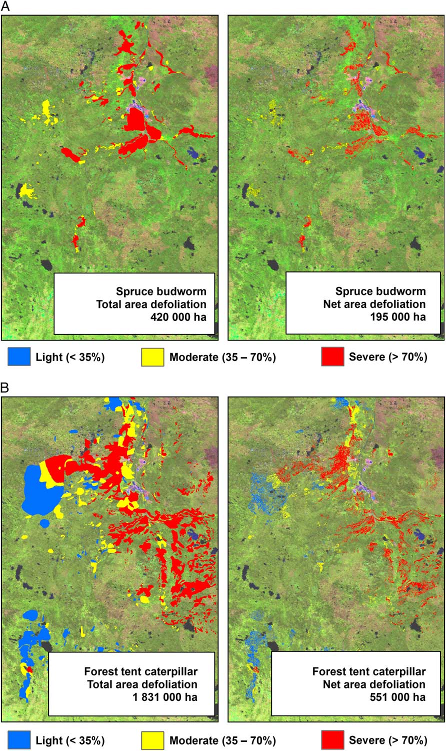
Fig. 1 Net down of aerial survey based on a GIS overlay with forest inventory polygons for damage caused by (A) spruce budworm and (B) forest tent caterpillar.
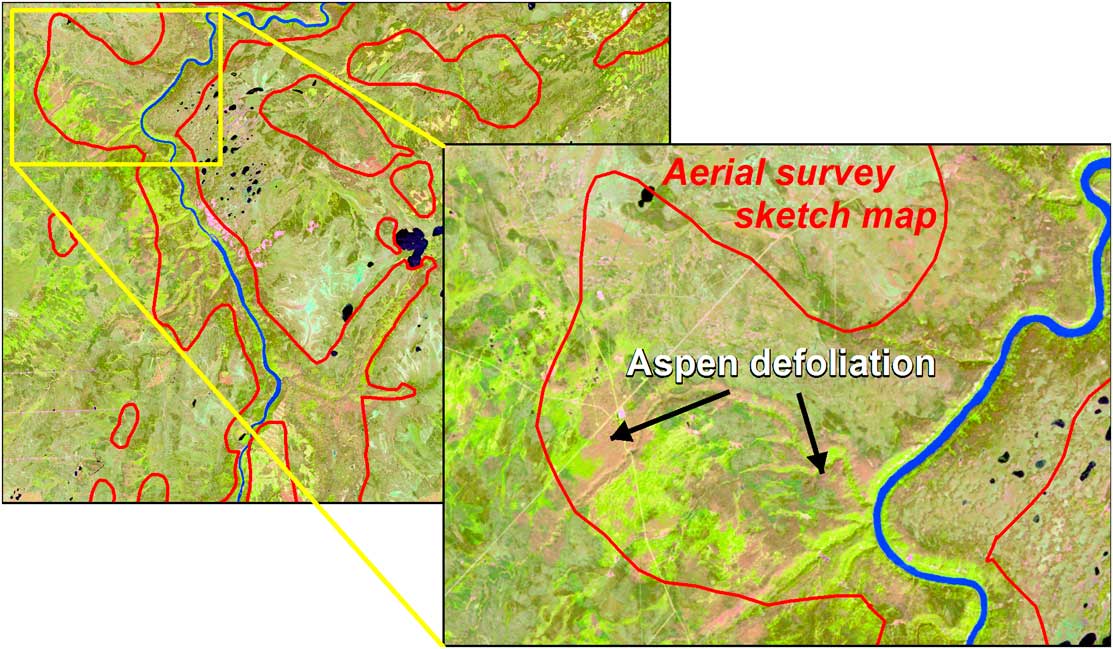
Fig. 2 Example aerial survey delineation of aspen defoliation.
Assigning a severity class can be problematic in mixed stands. Figure 3 exemplifies severe spruce budworm mortality in a mixed spruce–aspen canopy. Given that there are both living and dead trees, the general rating may warrant a “severe” class because of the conifer mortality even if not all trees have sustained damage (e.g., trembling aspen). Remote sensing would also be challenging, since the spectral response of mixed pixels will vary depending on the objects that fall within their footprint (Congalton Reference Congalton2010), which will be governed by the pixel size and the spatial distribution pattern (scattered versus clumped) of damaged trees.
Fig. 3 Example photograph of how spruce budworm defoliation creates challenges in rating damage of mixed stands when subsequently associated to a remote sensing image. Source: Alain Dupont, Société de protection des forêts contre les insectes et maladies.
There are two strategies to assessing damage using remote sensing. Many past studies have focussed on acquiring single-date or pre-outbreak and post-outbreak images from which damage is detected and assessed (Tables 4 and 5). Under this strategy, image collection needs to coincide with the dates when damage is most conducive for discriminating damage levels, which is analogous to how aerial surveys are conducted. This is a viable approach for using remote sensing to monitor specific areas (e.g., Hall et al. Reference Hall, Skakun and Arsenault2007; Townsend et al. Reference Townsend, Singh, Foster, Rehber, Kingdon and Eshleman2012), as it takes advantage of prior knowledge (e.g., past aerial surveys) to focus image acquisition, and automating the image processing can be undertaken if needed to operationalise the mapping application. Most of the studies summarised in Tables 4 and 5 employed this approach and are suited for mapping of known outbreaks or for focussed detection (e.g., where an outbreak has just started or is suspected to occur).
The second strategy is designed to detect trends over dense, long-term series of satellite imagery. It was precipitated by the free, open access data policy for Landsat data in 2008, which encouraged the development of long-term continuous monitoring for tracking land cover dynamics (Wulder et al. Reference Wulder, Masek, Cohen, Loveland and Woodcock2012a). The Landsat ecosystem disturbance adaptive processing system (LEDAPS) project, for example, created a spatially complete record of stand-clearing disturbances and recovery to study ecosystem disturbance patterns across North America (Masek et al. Reference Masek, Huang, Wolfe, Cohen, Hall and Kutler2008). LandTrendr (Landsat-based detection of trends in disturbance and recovery) was created as an approach to extract spectral trajectories of changes in land cover from annual Landsat time series (Kennedy et al. Reference Kennedy, Yang and Cohen2010). Huang et al. (Reference Huang, Goward, Masek, Thomas, Zhu and Vogelmann2010) developed a highly automated vegetation change tracker to process dense Landsat time series stacks from which disturbances such as harvest, fire, and urban development could be mapped. More recently, Hansen et al. (Reference Hansen, Potapov, Moore, Hancher, Turubanova and Tyukavina2013) produced global maps of forest depletions from 2000 to 2012 that further demonstrate the potential for automated processing of large volumes of Landsat 30-m satellite imagery. The application of these time-series approaches to pest damage assessment is a research opportunity whereby spectral trajectories could be associated to different magnitudes and types of pest damage. In addition to being suited for mapping of known outbreaks or focussed detection, it may also detect changes in imagery that may highlight new outbreaks whose locations were previously unknown.
A typical field survey averages a measure of insect damage (e.g., defoliation, mortality) within a fixed-area plot according to predefined percent intervals, and record the GPS coordinates of the plot centre (e.g., Royle and Lathrop Reference Royle and Lathrop2002; Hall et al. Reference Hall, Fernandes, Butson, Hogg, Brandt and Case2003, Reference Hall, Skakun and Arsenault2007). A problem with moving field surveys towards a more continuous scale is that in situ, visual assessment of defoliation is subjective (less so for mortality), and observer bias will depend on individual expertise (e.g., Wulff Reference Wulff2002; Mizoue and Dobbertin Reference Mizoue and Dobbertin2004). As a result, agencies employ training, periodic field calibration, and quality checks to minimise errors and to ensure consistency. Branch sample assessments such as the Fettes method (Fettes Reference Fettes1950) require more time than ocular assessments, but have resulted in higher correlations with remote sensing measures of spectral response (Hall et al. Reference Hall, Filiatrault, Deschamps and Arsenault2009). Attention to field data collection protocols is therefore a relevant component to remote sensing assessment of pest damage.
Aerial survey and remote sensing: considerations for integrated mapping and monitoring of insect damage
Aerial survey is the primary tool for mapping the location and severity of forest pest damage, and it will likely continue to be relied upon by the forest health community. These surveys are used for a wide range of purposes that aside for reporting on provincial and national pest conditions, are also used to support pest management and control efforts, forest health research and others (Westfall and Ebata Reference Westfall and Ebata2014). Aerial surveys provide input to pest management decisions and are used in both jurisdictional and national annual reporting requirements. In addition, the legacy of long-term annual surveys provides the opportunity to derive trends that reveal the coarse-scale dynamics of pest conditions.
The National Forest Pest Strategy (NFPS) was created to foster a proactive, risk-based approach to forest pest management, of which monitoring data serve as an essential foundation (Canadian Council of Forest Ministers 2012b). To realise NFPS goals, an assessment of forest health monitoring was undertaken in Canada to highlight compatibilities and differences in survey methods, and to identify monitoring gaps (Canadian Council of Forest Ministers 2012b). The problem of monitoring gaps is particularly relevant for northern latitudes, where more complete monitoring would entail costs and increases in capacity and capability beyond what is currently available (Canadian Council of Forest Ministers 2012b). In a survey of research needs, among the highly ranked topics were “spatial and temporal analysis of pest data to enable detection of changes in pest behaviour and distribution due to climate change, analysis of regional and national population trends, and quantification of losses” (Hodge Reference Hodge2014). Addressing the data gaps and these research needs, at least in part, provides a rationale for using remote sensing for forest pest monitoring.
Our review confirms that aerial survey and remote sensing maps of pest damage are not directly equivalent in terms of areas delineated. The reduction of aerial survey delineated areas through a post-GIS overlay with forest inventory or land cover data, however, is an attempt to derive a more spatially precise estimate of pest damage. While this approach is already being employed in Canada, it is not universally applied to all forest pests, nor in all provincial and territorial jurisdictions. To create a monitoring system that integrates aerial survey and remote sensing will require the harmonisation of pest damage areas between these methods, and the willingness to incorporate remote sensing to fill data gaps for achieving more complete reporting where needed.
What is the management context for forest health information within which remote sensing can help? There are four prospective roles that current data and methods could play. First, remote sensing could have a complementary role in mapping damage on an annual basis, which would require the development of a system that integrates both aerial surveys and remote sensing. Second, remote sensing could be further pursued as the vehicle to address identified data gaps (Canadian Council of Forest Ministers 2012b). Third, remote sensing could be used for special purpose studies requiring pest damage data of finer resolution for addressing questions of impact on ecology, management, and carbon. Fourth, remote sensing could support retrospective analyses and predictive modelling, such as those undertaken to estimate trends in the progression of the recent mountain pine beetle outbreak in western North America (Wulder et al. Reference Wulder, Franklin, White, Linke and Magnussen2006b, Reference Wulder, White, Grills, Nelson, Coops and Ebata2009c; Robertson et al. Reference Robertson, Nelson and Boots2007; Chen Reference Chen2014; Meddens and Hicke Reference Meddens and Hicke2014).
There are at least two factors that challenge the viability of remote sensing for providing useful pest damage information. The first factor pertains to the biological manifestation of damage, which must be sufficient for remote sensing detection. For example, detecting mountain pine beetle green attack is considered operationally infeasible (Wulder et al. Reference Wulder, White, Carroll and Coops2009b). With defoliators, the optimal timing for collection of remote sensing data when foliage loss is at its maximum can be very short (Table 1), with new and upcoming sensors expected to increase the opportunities for acquiring data (Table 2). Understanding pest biology with respect to the manifestation of damage and the timing when it is most visible is necessary because this governs what remote sensing sensors are most suitable, when data should be collected, and what analysis approach should be used. Research efforts at generating continuous time series, pixel compositing and combining data from similar sensors may help address the remote sensing viability question (Roy et al. Reference Roy, Wulder, Loveland, Woodcock, Allen and Anderson2014; White et al. Reference White, Wulder, Hobart, Luther, Hermosilla and Griffiths2014).
The second factor pertains to the information needs of forest health managers, which vary depending on the stage of the pest outbreak. In the early phases of detection, where populations are mostly endemic, remote sensing, traditionally, has not been able to play a prominent role relative to population monitoring. However population monitoring is prohibitively expensive for early detection of pest damage over large areas, particularly in remote areas where ground access is limited. Remote sensing is likely to play an increasingly important role in change detection, especially at high altitudes and latitudes, where population monitoring costs are higher and where disturbance frequencies are most likely to rise under climate change (Gray Reference Gray2013). As the outbreak progresses and peaks, there are serious limits to the accuracy of predictions derived from population models (Cooke et al. Reference Cooke, Nealis and Régnière2007), and remote sensing is likely to play an increasingly important role for continually revising forecasts, particularly those done at very large scales. As continued annual defoliation results in cumulative mortality, the forest pest manager’s context changes from pest population management to salvage logging, and the goals shift from detecting defoliation to quantifying mortality. Remote sensing products thus need to be adjusted to produce the information needed at the given phase of the outbreak. All of these potential applications are constrained by the logistics of timing, availability of resources, and data.
Future outlook
In addition to the development of integrated monitoring systems that combine aerial survey and remote sensing for mapping and monitoring forest pest damage, we speculate about how ongoing and upcoming technological advances could evolve into future remote sensing of forest pest damage. While the costs associated with these advances are always a consideration, we identified seven areas that can be grouped into analysis approaches, field measurements and sensor developments:
Analysis approaches:
-
1) Innovative time series approaches to pixel-based change detection are being developed as a result of the opening of the Landsat archive (Roy et al. Reference Roy, Wulder, Loveland, Woodcock, Allen and Anderson2014). Examples include new cloud and shadow masking methods, mosaicking, and temporal compositing approaches to generate the pixels of the highest quality for analysis (Roy et al. Reference Roy, Wulder, Loveland, Woodcock, Allen and Anderson2014; White et al. Reference White, Wulder, Hobart, Luther, Hermosilla and Griffiths2014). For example, the continuous monitoring of forest disturbance algorithm (CMFDA; Zhu et al. Reference Zhu, Woodcock and Olofsson2012) estimates sigmoidal models for each pixel and spectral band of multi-year time series of satellite multispectral observations. Once fitted for every single pixel of the area of interest, CMFDA can accurately detect any nonseasonal change that deviates from model predictions after three consecutive clear observations, which may enable the early detection and tracking of insects outbreaks as new images become available. Testing of this approach for pest damage would be necessary to verify its application potential.
-
2) Two areas in change detection research that offer potential for forest pest application include object-based change detection and data fusion from multitemporal images. Rather than using individual pixels as analysis units, object-based change detection uses image objects, that is, a group of connected pixels that are more similar between themselves than when compared with their surroundings (Chen et al. Reference Chen, Hay, Carvalho and Wulder2012). This is advantageous when the objects of interest (e.g., tree crowns) are much larger than the pixels, as is the case in imagery of submetric resolution, especially because information regarding the spatial context and mutual relations between image objects can be exploited in the analysis (Hussain et al. Reference Hussain, Chen, Cheng, Wei and Stanley2013). The second area, image fusion, involves the integration of multi-source, multi-resolution information to improve the change detection process (Zhang Reference Zhang2010; Du et al. Reference Du, Liu, Xia and Zhao2013). Given that differences in insect damage severity can be subtle, incorporating other source data that identifies the host tree species and removing other areas not relevant to forest change could improve detection and mapping of pest damage. The absence of current studies of object-based change detection and image fusion suggest its application for assessing pest damage could be an area of future research.
Field measurements:
-
3) Field methods are being subject to further automation and sophistication. Inexpensive wireless sensor networks (Chen et al. Reference Chen, Chuang and Jiang2013) are being deployed to detect and monitor insect pest infestation using a variety of sensors, from acoustic recorders to detect feeding larvae of wood-boring beetles (e.g., Chesmore and Schofield Reference Chesmore and Schofield2010) to chemiresistors that detect semiochemicals emitted by the pests or their hosts (e.g., Weerakoon et al. Reference Weerakoon, Hiremath and Chin2012). Plot-level defoliation estimates could be obtained using ground-based, zenithal digital hemispherical photography, which is customarily used to derive leaf area index and other biophysical parameters using semi-automated algorithms embedded in both commercial and free software (Chianucci and Cutini Reference Chianucci and Cutini2012); or even from photogrammetric point clouds (see 6 below) derived from hand-held cameras (Liang et al. Reference Liang, Jaakkola, Wang, Hyyppä, Honkavaara and Liu2014). Repeated photograph acquisitions in the same plots would allow an accurate estimate of defoliation (e.g., Kubo et al. Reference Kubo, Gavrilov, Muramoto and Kamata2012), and these measurements would enable a better linkage with remote sensing data.
Sensor developments:
-
4) New spaceborne sensors will augment our capacity to detect, assess, and track damage. Of particular relevance is the recent launch of the first satellite of the European Sentinel-2 constellation, which will provide, free of charge, weekly optical observations at 20-m spatial resolution (10 m for some of the spectral bands) along 290-km swaths (Drusch et al. Reference Drusch, Del Bello, Carlier, Colin, Fernandez and Gascon2012), and thus will considerably enhance the provision of high spatio-temporal resolution data for forest health monitoring. The combination of Landsat 8 and Sentinel-2, for example, results in up to eight image acquisitions within a month that greatly increases the potential for acquiring cloud-free images to track disturbances (Zhu et al. Reference Zhu, Woodcock and Olofsson2012).
-
5) There is tremendous growth in LiDAR data acquisition capabilities from ground, airborne, and spaceborne platforms (Harpold et al. Reference Harpold, Marshall, Lyon, Barnhart, Fisher and Donovan2015). Data from these sensors will require advancements in processing and analysis, linkages to in situ observations, and integration with other remote sensing data as a basis to advance applications (Harpold et al. Reference Harpold, Marshall, Lyon, Barnhart, Fisher and Donovan2015). Some of these advances, including increased data coverage and quality, as well as the use of multispectral or hyperspectral lasers with full-waveform are now in development (Hakala et al. Reference Hakala, Suomalainen, Kaasalainen and Chen2012; Harpold et al. Reference Harpold, Marshall, Lyon, Barnhart, Fisher and Donovan2015). Repeat multispectral laser scanning has the potential to monitor the changes in the structure and physiology of the tree canopy (Hakala et al. Reference Hakala, Nevalainen, Kaasalainen and Mäkipää2015) that could be applicable to measurement of insect damage if the costs associated with repeat data acquisition and processing are considered justifiable relative to the information derived. Multispectral waveform LiDAR offers a particular advantage in being able to characterise both vegetation structure and reflective properties (Hovi and Korpela Reference Hovi and Korpela2014), which would also be conducive to studies of tree and forest condition. As a result, advances in these sensors will offer increased capabilities in structural and spectral sensitivities to changes in forest foliage and biomass that will no doubt result in increased future application to assessments of forest insect damage.
-
6) There is potential to quantify defoliation using UAV photogrammetric point clouds from repeated acquisitions before, during, and after defoliation, especially for pests where the pattern of defoliation starts from the tree tops and outside of tree crowns inwards such as spruce budworm and jack pine budworm. These point clouds are a sort of three-dimensional model of the canopy; can be derived from overlapping photographs taken from consumer-grade cameras using the “structure from motion” computer vision approach (Snavely et al. Reference Snavely, Seitz and Szeliski2008); and have a much lower cost in data acquisition and processing than LiDAR point clouds. They could be a suitable substitute when the focus is on the outer envelope of the forest canopy, which is where the majority of points from these clouds are located (White et al. Reference White, Wulder, Hobart, Luther, Hermosilla and Griffiths2014). Future UAV systems will be designed to make autonomous decisions regarding where and how they should fly to complete a preprogrammed task, and how they can complete the task most efficiently. Hence they will augment the capacity of the field crews to expediently collect data to calibrate and validate aerial surveys and remote sensing-based assessments of pest condition.
-
7) We anticipate that new synergies will evolve from the integration of technologies. UAVs will carry LiDAR and hyperspectral sensors (e.g., Wallace et al. Reference Wallace, Lucieer, Watson and Turner2012; Zarco-Tejada et al. Reference Zarco-Tejada, González-Dugo and Berni2012) that will improve measurements of canopy condition that could then be associated with pest damage. New smartphone applications that take advantage of the phone’s GPS, camera, and microphone capacities will change the efficiency and mechanism with how data capture will be undertaken and this is anticipated to change the collection of biological data and potentially reduce the cost of monitoring programmes (August et al. Reference August, Harvey, Lightfoot, Kilbey, Papadopoulos and Jepson2015). Integrated information systems (e.g., Fang et al. Reference Fang, Da Xu, Zhu, Ahati, Pei and Yan2014) that combine data from disparate sources, communicate and act upon the sensors through the Internet (Gubbi et al. Reference Gubbi, Buyya, Marusic and Palaniswami2013), and share data and analytics through the Internet will expand both the way insect pests are monitored and our knowledge about them.
Summary of lessons learnt
Aerial survey is the dominant tool for monitoring insect disturbances, because it is relatively cost effective in meeting a specific client need. It has provided a long-term legacy of forest health information in Canada and is likely to continue into the foreseeable future. There is a growing demand, however, for pest information of lower cost, greater extent and increased precision in terms of delineation and severity (Bernier et al. Reference Bernier, Kurz, Lemprière and Ste-Marie2012). Remote sensing is a potential solution to address these demands, resolve data gaps and augment aerial surveys by increasing the precision and detail of the information in an integrated forest pest monitoring system. The multitude of remote sensing studies and our direct experience provides several lessons that could help focus how the integration of remote sensing into a pest monitoring system could be achieved. The summary of lessons learned and recommendations include:
-
1) Fundamental to the detection of damage is understanding how damage manifests, when will it be visible, and at what spatial scale. Since this varies by pest, detection requires knowledge of the pest–host–image triangle. For example, forest tent caterpillar damage is characterised as foliage loss that is only detectable in remote sensing image acquisitions for a limited time because of the ability of trembling aspen to re-flush following defoliation.
-
2) Aerial surveys and remote sensing maps of pest damage are not necessarily substitutable but they are complementary. Some provincial jurisdictions, in a movement towards more closely approximating net areas of impact, are overlaying aerial survey maps with forest inventory data to remove non-susceptible forest types. While this approach improves the aerial survey, it is still based on the assumption that all areas within a susceptible forest type suffered the same level of damage assigned in the aerial survey polygon. Remote sensing would further refine these areas by only mapping damage where it occurred and by providing more precise estimates of severity.
-
3) The discrete severity classes used in aerial or field surveys, while relevant for operational monitoring and reporting needs, are limiting when used as reference data for calibration against continuous spectral data from remote sensing imagery. Since field information is necessary to anchor remote sensing assessments and for validation, capturing severity data on a more continuous scale is encouraged. Greater attention to field data collection protocols, including controlling for subjectivity, is necessary for deriving valid remote sensing assessments.
-
4) Mixedwood stands are challenging to assess because a given defoliator will typically only attack a particular host tree species. That host tree species may also be unevenly distributed within the stand, and this results in mixed pixels that contain both non-susceptible and susceptible trees, where the latter may have sustained different levels of damage. Addressing this problem requires methods and models specific to mixedwood stands from which to calibrate remote sensing spectral response to damage.
-
5) Defining the information need according to spatial extent will help to determine which of two strategies to implement when using remote sensing to assess pest damage. The first strategy employs image pairs, typically two images representing pre-outbreak and post-outbreak, from which changes are detected, or in some cases a single date image depending upon the clarity of the pest damage pattern. While this strategy is viable for monitoring specific areas, an alternative is emerging based on time series analysis of image stacks from multiple dates where the temporal profile of individual pixels is extracted and analysed. The second strategy is based on the increasing availability of freely available data from more satellites than just Landsat. This enables the concept of a continuous time series approach with pixel substitution strategies to generate cloud free mosaics that promises to dispel the difficulty of acquiring image data at the time when the application warrants (White et al. Reference White, Wulder, Hobart, Luther, Hermosilla and Griffiths2014). Regardless of strategy, there is a need to translate pixel change to changes in pest damage that are useful for a forest health manager.
-
6) There are four roles that remote sensing could serve in a management context: contributing to annual mapping; filling data gaps; providing data for special purpose studies of pest impacts; and supporting both retrospective analyses and predictive modeling. As with any tool, there are practical realities that limit when remote sensing is a viable solution; understanding these is a prerequisite for successful application. Integrating remote sensing into forest health monitoring programmes will help to address the increasing demand to map and monitor at finer levels of both spatial detail and magnitude of damage.
A list of new innovations underway in the field of remote sensing was presented, from which we speculated about what these advances may offer to future forest health assessment. New technologies regarding satellite sensors, airborne LiDAR, UAV, and methods of analysis will no doubt play a role in future forest health monitoring programmes. While much of the knowledge and tools to develop a more integrated pest monitoring system are available today, technological innovation will continue to push the limits of what we can do tomorrow.
Acknowledgements
Some of the foundation of this review paper was developed in collaboration with the Canada Centre for Remote Sensing (CCRS) as part of a Government Related Initiatives Program project funded by the Canadian Space Agency (CSA) under the management of Paul Briand entitled “Gauging the health of Canada’s forests: accounting for insect defoliation and dieback in the indicators of sustainability for Canadians”. Contributors to that project included Sylvia Thomas (co-principal investigator with R. Hall), Joost van der Sanden, Alice Deschamps, Robert Landry, and Lori White from CCRS. Other contributors from the Canadian Forest Service included Eric Arsenault (now with CSA) and Michelle Filiatrault. Michelle and Sebastien Rodrigue are acknowledged for assistance in assembling and checking the references of an earlier version. Review comments by Dave Langor and Janice Hodge of an earlier version of the paper and journal reviews provided by Don Leckie and Ken Raffa helped to significantly improve the manuscript and are greatly appreciated.