


1. Introduction
Functional mapping has proven to be a powerful approach for mapping quantitative trait loci (QTLs) responsible for dynamic traits whose phenotypic values change with time or other independent variables (Ma et al., Reference Ma, Casella and Wu2002; Wu et al., Reference Wu, Ma, Lin and Casella2004a, Reference Wu, Ma, Lin, Wang and Casellab, Reference Wu, Wang, Zhao and Cheverudc; reviewed in Wu & Lin, Reference Wu and Lin2006). A general strategy for QTL mapping is to construct a finite mixture model (Lander & Botstein, Reference Lander and Botstein1989; Jansen & Stam, Reference Jansen and Stam1994; Zeng, Reference Zeng1994) in which any individual from a mapping population is assumed to arise from one of the multiple possible QTL genotypes. For a quantitatively inherited trait, each group of QTL genotypes is thought to follow a normal distribution with a mean expressed as the genotypic value and a variance common to each group. The central idea of functional mapping is that the mean vectors of QTL genotypes in a time limit are modelled by a biologically meaningful mathematical equation, whereas the covariance matrix is modelled in terms of its time-series autocorrelation structure (Ma et al., Reference Ma, Casella and Wu2002).
From a biological viewpoint, functional mapping is advantageous because it incorporates fundamental principles behind biological processes or networks into a QTL mapping framework. Much attempt has been made to embed various mathematical and differential equations in the mapping framework to reveal dynamic changes of genetic control over a biological or medical trait given its developmental nature. For example, the Richards growth equation has been used to model growth trajectories for various biological entities, bi-exponential curves to approximate HIV-1 dynamics (Perelson et al., Reference Perelson, Neumann, Markowitz, Leonard and Ho1996), Emax models to fit drug response curve over a range of concentrations (Giraldo, Reference Giraldo2003) and power curve to quantify the power required for a bird to fly at a particular speed (Tobalske et al., Reference Tobalske, Hedrick, Dial and Biewener2003). The parameters in these equations have particular biological or clinical means. Thus, the results from functional mapping are biologically more interpretable and relevant than those from general approaches without biological incorporation. Also, through testing, individually or in combination, for the curves parameters in functional mapping, many biologically interesting questions can be asked and addressed at the interplay between genetic actions and developmental patterns (Wu et al., Reference Wu, Ma, Lin and Casella2004a).
Functional mapping attempts to estimate mathematical parameters that model the time-dependent vector of QTL effects and residual covariance matrix rather than estimate all elements in the vector and matrix and, therefore, displays strong statistical robustness due to the estimation of fewer parameters (Ma et al., Reference Ma, Casella and Wu2002). In previous functional mapping, approaches for modelling the structure of the covariance matrix include the autoregressive (AR) (Diggle et al., Reference Diggle, Heagerty, Liang and Zeger2002) and structured antedependence (SAD) model (Núñez-Antón & Zimmerman, Reference Núñez-Antón and Zimmerman2000). Whereas the AR model assumes variance stationarity and correlation stationarity, these two assumptions are relaxed for the SAD model that approximates the variance and correlation as a function of time. Zhao et al. (Reference Zhao, Chen, Casella, Cheverud and Wu2005) found that the AR and SAD models cannot be replaced by each other, although the SAD model seems to be more general in terms of its non-stationary nature. In statistical modelling of longitudinal variables, many other models have been available to structure the covariance matrix, all of which can be potentially used for functional mapping. Thus far, a comprehensive treatment of modelling the covariance matrix has not been fully explored. Meyer (Reference Meyer2001) systematically reviewed various approaches for estimating covariance functions related to cattle genetic and breeding studies. The purpose of this study is to incorporate several most commonly used covariance-structuring approaches into the framework of functional mapping, aimed at providing a general strategy for the choice of an optimal approach for structuring the covariance matrix for practical data sets.
2. Model and method
(i) Genetic model
We start with a simple F 2 population from two homozygous lines. Consider one segregating QTL, with three genotypes, QQ (2), Qq (1) and qq (0), responsible for dynamic changes of a trait. All n progeny in the pedigree are measured for the dynamic trait at each of T time points. The trait phenotype (yi) of progeny i measured at time t can be expressed as
where ξ ij is an indicator variable describing a possible genotype j(j=2,1,0) of the QTL for progeny i and defined as 1 if a particular genotype is observed and 0 otherwise, μ j(t) is the genotypic value of the trait for QTL genotype j at time t, and ei(t) is the residual including the aggregate effect of polygenes and error effect and distributed as N(0, σ2(t)). The covariance between residuals at two different time points, t 1 and t 2, is expressed as σ(t 1, t 2). The variances and covariances form a residual covariance matrix Σ. The probability of ξ ij to take 1 or 0 can be inferred from the two-locus genotypes of the fianking markers that bracket the QTL, expressed as the conditional probability of the QTL genotype given marker genotypes described in terms of the recombination fractions between the QTL and the two markers.
(ii) Likelihood function
The likelihood of the dynamic trait with T-dimensional measurements yi=(yi(1), …, yi(T)), and marker data, M, can be represented by a multivariate mixture model
where the mixture proportion, ![]() , is the conditional probability of QTL genotype given a marker genotype for progeny i, which describes the position of the QTL (θ) within the marker interval, and fj(yi) is the multivariate normal density with mean vector uj=(μ
j(1), …, μ
j(T)) and variance matrix Σ.
, is the conditional probability of QTL genotype given a marker genotype for progeny i, which describes the position of the QTL (θ) within the marker interval, and fj(yi) is the multivariate normal density with mean vector uj=(μ
j(1), …, μ
j(T)) and variance matrix Σ.
Several numerical methods can be used to solve the maximum likelihood estimates (MLEs) of the parameters (θ, uj, Σ) that define the likelihood function (2). Like a general treatment, functional mapping estimates θ with a grid approach, i.e., the likelihood values are plotted against the length of a linkage group and the peak of the likelihood profile is then regarded as the location of QTL. However, functional mapping attempts to estimate and test the parameters that model the structures of (uj, Σ), instead of estimating all the elements contained within (uj, Σ). The parameter vectors for modelling the mean vector and covariance matrix are denoted as ![]() for QTL genotype j and Ω
v, respectively.
for QTL genotype j and Ω
v, respectively.
(iii) Submodel for structuring the mean vector
If the traits studied follow a certain pattern of development, mathematical equations can be used to model the mean vector. For example, growth trajectories for biological entities at different organizational levels can be approximated by the Richards growth equation. The power required for a bird to fly at a particular speed can be identified by incorporating power curves. Bi-exponential curves and Emax models have been utilized to approximate HIV-1 dynamics after drug treatment and drug response at different concentrations, respectively. In general, the time-dependent mean vector of a dynamic trait is described by a mathematical function
where ![]() is a set of curve parameters that define the dynamic mechanism of a particular trait.
is a set of curve parameters that define the dynamic mechanism of a particular trait.
In practice, many dynamic traits may not be described by a mechanistic model, relying on statistical fitting. Functional mapping for these kinds of traits can be based on non-parametric modelling. Statistically, many non-parametric approaches have been available; for example, B-spline, P-spline or orthogonal polynomials.
(iv) Submodel for structuring the covariance matrix
An unstructured matrix would be best to fit the residual covariance since it can approximate the true structure, but with the measured time points increased, the unstructured matrix is too large to be solved. The structured models with more parameters are more appropriate than fewer ones, but the number of parameters in structured models is more, and the structured models is more closed to unstructured ones. So, the covariance matrix Σ should be structured to consider the inherent pattern of time-dependent variances and covariances, reduce the number of unknown parameters being estimated and decrease the effect of noises on the precision of QTL mapping. The simplest approach for structuring the matrix is based on the AR model, in which the variance and covariance assumes the stationarity, i.e. there is the same residual variance for the trait at each time point and the covariance between different measurements decays purely with time interval. The variance stationarity assumption has been relaxed by implementing the transform-both-sides (TBS) model (Carroll & Puppert, Reference Carroll and Puppert1984) within the context of functional mapping (Wu et al., Reference Wu, Ma, Lin, Wang and Casella2004b). The SAD model was used to characterize the non-stationary variance and correlation (Núñez-Antón & Zimmerman, Reference Núñez-Antón and Zimmerman2000).
However, the AR and SAD models can be only used in their respective situations. The residual variances and covariances characterized by both the models include contributions by other QTLs and errors. Because the residual may also change with time interval in a particular manner, the AR and SAD models will display different powers to detect QTL. Here, we propose a general model for structuring the residual covariance matrix, which covers the features of the AR and SAD models.
According to the theory of matrix algebra, we can decompose Σ into the product of standard deviations and correlations expressed as
where V 1/2 is the diagonal matrix that is composed of the residual standard deviation σ(t) for t=1, 2, …, T, and R is the correlation matrix. Approaches have been available to model the structures of V and R.
(a) Standard deviation function
A number of variance functions have been proposed to model heterogeneous variances across different time points (Foulley et al., Reference Foulley, Quaas and D'Arnoldi1998). These functions include a step function or a polynomial function as follows:

where σ2 is the variance at the intercept, br is the coefficient of the variance function and v is the order of polynomial fit. The standard deviation function is the square root of σ2(t).
(b) Correlation function
Correlations in R between different time points can be modelled as a function of time interval. Correlation functions with one or more parameters can be either stationary or non-stationary model without variance. The simplest correlation function is those specified by a single parameter. Table 1 lists several stationary models for correlation functions with a single parameter. Equation (4) can be reduced to the first-order AR (AR(1)) covariance structure when σ2(t) is equal to σ2 and when the correlation function is specified by the AR(1) model. All the parameters that describe the standard deviation and correlation functions are arrayed in Ω v.
Table 1. Common stationary models for correlation functions with a single parameter
Note: l denotes the lag in time for a pair of time points.
More complicated models, such as autoregressive moving average (ARMA), can be considered to model correlation functions. The ARMA model typically contains two parts, an AR and a moving average (MA). The model is usually referred to as an ARMA (p, q) model, where p is the order of the AR part and q is the order of the MA part. For some data, non-stationary models perform better than stationary models in the functional mapping (Zhao et al., Reference Zhao, Chen, Casella, Cheverud and Wu2005; Lin & Wu, Reference Lin and Wu2006; Cui et al., Reference Cui, Wu, Casella and Zhu2008). The SAD model is one class of non-stationary models (Zimmerman & Núñez-Antón, Reference Zimmerman and Núñez-Antón2001). The form of the SAD model was described in Zhao et al. (Reference Zhao, Chen, Casella, Cheverud and Wu2005) who provided a closed form of the SAD-structured covariance matrix.
(v) Hypothesis tests
Whether there is a significant QTL that controls the developmental process of a dynamic trait should be tested by calculating the likelihood ratio statistic, expressed as
where ![]() and
and ![]() are the MLEs of the curve parameters and the parameters that structure the residual variance matrix under the null hypothesis (there is no QTL) and
are the MLEs of the curve parameters and the parameters that structure the residual variance matrix under the null hypothesis (there is no QTL) and ![]() ,
, ![]() and
and ![]() are the MLEs of the QTL position, genotype-specific curve parameters and matrix-structuring parameters under the alternative hypothesis (there is a QTL), respectively.
are the MLEs of the QTL position, genotype-specific curve parameters and matrix-structuring parameters under the alternative hypothesis (there is a QTL), respectively.
The plug-in LR value calculated by eqn (6) follows asymptotically a chi-square distribution with degrees of freedoms equal to the difference in the numbers of parameters between the models with the two different hypotheses. The critical threshold for claiming the existence of a QTL can be empirically determined on the basis of permutation tests.
Functional mapping allows for the test of various biologically relevant hypotheses regarding the genetic control of developmental timing. Wu et al. (Reference Wu, Ma, Lin and Casella2004a) formulated a number of such hypotheses and applied them to a practical example in poplar trees.
(vi) Model selection
For a practical data set, we should know which model is optimal to explain the structure of the covariance matrix. The selection of an optimal covariance-structuring model is crucial for increasing the power of functional mapping and its estimation precision. In statistics, there are several criteria for model selection although none of them perform the best under all circumstances. Here, we used the commonly used Bayesian information criterion (BIC) (Schwarz, Reference Schwarz1978) as the model selection criterion of the optimal combination of two submodels with parsimonious parameters. The BIC is defined as
where ![]() and
and ![]() are the MLEs of parameters under a particular model (M),
are the MLEs of parameters under a particular model (M), ![]() ) represents the number of independent parameters under this model and n is the total number of observations on all individuals. The optimal model is the one that displays the minimum BIC value.
) represents the number of independent parameters under this model and n is the total number of observations on all individuals. The optimal model is the one that displays the minimum BIC value.
3. Results
A doubled-haploid (DH) population with 111 lines was generated by crossing an indica rice variety Gui-630 and a japonica rice variety Taiwanjing (Weng et al., Reference Weng, Wu, Li, Liu, Tang, Zhou and Zhang2000). A linkage map composed of 175 RFLP markers was constructed for the DH population, covering a total length of 1225 cM. This DH population was grown with replicates in a field trial (Zhou et al., Reference Zhou, Li, Wu, Chen, Mao and Worland2001). For each plant, the number of developed leaves on the main stem was counted, and the length of the developing leaf was measured every 5–7 days from day 30 after sowing until the full development of the leaf. These measured data were used to estimate the leaf age of a plant (y) using

The growth of leaf age of a plant can be fit by a mathematical equation. We will use three equations to model leaf age growth which include:
(1) Richards' (RIC) model expressed as
(2) A power curve (POW) expressed as
(3) A parabolic curve (PAR) expressed as
where the parameters a, b, c and/or d in the three above equations can be explained in a biological sense. By estimating these parameters and testing their differences among different QTL genotypes, we can determine whether and how a QTL triggers an effect on leaf age growth trajectories.
Considering the data of leaf age growth may not follow any curve, we use a non-parametric approach based on Legendre (LEG) polynomials (Meyer, Reference Meyer2001; Yang et al., Reference Yang, Tian and Xu2006) to approximate the dynamic change of leaf age in development. In this study, the Legendre polynomial of order 2 is considered and expressed as
where ![]()
These parametric and non-parametric approaches are incorporated into the framework of functional mapping, along with modelling the structure of the covariance matrix by the standard deviation function, ![]() with different orders (see eqn (5)), and the correlation function (Table 1). All possible combinations between standard deviation functions and correlation functions are each incorporated into functional mapping. By calculating the BIC values, an optimal combination can be determined. Table 2 tabulates the BIC values for each combination of standard deviation and correlation functions under different submodels of the mean vector. It can be seen that different combinations give markedly different BIC values. In general, the Gaussian model of the correlation function performs best among all the models, followed by the uniform distribution model. Combing the Gaussian model and the standard deviation function of order 1 with the power curve for the mean vector provides an optimal fit of the data (Table 2).
with different orders (see eqn (5)), and the correlation function (Table 1). All possible combinations between standard deviation functions and correlation functions are each incorporated into functional mapping. By calculating the BIC values, an optimal combination can be determined. Table 2 tabulates the BIC values for each combination of standard deviation and correlation functions under different submodels of the mean vector. It can be seen that different combinations give markedly different BIC values. In general, the Gaussian model of the correlation function performs best among all the models, followed by the uniform distribution model. Combing the Gaussian model and the standard deviation function of order 1 with the power curve for the mean vector provides an optimal fit of the data (Table 2).
Table 2. BIC information criteria for leaf age data from different combinations of sub-models
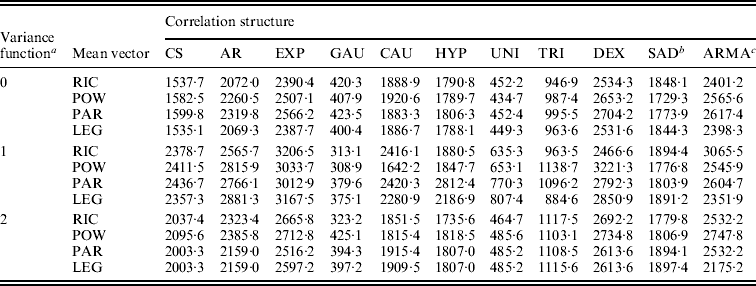
a The variance structure is modelled by a power equation of different orders 0–2.
b SAD is specified as the first-order SAD model.
c ARMA is specified as the autoregressive moving average model with the first-order AR part and the first-order MA part.
Table 3. The MLEs of the model parameters and their asymptotic standard errors in the parentheses under the combination of POW and GAU distribution models for leaf age growth trajectories
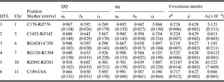
Figure 1 gives the profile of LR test statistics across all the 12 chromosomes under the optimal combination. Permutation tests based on 1000 replicates have been used to determine the genome-wide empirical critical threshold for significance declaration. There are a total of six peaks for the LR profile that surpass the threshold, suggesting the detection of QTL for leaf age growth. These QTLs are located on different chromosomes 1, 2, 6, 7, 10 and 11, respectively (Fig. 1). Table 3 tabulates the estimates of the curve parameters for each QTL genotype and the parameters that model the structure of the covariance matrix. As shown by the estimates of the standard errors obtained with the bootstrapping approach, the parameter estimation has reasonably high precision. Using the estimated curve parameters, two curves for leaf age growth are drawn for each QTL genotype (Fig. 2). Based on the differences in curve shape between the two QTL genotypes, all the six QTLs detected display a substantial effect on leaf age growth during the entire development of plants.
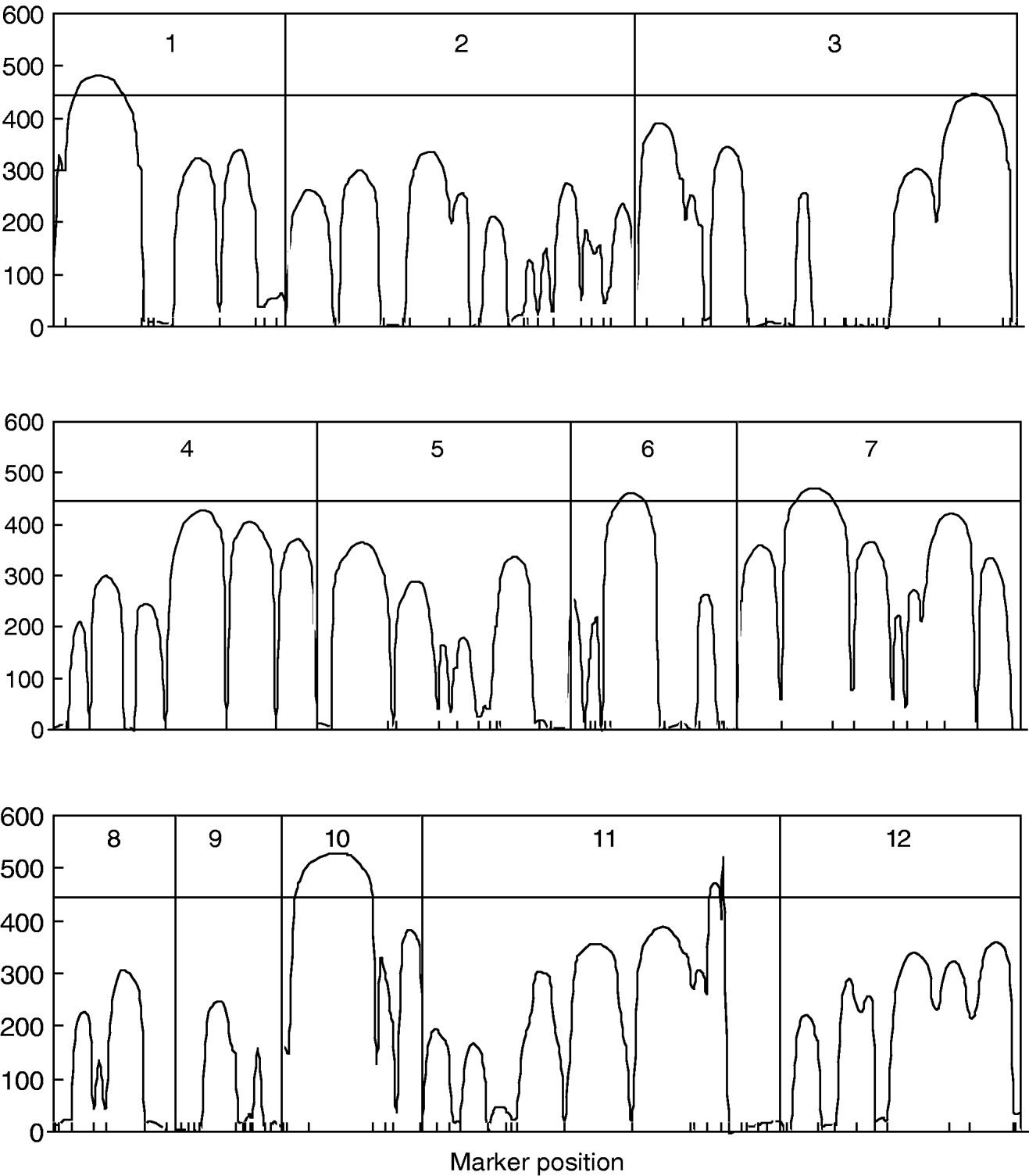
Fig. 1. The profile of the log-likelihood ratios between the full and reduced (no QTL) model for leaf age growth trajectories across the genome. The genome-wide threshold value is given as a horizontal line. Ticks indicate the positions of markers on linkage groups.
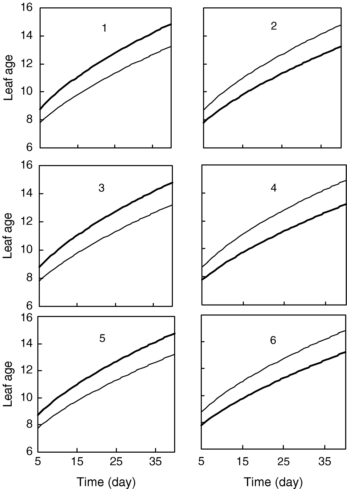
Fig. 2. Two growth curves each presenting two groups of genotypes (bold lines are for QQ) at the six QTLs, symbolized by 1, 2, …, 6, detected on chromosome 1, 3, 6, 7, 10 and 11, respectively.
4. Discussion
Functional mapping incorporates fundamental principles behind biological processes or networks that are bridged with mathematical functions into a QTL mapping framework (Ma et al., Reference Ma, Casella and Wu2002; Wu & Lin, Reference Lin and Wu2006). Functional mapping involves not only modelling time-dependent expected mean vectors of QTL genotypes but also the structure of the within-subject residual covariance matrix. The mean vectors of QTL genotypes were usually modelled by biological meaningful functions including a few key parameters that define the shape and function of a particular biological network (see also Wu et al., Reference Wu, Zhou, Li, Mao and Chen2002). Because of this implementation with biological principles, functional mapping provides more sensible and interpretable results than previous QTL mapping approaches (Wu & Lin, Reference Lin and Wu2006).
Functional mapping is also advantageous in statistics because the structure, rather than all the elements, of the mean vector and the covariance matrix is estimated, which can largely reduce the number of parameters to be estimated. Original functional mapping capitalizes on a simple statistical process, such as the AR process, to model the covariance structure (Ma et al., Reference Ma, Casella and Wu2002). In subsequent modelling, several more complicated processes, such as SAD, have been implemented, leading to significant results for QTL detection (Zhao et al., Reference Zhao, Chen, Casella, Cheverud and Wu2005). However, there are a number of other statistical processes (see Henderson, Reference Henderson1982; Jaffrezic & Pletcher, Reference Jaffrezic and Pletcher2000; Meyer, Reference Meyer2001) that may better suit functional mapping than the AR or SAD models given a particular data set. In this article, we implement a comprehensive set of statistical models for the structure of the covariance matrix, provide a systematic procedure for selecting an optimal approach for the mean-covariance structure, and then exemplify the utility of our model selection idea using a real example from the rice genetic mapping project (Weng et al., Reference Weng, Wu, Li, Liu, Tang, Zhou and Zhang2000; Zhou et al., Reference Zhou, Li, Wu, Chen, Mao and Worland2001).
Our implementation includes the modelling of the covariance matrix with parametric or parametric variance and correlation functions. Depending on the complexity of a problem, parametric functions may be specified by one single or more parameters, or can be stationary and non-stationary. In some situations, no parametric functions are available to capture the pattern of the covariance matrix, in which we use non-parametric modelling based on the Legendre polynomial to fit changes of the variances and covariances (Gao & Yang, Reference Gao and Yang2006; Yang et al., Reference Yang, Tian and Xu2006). Incorporated into a random regression model (Kirkpatrick et al., Reference Kirkpatrick, Hill and Thompson1994; Meyer, Reference Meyer2001), the Legendre polynomial displays the changes of the covariance matrix in a linear way, thus largely facilitating the result interpretation and computation of functional mapping. In a data analysis using a published example for leaf age growth in rice, all possible combinations of the submodels for the mean vector and covariance matrix have been considered. An optimal combination based on the model selection criterion, BIC, was determined, which includes the Gaussian model for the correlation structure, the power equation of order 1 for the variance structure and power curve for the mean vector (Table 2). Although the result was not shown in Table 2, such a combination is in fact better than the fitting of the covariance matrix with the Legendre polynomial for this particular example. For example, the Legendre polynomial of the best order 2 gives the BIC values of 2227 to 2491.
The model framework proposed in this article will provide a powerful tool for functional mapping of QTL that determine the developmental pattern of dynamic traits. The framework allows for the choice of the best fitness of the mean-covariance structure for a particular data. With this framework, we are in an excellent position to study and map the detailed genetic architecture of complex traits that undergo developmental changes in an organism's lifetime.
The preparation of this manuscript was partially supported by NSF grant (No. 0540745) and the National Natural Science Foundation of China (No. 30972077).


