


Our forecast, published in the UK chapter of this Review, is conditioned on the assumption that the result of the 23 June referendum is a vote to remain in the EU. The discussion of the economic impact in the first half of the year, and the accompanying uncertainty due to the very act of having the vote, is discussed in the UK chapter in this Review.
However, there exists a significant possibility of a vote to leave the EU. The future is, by definition, uncertain and we normally represent this with a distribution of potential outcomes around our modal path for the economy. The referendum presents a particular instance where the future may be genuinely considered bi-modal, with two distinct paths. The outcome of the referendum will determine which of these future paths the UK economy takes.
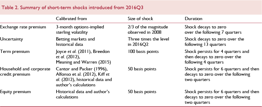
This note presents a simulation exercise designed to give a counterfactual of a world in which the UK votes to leave the EU. We discuss the short-run developments that are most likely to affect the UK economy in the immediate aftermath of a leave vote. We do this by introducing a range of shocks to our global econometric model designed to capture the effects of the UK leaving the EU. These shocks are layered together with a series of more long-run structural changes which are discussed by Ebell and Warren, in this Review.
Focusing on the near-term implications, our analysis suggests that the level of GDP in 2017 will be 1 per cent lower than our baseline forecast presented in the UK section of this Review. By 2018 this loss of output widens to 2.3 per cent. Heightened risk and uncertainty will cause sterling to depreciate by around 20 per cent immediately following the referendum, which will result in an intense bout of inflationary pressure. Meanwhile, the same uncertainty induces a tightening of credit conditions and a fall in domestic demand as consumption and investment fall relative to the counterfactual of a vote to remain.
We begin by detailing the process by which the UK would negotiate exiting the EU followed by a comprehensive exposition of the shocks that form the core of our short-run analysis. We then conclude with the quantitative implications of our simulation exercise, macroeconomic policy responses and a discussion of the transition to the longer run, which is discussed in detail in Ebell and Warren, in this Review.
The exit process
Should the vote in June result in a decision to leave the European Union, a number of things will happen. First, the UK government will notify the European Council of its intention to withdraw. The process for withdrawal is then governed by Article 50 of the Lisbon Treaty. The UK has a 2-year window to negotiate a withdrawal agreement, which would include the terms of the UK's future relationship with the EU, and which must be approved by a simple majority of the European Parliament and an enhanced qualified majority (20 out of 27) of the remaining Member States. An extension to the 2-year window can only be granted by unanimous agreement of the remaining Member States.
If the 2-year deadline is reached without an approved agreement and no extension is granted, the UK will fall back on WTO rules and so face tariffs on exports to the EU at Most Favoured Nation (MFN) rates.
During the 2-year negotiation period there will be significant uncertainty about the nature of the UK's future trading relationships with the EU and third party countries. The likely length of the negotiation process is itself uncertain as no country has previously used Article 50 to withdraw from the Union. However, we expect the 2-year timeframe to be optimistic based on previous experiences of free trade agreements. Negotiations of the Free Trade Agreement (FTA) between the EU and Canada began in 2009 and are still ongoing. Greenland's withdrawal from the European Economic Community in 1985 (predating the Lisbon Treaty, and therefore not covered by Article 50) took three years to negotiate. Negotiations will be more prolonged if the UK seeks ambitious concessions in preferential access to the Single Market, for example free trade in services. An agreement that included areas of foreign policy would require the unanimous agreement of all 27 Member States, which in some cases would require ratification by their national parliaments, significantly lengthening the process. The UK will also need to negotiate new free trade agreements with third party countries such as the US, which are likely to begin only after the agreement with the EU is finalised. Businesses which rely on non-EU trade may therefore face a lengthier period of uncertainty.
The short-run impact
A vote to leave would represent a substantial shock to the UK economy which will have consequences for the short-run outlook. To think about these consequences in the context of our econometric model (see Appendix A for a brief summary of the model) we identify and calibrate a number of more specific shocks. In the analysis presented below we first provide a discussion of these shocks as well as their calibrations. We then discuss how the imposition of these shocks changes the outlook for the UK economy compared to the path laid out in our baseline forecast presented in the earlier UK chapter.
The shocks
Exchange rate
As discussed in the UK chapter of this Review, markets have already begun to price in a period of heightened sterling volatility around the time of the referendum. Our analysis seems to indicate that this was the dominant driver of the depreciation of sterling from the start of the year to mid-April. More recently, sterling has recovered some of this ground, and market measures of uncertainty around sterling have also reduced. Looking to betting markets and other poll evidence, this reduction in risk is highly correlated with a lower weight being placed on the possibility of a vote to leave the EU. Should such a result become more likely, then we would expect to see the risk premium open up again and sterling depreciate further.
It is therefore highly likely that a vote to leave the EU on 23 June will widen the risk premium associated with sterling. The question for our analysis is, by how much? To calibrate our shock, we look to the options-implied 3-month sterling volatility. This series rose sharply on the day that the 3-month contract first encompassed the date of the referendum, and remains elevated. Comparing this increase with that observed in the recent global financial crisis we observe that it has been approximately two-thirds of the size, figure 1. We therefore calibrate a shock to the exchange rate risk premium by scaling the change in the risk premium in the fourth quarter of 2008 by two-thirds. The shock then decays by 50 per cent a quarter. It reaches zero by the end of 2017 so that by the time the negotiating window has been concluded the sterling risk premium has returned to its baseline level.

Figure 1. Option-implied 3–month sterling volatility
Uncertainty
A brief overview of the literature
Before presenting our approach to deal with the increase in uncertainty that the referendum will generate in the event of a leave vote, it is convenient to present the main results that the theoretical and empirical literature has produced on the effects of uncertainty on economic activity, as well as the different measures of uncertainty that have been developed. We cannot hope to provide a comprehensive survey in this note but at least we can highlight the main points.
A large body of literature has looked into the effects of uncertainty on investment decisions of firms. An early strand of the literature captured in the work by Reference OiOi (1961), Reference HartmanHartman (1972) and Reference AbelAbel (1983) suggested that, contrary to common belief, uncertainty could lead to higher investment if marginal returns to investment were convex. Later on, Reference BernankeBernanke (1983), Reference PindyckPindyck (1988) and Reference DixitDixit (1989) showed that under the presence of sunk costs to investment, which render marginal returns to capital concave, a firm will delay investment projects following an increase in uncertainty as there will be a value in waiting.Footnote 1 Investing triggers a cost that cannot be recovered and therefore it is optimal for the firm to wait until the realisation of the uncertain outcome ensures sufficiently high expected returns. Reference Leahy and WhitedLeahy and Whited (1996), using firm-level data, found empirical evidence of uncertainty exerting a negative influence on investment, thus giving support to the latter strand of work. Recent work includes Reference BloomBloom (2009), who finds that higher uncertainty causes firms to delay investment and hiring as well as declines in productivity growth as the rate of reallocation of resources from low to high productivity firms is inhibited, Reference Bloom, Floetotto, Jaimovich, Saporta Eksten and TerryBloom et al. (2014), who find similar results within the context of a DSGE model extended to include uncertainty shocks, and Férnandez-Villaverde et al. (2015), who find that volatility in fiscal shocks also induces negative effects on economic activity within a New Keynesian model framework. There seems to be a consensus that uncertainty drives firms to delay their investment plans.
Besides theoretical work, there has been a considerable amount of empirical work to establish a link between uncertainty and economic activity. The results have been broadly in line with the lessons we learned from the theory. Reference Beaulieu, Cosset and EssaddamBeaulieu et al. (2005) analysed four major events between 1990 and 1996, including the second referendum on the question of Quebec's independence from Canada in 1995, and found that firms with higher exposure to political risk had to generate a higher return in the period of heightened uncertainty in the run-up to the referendum. Reference DurnevDurnev (2010) found that corporate investment becomes less responsive to stock market prices in periods surrounding elections, with the effect being largest when election results are less certain. The decline in investment-to-price sensitivity seems to be explained by market participants perceiving stock prices to be less informative during election times. Reference Julio and YookJulio and Yook (2012), using data on national elections for a large number of countries between 1980 and 2005, found that firms reduce, on average, investment expenditures by 4.8 per cent during election years relative to non-election years.
Having established a link between uncertainty and economic activity, the question of how to measure uncertainty comes to the fore. There are several measures that have been used in academic and non-academic work and we identify some broad categories: firstly, uncertainty/volatility indices derived from stock market price movements, particularly from option-like assets. One such example is the VIX, an index of 30-day option-implied volatility based on the S&P500 index maintained by the Chicago Board Options Exchange (CBOE). Secondly, there are uncertainty measures based on estimating stochastic processes with time varying second moments which serve to capture different degrees of uncertainty over the time line. Examples include Reference Justiniano and PrimiceriJustiniano and Primiceri (2008), Reference BloomBloom (2009) and Férnandez-Villaverde et al. (2015). Finally, there are text search methods such as the one by Reference Baker, Bloom and DavisBaker et al. (2015), where the uncertainty index is measured by the number of times a certain set of words related to the topic at hand appears written in newspapers, central bank minutes, and so on.
Our note borrows heavily from all this literature. On the one hand, given the theoretical and empirical results we endorse the view of uncertainty exerting a negative influence on firms’ investment plans and embed this result in our investment equation. On the other, we borrow from the literature several of the proposed measures to capture uncertainty in order to construct the data series on uncertainty that will feed our investment equation.
Modelling uncertainty within NiGEM
In order to quantify the impact of short-run fluctuations in uncertainty on business investment, we extend our estimated error correction model of business investment using a measure of uncertainty as a variable to help explain short-run deviations from the long-run relationship. According to standard economic theory, demand for capital as a factor of production is determined by the real user cost of capital, the production technology and the mark-up over unit costs. We follow Reference Barrell and RileyBarrell and Riley (2006), complementing their specification with a measure of uncertainty and capacity utilisation.
Following the methodology employed by Reference Haddow, Hare, Hooley and ShakirHaddow et al. (2013), our measure of uncertainty is derived from extracting the first principal component from the following series:
1. FTSE option-implied volatilityFootnote 2
2. Sterling option-implied volatilityFootnote 3
3. CBI ‘demand uncertainty limiting investment’ scoreFootnote 4
4. Economic policy uncertainty indexFootnote 5
Principal component analysis identifies a common trend from multiple series. The assumption underlying the method is that a common driver exists amongst these variables (see Reference Stock and WatsonStock and Watson, 2002). Each data series is stationary and each has been normalised prior to extracting principal components. This extracted series is our measure of uncertainty. Figure 2 shows the evolution of our measure of economic uncertainty over time. Uncertainty, according to this measure, increased to 0.65 in the first quarter of 2016 and we have assumed an increase to 1.3 in the second quarter. Since not all the series in our principal component analysis are available at a daily frequency, our assumption is based on sterling option-implied volatility, which has the largest factor loading. This measure of uncertainty has almost doubled when comparing the first 20 days of the current quarter to the first 20 days of the previous quarter. Following a vote to leave the EU, uncertainty in our simulation increases in the third quarter of 2016 to a level 3.7 units above our baseline. This assumption is based on data from betting markets which gives a probability of a vote to leave of around a third. From then on the series follows an AR(1) process with a coefficient of a half, bringing the level of economic uncertainty back to its mean by 2020.

Figure 2. NIESR economic uncertainty index
The government yield curve
Government bond markets are likely to be affected by a decision to leave the European Union. For instance, a number of ratings agencies have intimated that such a move could cause them to re-evaluate the status of UK government securities, and perhaps even prompt a downgrade.Footnote 6 The result would almost certainly be an increase in the cost of borrowing for the UK government.
Even in the absence of an official downgrade, the uncertainty immediately following a vote to leave is likely to dissuade investors from holding gilts. Around ¼ of the outstanding gilt market is held by overseas investors who are easily able to move their money across international markets, and who might be particularly sensitive to the exchange rate movements and uncertainty associated with a vote to leave. What is more, if investors believe that leaving the EU will have negative consequences for the medium and long-term outlook for the UK economy, they will be inclined to seek more rewarding and less risky investment opportunities.
Armstrong and Portes, in this Review, argue that there is a risk of break-up of the UK in the event of a vote to leave the EU. If there were a second independence referendum, and the Scottish electorate were to judge that its interests were better served as an EU member outside the UK, then some additional disruption to the UK economy could be expected. One of the issues which would again come up is the division of the UK's national debt, with accompanying risks for the rest of the UK's fiscal position and this could elevate sovereign risk premia further.
Such a change in sentiment may cause a sell-off in gilts, or at least a fall in demand, which for a given supply would lower the price and push up the yield. To model this, we shock the government bond premia, which acts as a wedge between the forward convolution of short-term interest rates and the interest rate on long-term government bonds. To calibrate the shock, we look at a number of academic studies. Joyce et al. (2011) look at the financial market impact of quantitative easing. Although this policy was one which affected the publicly available supply of gilts, rather than demand, the elasticities may be informative. They find that the reduction in the publicly available supply associated with the first quantitative easing programme decreased gilt yields by approximately 100 basis points. Studies by Reference Breedon, Chadha and WatersBreedon et al. (2014), Reference Meaning and ZhuMeaning and Zhu (2011) and Reference Meaning and WarrenMeaning and Warren (2015) find quantitatively similar results. Assuming similar elasticities for supply and demand, such a shift would imply a fall in demand of roughly 12 per cent of the total gilt market.
Our shock is therefore set to increase the premium on government bonds by 100 basis points in the third quarter of 2016. It stays at this elevated level for a further three quarters before receding back to its pre-referendum level over the next twelve months. This relatively short-lived shock could easily prove more persistent should economic conditions deteriorate in the post vote-to-leave world, or for instance if the renegotiation of trade deals takes longer than expected.
It should be noted that government bond premia derived by comparing overnight index swap rates with gilt rates of an equivalent maturity have risen 10–20 basis points already since the announcement of the date of the referendum. This is in a period when financial markets have attached a relatively low probability to a vote to leave and so could be considered very much a lower bound. There are two caveats to this shock which merit comment. The first is that there is a possibility that in an uncertain world, investors become more risk-averse and therefore move out of higher risk sterling investments into more secure assets. Some of this portfolio switching may be directed towards UK government securities, which would offset some of the negative effects we have discussed above. However, with a depreciating currency eroding the international value of sterling-denominated securities, and a weaker outlook for growth, it seems more likely that investors will prefer to rebalance into other relatively safe assets, such as US Treasury securities, or German bunds. As such, we do not place much importance on this offset in our simulation exercise.
The second caveat is that, to counter a fall in demand for UK government securities, the Bank of England could reawaken its quantitative easing programme. By stepping in to purchase a large quantity of gilts on the secondary market, quantitative easing could offset the reduction in private sector demand and stabilise yields in the gilt market. The difficulty is that the Bank of England already holds over 20 per cent of the outstanding gilt market and any intervention would probably have to raise this share significantly. In our simulation exercise, we assume that the Bank of England does not enact a new round of quantitative easing, but that it does continue to re-invest the principal payments from bonds maturing from its existing portfolio, and thus maintain the size of its balance sheet.
Premia on the cost of borrowing
Corporate and household lending spreads
Several elements support a view that following a vote to leave the cost of debt financing for firms and households would increase. Firstly, the sheer degree of uncertainty around the outcome of the UK's trade deals with the EU and the rest of the world might be enough to increase the cost of funding of UK financial and non-financial corporates, particularly those whose main line of business relies on trade with EU countries. As mentioned in the previous section, the three main credit rating agencies, S&P, Moody's and Fitch, have already suggested that they are likely to put the credit rating of UK's sovereign debt on a negative outlook if a vote to leave wins. If sovereign debt receives a negative outlook it is likely that corporate debt will receive similar treatment, as suggested by the “sovereign ceiling” concept (Almeida et al., 2016), whereby it is very rare that corporates are granted ratings above the sovereign one, which, in turn, implies that corporates that share the same rating as the sovereign receive a credit downgrade when the sovereign receives one.
Secondly, as suggested by Reference Davies and PanettaDavies and Panetta (2011), banks suffer from sovereign downgrading over and above the trickledown effect on their own rating as it inflicts losses on their sovereign portfolios, reduces the value of a significant part of the assets that they can use as collateral and lessens the funding benefits that banks derive from government guarantees. As banks’ balance sheets come under pressure, the cost of bank lending to firms and households is likely to increase. In addition, following a vote to leave the Bank of England may decide to introduce measures, such as higher bank capital requirements, to ensure the stability of the UK's financial system. In fact, it has already introduced a 0.5 percentage point increase in capital requirements for risk-weighted assets due on 29 March 2017 (see FPC statement March 2016). Such measures will almost certainly increase the cost of bank funding even if it is by a small degree (see for instance Reference Miles, Yang and MarcheggianoMiles et al., 2013).
Finally, as suggested by Armstrong, in this Review, banks are likely to face an increase in transaction costs derived from the loss of access to the European financial structure, additional regulatory burdens and the establishment of subsidiary branches in EU countries with the implicit risk that comes with it of eroding the appeal of keeping the UK branch as the European headquarter. Higher transaction costs on the side of banks would most likely be passed through to some extent to firms and households, thus raising the cost of borrowing.
Our approach to calibrate the shock to the cost of debt funding in the model has been to pool the estimates from the literature on the effects of negative credit rating announcements enacted by credit rating agencies on sovereign spreads and look at previous past historical episodes to derive a conservative estimate of the magnitude of the shock. We focus on the literature on sovereign spreads and use the concept of sovereign ceiling mentioned before to link the results that we find to the corporate sector and, in turn, to households via banks. Table 1 summarises a few results from the literature.
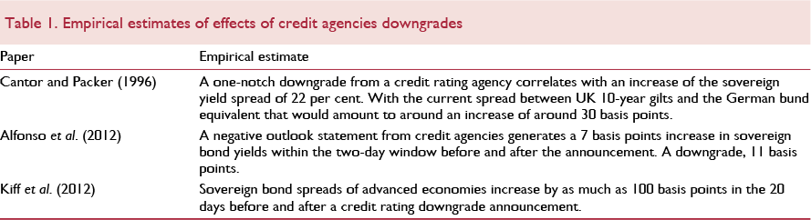
There is a question over the direction of causation between credit rating decisions and sovereign spreads. It could well be that agencies’ announcements are just a reflection of credit developments already factored in by the market and therefore carry no additional information. However, for the purpose of this analysis what is of relevance is not whether announcements trigger movements in spreads, but rather that announcements highlight times of heightened uncertainty on certain assets which allow calibrating movements in spreads derived from times of higher uncertainty.
Looking at the recent history provides some guidance as well. Figure 3 plots the spread of UK corporate AAA and BBB graded bonds over the 10 year gilt and figure 4 plots the credit default swap (CDS) spread on UK sovereign 5-year bonds. During the Great Recession, spreads of AAA graded corporates increased by 150 basis points and those of BBB graded bonds by around 600 basis points. The Eurozone sovereign debt crisis induced increases in spreads of 100 and 300 basis points for the AAA and BBB graded bonds, respectively. The UK CDS sovereign spread increased by at least 70 basis points during the great recession and by around 50 basis points during the Eurozone sovereign crisis. Note that data on CDS spreads already displays an increase of 20 basis points on the cost of insuring against default on UK sovereign debt over the past three months. Although we cannot map such an increase in the spread to a pricing in of the effects of a vote to leave it is hard to imagine that such an event bears no relation to the response of the cost of insuring.

Figure 3. UK corporate spreads to 10-year benchmark gilt (10-day rolling window)

Figure 4. UK credit default swap 5-year sovereign bond spread
Pooling all the information on the effects of credit rating agencies’ negative outlooks statements on bond spreads as well as the historical data gives us a range of conservative estimates falling between 30 to 100 basis points increase in the cost of financing following the period of heightened uncertainty that would start after a vote to leave. Our choice has been to err on the conservative side and we have implemented an increase of 50 basis points over a two-year window starting from the third quarter of 2016. We opt for the appeal of simplicity and shock the spread between loan and deposit rates that households face by 50 basis points as well. In practice this is akin to assuming that banks maintain their profit margins and pass the adjustment to their cost structure to households.
Equity premium
Not only should the cost of debt financing increase following the increase in uncertainty triggered by a vote to leave, but also the cost of equity. The fundamental factor that determines the cost of capital is unchanged: the expected stream of future dividends that companies can produce. However, this stream becomes much more difficult to forecast accurately given all the uncertainties that surround a vote to leave. From this perspective, we introduce a shock to the cost of equity finance equivalent to the shock we have introduced to debt finance: an increase in the spread over the risk free rate of 50 basis points that lasts for two years starting from the third quarter of 2016.
A brief look at the historical value of equity finance premium reassures us regarding the magnitude of the shock. Figure 5 plots the spread of the UK market wide dividend yield against the 10 year gilt yield; a measure of the equity premium. During the great recession the spread increased by around 300 basis points and during the sovereign crisis by around a 100 basis points. A rather surprising element observed in figure 5, that the spread kept increasing after the sovereign crisis, is explained by a continuous decline in the risk-free rate rather than an increase in the dividend yield of the UK stock market. From this perspective, the magnitude of our shock is well within the interval of possible increases in the spread following a period of heightened uncertainty.

Figure 5. UK equity premium
As a robustness check to our choice of the shock, we estimated an equation linking the spread on equity finance with our measure of uncertainty described previously.Footnote 7 We then obtained the increase in the spread that would result from a three standard deviation shock in our uncertainty measure that declines at an autoregressive rate of 0.5 per model period; a very similar shock to the one we have implemented in our main scenario. The outcome is very similar to the magnitude of the shock that we have implemented.
The outlook after a vote to leave the EU
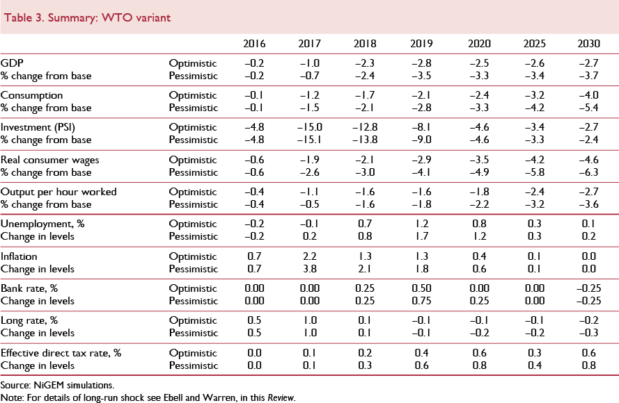
In our short-run scenario, we bring together each of the shocks discussed above. These are then layered in with the more structural long-run effects of the UK leaving the European Union that are discussed in the following paper in this Review by Ebell and Warren. The results of this simulation exercise are presented an an annual frequency in Table 3.
What we see is that on impact consumer price inflation jumps dramatically, figure 6. This is driven predominantly by the large depreciation of sterling, figure 7, which is itself a result of the widening of the risk premium. With the sterling effective exchange rate falling around 20 per cent on impact and remaining 14 per cent below the counterfactual in 2017, import prices rise and generate inflationary pressure in the consumption basket.

Figure 6. Inflation rate (percentage points difference from baseline)

Figure 7. Effective exchange rate (per cent difference from baseline)
Real GDP is broadly unaffected in 2016 as the decline in domestic demand is offset by a marginally positive net trade contribution, figure 8. This comes from a temporary terms of trade improvement as the depreciation of sterling boosts the price competitiveness of UK exporters, while reducing the attractiveness of imports to UK consumers. This is however short-lived and, by 2017, the domestic factors dominate, causing the level of GDP to fall to just over 1 per cent lower than in our baseline forecast.

Figure 8. GDP level (per cent difference from baseline)
Investment falls dramatically, figure 10. This comes through a number of channels. First is the direct impact of uncertainty. This shock in isolation results in a drop in business investment of just over 10 per cent in the third quarter of 2016, compared to the baseline case of a vote against leaving the EU, rising to 12½ per cent the following quarter before gradually returning to baseline levels. This direct effect is modest compared to other quantitative analyses. Reference Bloom, Floetotto, Jaimovich, Saporta Eksten and TerryBloom et al. (2014) for example simulate the effects of uncertainty on investment using a DSGE model calibrated using data on US firm's investment behaviour. They find that a 91 per cent increase in uncertainty results in a fall in investment of around 18 per cent. Similarly, Reference Bond and CumminsBond and Cummins (2004) investigate the effects of increasing uncertainty as measured by the standard deviation of daily stock returns on publicly traded US firms. They find that a 15 per cent increase in uncertainty reduces investment by 6 per cent.

Figure 9. Export and import volumes (per cent difference from baseline)

Figure 10. Private sector investment (per cent difference from baseline)
In addition to the direct uncertainty effect, we also observe a substitution effect between labour and capital as inputs which further weighs on investment. Falling real producer wages make labour a more cost effective input, while widening borrowing premia pushes up the user cost of capital, reducing the attractiveness of capital and lowering the optimal capital/output ratio.
Consumption is hit by lower real incomes alongside increased costs of credit and relative reductions in wealth as house prices fall, figure 11.

Figure 11. Household consumption (per cent difference from baseline)
Macroeconomic policy responses
The response of policymakers over this period will be extremely hard to predict. With this in mind, in our baseline counterfactual exercise we assume that the Monetary Policy Committee (MPC) chooses to wait for the uncertainty to subside before making a decisive policy move. As such, Bank rate is held fixed for the first two years of the simulation, until the third quarter of 2018. From this point on we assume the MPC reacts to the evolution of the economy by following a Taylor rule. This means that they set the short-term nominal interest rate in response to fluctuations in the output gap and deviations of inflation from its 2 per cent target rate. We parameterise this policy rule using the coefficients used in the Bank of England's own COMPASS model, as detailed in Reference Burgess, Fernandez-Corugeda, Groth, Harrison, Monti, Theodoridis and WaldronBurgess et al. (2013).
An interesting exercise is to see what effect our assumption of a fixed Bank Rate would have, compared to a world in which the MPC sets Bank Rate in line with its policy rule from the first instance. In this world, the policy rule as defined above would dictate that the Bank of England would loosen the stance of monetary policy by cutting Bank Rate by between 50 and 100 basis points relative to the counterfactual over the course of 2016 and 2017, figure 12. Based on the current market expectation of the path of Bank Rate, this would imply a move to zero, if not marginally negative, nominal interest rates.Footnote 8 To do this at a time when inflation is above target, as our scenario would suggest, may appear counterintuitive. However, as outlined previously, the bulk of the inflationary pressure stems from the sharp depreciation of sterling rather than a boom in domestic price pressures, which in fact would be likely to be softening. Therefore it may be that the MPC chooses to look through the temporary inflationary period in order to stimulate underlying demand and meet the mandated target more sustainably in the medium to long-term.

Figure 12. Bank Rate (percentage points difference from baseline)
We can see in figures 6–11 that allowing monetary policy to actively stabilise the economy from the off makes little difference to our central narrative. It does manage to reduce the spike in inflation in 2017 by around ½ percentage point, but with a trade-off in the shape of a marginally weaker outlook for GDP.
Within our simulation exercise, we make no allowance for unconventional monetary policies. If the MPC members feel they wish to stimulate the economy without implementing a negative policy rate, they have alternative policy instruments, most notably a fresh round of quantitative easing. By compressing the premia inherent in government bond yields, quantitative easing may be able to lower interest rates at the longer end of the yield curve and provide some additional stimulus.
The Bank of England also has responsibility for maintaining the stability of the UK's financial system. In this capacity senior Bank officials have already intimated that preparations have been made for large-scale liquidity provision in the event that a vote to leave creates unacceptable levels of market tension. If markets see the Bank as credible in this role of lender of last resort then the very promise to act may attenuate the worst of any market panic.
From the fiscal side, the budget position is worsened by 0.2 per cent of GDP in 2017 and 0.6 per cent of GDP in 2018, making it increasingly difficult for the government to achieve an absolute surplus by 2019–20, figure 13. Notably, the weaker performance of the economy may in fact provide increased fiscal space as within the current mandate there is a clause which states that the government no longer needs to achieve a budgetary surplus if GDP growth falls below 1 per cent per annum. The figures implied by our counterfactual exercise suggest that this would happen in 2018.

Figure 13. Government budget balance to GDP ratio (percentage points difference from baseline)
Transitioning to the longer run
None of the shocks detailed above persist beyond the 2-year negotiating period. This may seem a generous assumption, considering the potentially protracted nature of negotiations not only with the EU, but also with the rest of the UK's trading partners, both old and new. However, beyond this horizon we deem it likely that much of the uncertainty will have dissipated and markets will have a much clearer idea of the direction both the negotiations, and the UK economy, are taking, even if not all of the issues are fully resolved.
The counterpart to this waning uncertainty though is that as decisions are made and final positions taken, the more structural and permanent changes to the UK economy come into effect. As our uncertainty and premia shocks fade through 2017 and early 2018 there is a gradual introduction of changes to the UK's share of export markets, and eventually the imposition of tariffs. These second-phase shocks are detailed and discussed in Ebell and Warren, who analyse a range of post-EU arrangememnts for the UK. The results we have presented here have been derived on the assumptions within their WTO variant. For details of this, the readeer is referred to the work which follows. It must be noted that the ultimate long-run assumptions have consequences for our transition period. The forward-looking nature of agents means that, although subject to uncertainty, they do foresee, at least in part, the shifts that are ahead of them. The negative fallout from these later shocks in fact acts to weigh down on the performance of the UK even before they come in to effect.
Appendix A. National Institute Global Econometric Model (NiGEM): a non-technical overview
NiGEM is a global econometric model, and most countries in the EU, the OECD and major emerging markets are modelled individually. The rest of the world is modelled through regional blocks so that the model is global in scope. All country models contain the determinants of domestic demand, export and import volumes, prices, current accounts and gross foreign assets and liabilities. Output is tied down in the long run by factor inputs and technical progress interacting through production functions. Economies are linked through trade, competitiveness and financial markets and are fully simultaneous.
Agents are presumed to be forward-looking, at least in some markets, but nominal rigidities slow the process of adjustment to external shocks. The model has complete demand and supply sides; there is an extensive monetary and financial sector, together with household and government sectors. As far as possible the same theoretical structure has been adopted for each country. As a result, variations in the properties of each country model reflect genuine differences emerging from estimation, rather than different theoretical approaches.
Policy reactions are important in the determination of speeds of adjustment. Nominal short-term interest rates are set in relation to a forward looking feedback rule. Forward looking long-term interest rates are the forward convolution of future short-term interest rates with an exogenous term premium. An endogenous tax rule ensures that governments remain solvent in the long run; the deficit and debt stock return to sustainable levels after any shock, as is discussed in Reference Blanchard and FisherBlanchard and Fisher (1989). Exchange rates are forward looking and so can ‘jump’ in response to a shock.
Within NiGEM, labour markets in each country are described by a wage equation (see Reference Barrell and DuryBarrell and Dury, 2003 for a detailed description) and a labour demand equation (see, for example, Reference Barrell and PainBarrell and Pain, 1997). The wage equations depend on productivity and unemployment, and have a degree of rational expectations embedded in them – that is to say the wage bargain is assumed to depend partly on expected future inflation and partly on current inflation. The speed of the wage adjustment is estimated for each country. Wages adjust to bring labour demand in line with labour supply. Employment depends on real producer wages, output and trend productivity, again with speeds of adjustment of employment estimated and varying for each country.
We do not allow for an impaired interest rate channel or an increase in liquidity constrained consumers, while hysteresis effects in labour and capital markets are not a feature in NiGEM and so we do not address any of these effects that might materialise.


