


Introduction
Reference CookCook (1960) first proposed the glaciological use of impulse radars and by the late 1970s their value had become well established. For impulse sounding of glaciers, signals are commonly in the 1–20 MHz range, and data are observed optically or recorded photographically (Reference Sverrisson, Jóhannesson and BjörnssonSverisson and others, 1980; Reference Watts and WrightWatts and Wright, 1981) or as analogue signals on magnetic tape (Reference Jacobel and RaymondJacobel and Raymond, 1984; Reference Brown, Rasmussen and MeierBrown and others, 1986). The scientific potential of digitized data has been demonstrated (Reference Walford, Kennett and HolmlundWalford and others, 1986; Reference Jacobel and AndersonJacobel and Anderson, 1987) but most digital instruments in present use involve adaptations of laboratory equipment. Such equipment is cumbersome owing to requirements for environmental protection and suitable power sources. These factors led to our decision to develop a portable digital radar system. In this paper we describe the design and field testing of a prototype instrument.
Under ideal conditions, our system is capable of generating signals of approximately 4.5 kW instantaneous peak power, and detecting echoes to a depth of greater than 700 m. Range accuracy depends both on instrumentation and glaciological factors, but only the former are considered here. Our effective sampling rate yields an instrumentation precision of better than 1 m. The system is small, light (as little as 12 kg depending upon battery needs) and has low power consumption (11 W typical). Stability with respect to battery condition is ensured by using voltage regulators for all supply lines. A crystal-derived 1 MHz signal is included for field verification of time-base accuracy. With the exception of transmitter drift discussed below, no instabilities with respect to temperature were found. Echograms are collected and stored digitally under user or program control. The latter feature enables unattended operation so that temporal variations can easily be monitored. The system is organized as two separate units: a transmitter module and a receiver module (Figs 1 and 2). The transmitter unit consists of an antenna and a pulse generator which together generate an impulse having a band width of up to 20 MHz (the selection of the antenna determining the centre frequency). The receiver unit includes an identical antenna, a digitizing receiver, and a microcomputer of our own design. This microcomputer controls the acquisition of records and the operations of labelling, storing, retrieving, and displaying them. An optical cable links the two units, allowing the receiver unit to trigger the transmitter. Trace recording begins before the transmitter is triggered so that the complete surface wave is acquired and reliable timing is established.
A complete set of specifications appears in Table I. In the remainder of this paper we provide detailed descriptions of the transmitter and receiver units, discuss operational experience, and present representative data from our field seasons.

Fig. 1. Operating the U.B.C. impulse radar system from a back pack on Helm Glacier, British Columbia, Canada. Receiving unit and oscilloscope in the foreground are connected to the transmitter in the background by a fiber-optics cable.

Fig. 2. System block diagram.
Table I. Instrument Specifications

Note. All digital circuits use CMOS technology.
Transmitter
Pulse generator
Most impulse radar systems discussed in the literature (e.g. Reference Watts and EnglandWatts and England, 1976; Reference Sverrisson, Jóhannesson and BjörnssonSverisson and others, 1980) generate the required impulse of electromagnetic energy by delivering a single-phase voltage pulse to the terminals of an antenna designed to radiate over a broad band of frequencies. The voltage pulse is generated by using a solid-state switch to connect, as nearly instantaneously as possible, a charged capacitor directly to the antenna. Reference Watts and WrightWatts and Wright (1981) described a pulse generator of this type that uses for the high-speed switch a set of bipolar transistors operating in the avalanche mode. Such a design has many advantages. It is simple, inexpensive, has a voltage-rise time of a few nanoseconds, can develop a few kilowatts with a single transistor and can run either at a fixed rate as a relaxation oscillator or as a triggerable pulse generator. A conceptually similar system can be built using a silicon-controlled rectifier (SCR) as the switch (Reference Sverrisson, Jóhannesson and BjörnssonSverisson and others, 1980). Rise times are somewhat slower but SCRs are more efficient than avalanche transistors and reduce the total power requirements.
Our radar transmitter (Fig. 3) consists of two SCRs arranged back-to-back. Before switching, each one is holding off approximately 800 V at its anode. When they are simultaneously triggered by current pulses at their gates, the SCRs discharge a pair of capacitors into the antenna such that one arm of the dipole receives a 600 V positive pulse and the other arm receives a similar negative pulse. The resulting 1200 V pulse at the antenna terminals has an exponential rising edge which reaches a slew rate of 10.2 V/ns. As the anode voltages fall, the anode currents also fall until they drop below the so-called latching current. The SCRs then revert to their off conditions and the capacitors can recharge in time for the next trigger signal.
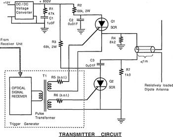
Fig. 3. Simplified circuit diagram of the transmitter referred to in the discussion of transmitter operation.
Common high-voltage SCRs (type 2N–6399) were used in the prototype transmitter. Although overall switching time is long, the avalanching process results in a fast slew rate. We have found that there is enough high-frequency energy contained in our switching wave form to drive 8 MHz (center frequency) antennas (see, for example, the results shown in Figure 4). It is the early part of switching that is slow and temperature-sensitive, and this is where costly SCRs such as the 2N–4204 could be expected to improve transmitter performance.

Fig. 4. Profile across a small unnamed glacier near Kaskawulsh Glacier in Yukon Territory, Canada, (a) Records were taken at 25 m intervals, using a transmitter and receiver spacing of 25 m. Antennas were oriented parallel to each other and parallel to the valley walls. Data were smoothed with a three-point moving average filter before plotting (equivalent to a low-pass filter with 34 MHz corner frequency). Note that some traces have echoes from both sides of the valley, and that echoes above the deepest points have been distorted by interference amongst closely spaced returns. Echo-range scale was calculated assuming V ice =168.2m/µs. (b) Ice-depth profile constructed by drawing arcs of echo range below each record. Echoes will have returned from surfaces tangent to these arcs.
Figure 3 is a schematic diagram of the power stage of the transmitter to which the following practical notes refer. (Complete specifications, circuit descriptions, and schematics can be found in Reference JonesJones (unpublished).) Capacitors C 2 and C 3 were chosen to be high-voltage ceramic disc capacitors of 0.01 µF, and R 2 and R 3 limit the charging rate to suit the small d.c.-to-d.c. converter used as a high-voltage supply (Venus Scientific, Inc. model C8T; converts 12Vd.c. at 190 mA to 800 V d.c). At the maximum charging rate, these capacitors take 4 ms to recharge, so the maximum pulse repetition rate is 250 Hz. Resistors R 4 and R 7 are required to reference the antenna to ground and to provide a slow discharge path for the charge delivered to the antenna arms. These resistors must be large enough to minimize reverse antenna currents, preventing a secondary radiated pulse.
The trigger generator converts the optical trigger signal into a current pulse suitable for forcing the SCRs into an avalanching condition. A pulse transformer, T1, with dual secondary windings ensures simultaneous timing of the two trigger currents, and resistors R 5 and R 6 are selected so that trigger currents are appropriate for the individual characteristics of each SCR. In this way, avalanche breakdown of both SCRs can be tuned to occur at precisely the same instant, as long as ambient conditions are identical, a condition ensured by placing the two devices adjacent to each other on the same heat sink.
During field trials we have found that overall timing is temperature-dependent, such that lower ambient temperatures result in greater delays between arrival of the trigger signal and emission of the radiated pulse. Delays of up to 3 µs were observed at temperatures as low as −15°C, the lower limit for reliable operation. This does not affect results because only the actual emission of the pulse is delayed. Since recording begins before the transmitter has fired, the time difference between receipt of the surface wave and receipt of the echo can be measured regardless of when the pulse is actually emitted. This is the chief advantage of synchronizing the transmitter to the receiver rather than the other way round.
The delay occurs because a greater charge (i.e. a longer current pulse) is required to initiate avalanching when semi-conductor junctions are at lower temperatures. This is not a fundamental problem. Use of higher-quality SCRs, temperature compensation, and more aggressive triggering would all contribute to more stable behaviour than that exhibited by our prototype.
This transmitter is not limited to use in triggered applications. For example, replacing the optical coupling section with a free-running oscillator would result in an efficient, self-contained impulse radar transmitter which could be used with a portable oscilloscope for a receiver in a manner similar to that described by Reference Jezek and ThompsonJezek and Thompson (1982).
Antennas
A broad-band antenna (one with good transient performance) is required to damp out natural resonances. A dipole antenna with this characteristic has been shown by Reference Wu and KingWu and King (1965) and by Reference Rose and VickersRose and Vickers (1974) to consist of dipole arms for which internal resistance increases towards the outer ends. The effect is to reduce the current as the pulse travels outward along the dipole arms, thus reducing reflections at the ends of the arms. The internal resistance profile that optimizes the impulse response (regardless of efficiency) can be found using relations derived by Reference Wu and KingWu and King (1965), with corrections by Reference Shen and KingShen and King (1965). They showed that a pure outward-travelling wave exists on an antenna arm of length h if the internal impedance, Z(x), at a position χ from the centre of the dipole, is given by

In Equation (1), the term Φ is the intrinsic impedance of the medium and Γ is the ratio of vector potential on the antenna surface to current along the antenna at the point where the current is a maximum. For this optimally damped antenna, Reference Shen and KingShen and King (1965) showed that the efficiency is around 9%. R 0 should be reduced to find a compromise between sufficient damping and adequate radiated energy for sounding. In general, R 0 would not be the same for different antenna lengths, nor would a single R 0 be optimum for a given antenna on different glaciers.
For our initial work, the approximate relationships given by Reference Wu and KingWu and King (1965) were evaluated in a manner similar to that of Reference Sverrisson, Jóhannesson and BjörnssonSverisson and others (1980) to yield R 0 ≈ 748.8 Ω A satisfactory compromise between efficiency and impulse response was attained using R 0 = 300 Ω, and the resistive loading was approximated by inserting fixed resistors of values found using Equation (1). These antennas have 5 m dipole arms that are built from 1 m lengths of 18 AWG copper wire with loading resistors at their midpoints. Each length is installed in a section of plastic pipe so that the antennas are rugged, collapsible, and can have loading resistors or length varied conveniently in the field. It should also be noted that, to minimize difficulties caused by transmission-line effects, the antenna should be connected directly to the current-pulse generator. Co-axial cable no longer than one-quarter of the minimum wavelength has been used successfully with our antennas.
The emitted frequency depends on the length of the antenna and the media in its vicinity. For a 5 m antenna half-length, our field results show that the energy radiated into the ice has a power spectrum peaking at 8.4 MHz, approximately consistent with that predicted for a simple dipole imbedded in ice (Reference JonesJones, unpublished).
The actual wavelet emitted when the antenna is excited by the input voltage step is difficult to estimate analytically because the current distribution on an antenna resting on an air/ice interface is not accurately known. However, the situation can be considered qualitatively. Our damped antenna is modelled as a resistor in series with a capacitor (Reference Wu and KingWu and King, 1965). A step voltage applied to the driving point will result in a “one-lobed” current pulse; that is, current will be in one direction and will first rise and then fall. The vector potential in the far field of an antenna is proportional to the first-time derivative of the current in the antenna. By the reciprocity theorem of antennas (e.g. Reference Jordan and BalmainJordan and Balmain, 1968, p. 345), the voltage on a receiving antenna is related in a similar way to the far-field vector potential, so the wave form recorded by the receiver will emulate the second-time derivative of the original current pulse. Therefore, if the pulse generator can impress a step voltage on to the antenna, the best possible zero-phase echo will be a three-lobed wave form.
Receiving Unit
A principal criterion for our radar receiver system was to obtain direct digital records. No commercial equipment could be found with the required degree of portability, so we designed and built the components ourselves. The present design includes a receiver amplifier, a sampling time-base (STB), an analogue-to-digital converter (ADC), a cassette tape for data storage, and a controlling computer.
The receiver amplifier is a general purpose, wide-band discrete transistor amplifier featuring fixed gain and variable front-end attenuation. The STB is a simplified version of one used in an airborne data-acquisition system described by Reference Narod and ClarkeNarod and Clarke (1983). For system control, we have developed a single-board microcomputer based on the GE/RCA COSMAC microprocessor series. Design criteria were low-temperature operation, compact packaging, a mechanically simple user interface, and flexibility in interfacing to peripherals. In all the components, many of the design choices were motivated by energy conservation. More detailed descriptions of the receiver-system components follow.
Receiver
The input stage of the receiver consists of a 0–40 dB variable attenuator which feeds the signal into a general purpose, five-transistor amplifier. The amplifier band width is at least 46 MHz, its voltage gain is 150, and its input impedance is 3600 Ω. This is very large when compared with an ideal matched load for an undamped dipole antenna (75 Ω) or, as for our design, about 300 Ω. However, many investigators have found that virtually any load functions well with a receiver antenna (e.g.Reference Watts and England Watts and England (1976) successfully used a 1 МΩ impedance oscilloscope as a receiver). We selected a value of 3600 Ω as a convenient input impedance for a high-speed, low-power transistor pre-amplifier.
Sampler
Our goal for depth resolution was 1 m. Using a velocity in ice of 170 m/µs yields a maximum sampling interval of 11.8 ns. We have achieved a 10 ns sample interval (100 MHz equivalent sample rate), without the high cost, large power requirements, and lower resolution of real-time digitizers, by using a sampling-time base similar to one described by Reference Narod and ClarkeNarod and Clarke (1983).
This sampling rate and our record size of 1024 points define a maximum observable two-way travel time of 10.24 µs. Because, in effect, we begin data acquisition before the transmitter is triggered, our recording interval is limited in practice to about 9 µs. Thus, our data-acquisition system is presently configured to observe a maximum depth of about 760 m.
Controller
As noted, our instrument is controlled by a microcomputer. This computer consists of a CDP1802 central processing unit, 4 kbytes of read-only memory (containing the program), 1.25 kbytes of random-access memory (used as a data buffer), and input/output ports for communication with peripheral hardware. These peripherals include: (i) a 16–key keypad with which the user enters commands and record identifiers, (ii) an eight-digit LED display to inform the user of the system status, (iii) a digital cassette tape recorder for permanent data storage, (iv) an RS–232C serial interface for transferring data to other devices, (v) digital-to-analogue converters for displaying a record on a small, low-power oscilloscope (the Tektronix model 211 has been used for all recent field work), and (vi) the sampling time-base receiver discussed previously. The entire system is under software control with the various functions initiated by the operator as instructions on the keypad. These can be classified as data collection, display, record identification, storage, and retrieval tasks, or as diagnostic functions.
Data are temporarily saved for viewing in the buffer memory, and then stored permanently on digital cassette tapes. Each record is saved as a separate file comprising 1024 eight-bit samples, and identification information entered by the operator. 25% redundant data storage, in the form of parity and cyclic redundancy characters, are included in the records and are available for error detection and correction. A maximum of 50 such records can be stored on standard digital data cassettes. The digital recorder/player and its control card are supplied by Memodyne Corporation (the model 333 “minicorder”).
Data are recovered by reading records from the cassette, either individually by file number or sequentially as a complete tape, and then released to another computing system through the serial interface. Processing that has been implemented so far includes: plotting, smoothing, signal differentiation, and time-dependent amplitude variation (Reference PragerPrager, unpublished), as well as trace shifting or truncation, alignment across a section, spectral analysis, principal-component decomposition of multi-trace sections, and amplitude processing (Reference JonesJones, unpublished).
Field Results
Twenty data sets, totalling roughly 1000 individual soundings, were collected in the 1986 and 1987 summer field seasons. On safe terrain, the entire procedure of moving to a new location, then collecting, inspecting, and storing a sounding record can be accomplished by an unassisted operator in 10 min. Field deployment and operating procedures that result in optimal system performance have been detailed in the literature (see, for example, Reference Watts and WrightWatts and Wright, 1981; Reference Jezek and ThompsonJezek and Thompson, 1982; Reference Cumming, Ferrari, Owen and MillerCumming and others, 1984; Reference Jacobel and RaymondJacobel and Raymond, 1984; Reference Walford, Kennett and HolmlundWalford and others, 1986). In agreement with most reports, our system performance is greatest when the two antennas are oriented along two parallel lines separated by approximately one wavelength. In addition, unambiguous results can be ensured only after considering certain local features of the field site. For example we have received echoes from nearby crevasses and buried morainal material. Also, wires on the glacier surface associated with independent experiments have been observed to ring sympathetically if they are placed parallel to and within roughly one-quarter wavelength of our antennas.
Figure 4 shows sounding results from a small unnamed temperate valley glacier near Kaskawulsh Glacier,Yukon Territory,Canada. The characteristic “bow-tie” pattern (Fig. 4a) is formed by the superposition of reflections from both walls of the subglacial channel. Records such as these are most likely to be obtained if antennas are placed parallel to the glacier margins. An arc-migrated ice-thickness interpretation (see Reference HarrisonHarrison, 1970) is given in Figure 4b.
On each trace in Figure 4a, a number of features can be recognized. After a short pre-trigger interval, the surface wave is prominent. Data were recorded using a high fixed gain, sufficient to cause severe clipping of the surface wave. Zero time was chosen as the rapidly falling edge of the surface wave. Because of phase inversion at the subglacial boundary, this feature corresponds to the rising edge of bottom reflections. For plotting, traces are aligned to the assumed zero reference and low-pass filtered to remove noise above 34 MHz; only the first 4 μs of each trace are shown.
Many other experiments have been performed on temperate and sub-polar glaciers. For example, we have studied signal propagation along the ice/air interface, echoes from crevasses, and glacier-bed reflection coefficients. Temporal variations of signal character over periods of 3–5 d were compared to other, independent but concurrent experiments, and an apparently mobile subglacial feature has been observed by comparing basal echoes from the same geographical location recorded in subsequent years. This work is currently in progress.
Conclusions
In general, we are pleased with the performance of this prototype instrument. Improving the medium for data storage is the highest priority. The digital cassette system currently in use draws a large proportion of the receiver power and is somewhat unreliable. Our favoured solution would be to replace it with solid-state memory. This would also speed up and simplify data transfer to a field computer.
Acknowledgements
This work has been supported by the Natural Sciences and Engineering Research Council of Canada and by Northern Scientific Training Grants from the Department of Indian and Northern Affairs. We should also like to thank Dr P. Johnson of the Department of Geography at the University of Ottawa, Ottawa, Canada, for supporting logistics of work around Kaskawulsh Glacier. Lastly, we thank the Superintendent and staff of Kluane National Park, Yukon Territory, Canada.


