


I. Introduction
Fine wine is increasingly viewed as a legitimate alternative asset for investors. In addition to funds targeting institutional investors, such as Sommelier Capital, new entrants with prominent backers are targeting the retail investor, such as Vinovest (minimum investment of $1,000) and Cult Wines ($10,000). Their timing may prove prescient. Historically, demand for alternative investments increases during periods of high uncertainty (Amenc, Martellini, and Ziemann, Reference Amenc, Martellini and Ziemann2009; Martin, Reference Martin2010), and recent evidence suggests fine wines provide diversification benefits to an equity portfolio (Maurer, Cardebat, and Jiao, Reference Maurer, Cardebat and Jiao2020). Yet, even as the market for fine-wine investment matures, basic questions about portfolio management remain unanswered.
Asset selection is fundamental to portfolio management. While the set of investment-grade fine wines continues to expand (e.g., Masset, Weisskopf, and Fauchery, Reference Masset, Weisskopf and Fauchery2020), the majority of the literature on the returns to investing in fine wines focuses on the five first-growths of Bordeaux's Left Bank (c.f., Le Fur and Outreville, Reference Le Fur and Outreville2019). In this paper, I address the asset selection question: over the long run, has it been better to invest in wines from the superstar châteaux of the Left Bank, Right Bank, or both? Specifically, I analyze the long-run returns to investing in the five first-growths of Bordeaux's Left Bank, plus three superstar châteaux from its Right Bank: Ausone, Cheval Blanc, and Petrus.
There are a variety of reasons why the Right Bank might be an attractive investment. As I show using expert reviews from Global Wine Score (Cardebat and Paroissien, Reference Cardebat and Paroissien2015), quality is virtually indistinguishable across the two Banks. On the Right Bank, supply is far more constrained. For example, the vineyard area of Ausone is a fraction (1/15th) of that of Lafite (Anson, Reference Anson2020). Further, vintage variation may not be perfectly correlated because of differences in varietals, soil, microclimate, and other production conditions (Bois et al., Reference Bois, Joly, Quénol, Pieri, Gaudillère, Guyon, Saur and Van Leeuwen2018). Thus, adding wines from the Right Bank to a portfolio of wines from the Left Bank could provide diversification benefits. However, demand for the Right Bank has experienced less fantastic growth, perhaps because its exclusion from the 1855 Classification allowed it to escape the attention of newer oenophiles.
To analyze returns, I hand-collected prices for the period 1938–2017 from an archive of retail catalogs from Sherry-Lehmann Wine & Spirits Merchants, a retailer in New York City. I supplement this data with prices from the London International Vinter's Exchange (Liv-Ex), which is based on transactional information from around the world. My data is like that of Dimson, Rousseau, and Spaenjers (Reference Dimson, Rousseau and Spaenjers2015), which studied the five first-growths of Bordeaux over 1900–2012 using hand-collected prices from a historical archive of auction catalogs provided by Christie's London, supplemented with records from London-based retailer, Berry Bros. & Rudd. Even though my sample is shorter—because it is from the United States, it necessarily begins at the end of Prohibition—it offers the advantage of being 11.0% larger (35% larger counting Right Bank wines). After merging the data from my two sources, I analyze the long-run returns to investing in eight superstar châteaux from Bordeaux using two complementary approaches, again following Dimson, Rousseau, and Spaenjers (Reference Dimson, Rousseau and Spaenjers2015).
First, I examine how the price of wine evolves as it ages. I find that the prices of the five first-growths increase monotonically over time. The path of their prices is nonlinear, increasing at an increasing rate over time: at age-50, the wine is about seven times more expensive than an age-0 wine; at age-100, it is about 30 times more expensive than an age-0 wine. My pattern of monotonically increasing prices in wines from the Left Bank is virtually identical to the pattern found in Dimson, Rousseau, and Spaenjers (Reference Dimson, Rousseau and Spaenjers2015).
Interestingly, wines from the Right Bank follow a very different path: prices increase at an increasing rate until age-50, peak at age-60, and then decay toward 0 as they approach age-100. Prices for Right Bank wines also start at a higher base, with an age-0 wine twice as expensive. They stay more expensive until age-70. Their prices peak around age-60, when they are about 15 times more expensive than an age-0 wine from the Left Bank. From an investor's perspective, this different life cycle in prices could provide diversification benefits. This is because, with respect to the returns to aging, the path of prices across the two banks is uncorrelated.
Second, I evaluate the performance of investing in the superstar châteaux of Bordeaux over the 80 years of my sample. Of course, as highlighted in the review of Le Fur and Outreville (Reference Le Fur and Outreville2019) and further considered in Masset et al. (Reference Masset, Weisskopf, Cardebat, Faye and Le Fur2021), I am not the first to consider the long-run returns to investing in fine wine. Le Fur and Outreville (Reference Le Fur and Outreville2019) review 46 papers published from 1978 to 2018 on the rate of return from investing in fine wines. Most focus exclusively on the five first-growths from the Left Bank. Those that do include the superstar châteaux of the Right Bank have limited sample periods, with most using 10–15 years of price data or less; for example, 1983–1998 (Ali and Nauges, Reference Ali and Nauges2007), 2001–2010 (Chu, Reference Chu2014), and 2007–2013 (Bocart and Hafner, Reference Bocart and Hafner2015). Thus, my results are unique in their long-run focus on returns from investing in Bordeaux, inclusive of the Right Bank.
Using the repeat-sales method of Shiller (Reference Shiller1991), I find the geometric-average rate of return was 6.78% in real terms for the period 1938–2017. The difference between the joint portfolio and only wines from the Left Bank is less than 0.01%. I find the joint portfolio has a higher ex post Sharpe-ratio than a portfolio of wines only from the Left Bank when the risk-free rate is less than 6.95%. Thus, over the long run, adding Right Bank wines to the portfolio does provide a diversification benefit. Note that my 6.78% return for the period 1938–2017 is higher than the 5.3% in Dimson, Rousseau, and Spaenjers (Reference Dimson, Rousseau and Spaenjers2015) for 1900–2012. This is because less of my sample is from before 1960, after which Dimson, Rousseau, and Spaenjers find that returns accelerated.
The remainder of this paper proceeds as follows. In Section II, I describe the data, including the collection process for historical prices from the archive of Sherry-Lehmann catalogs. In Section III, I use hedonic regression to examine the life cycle of prices with respect to aging. In Section IV, I use repeat sales price indexes to evaluate the appreciation of prices in real terms over the long run. Section V concludes.
II. Data
A. Wine selection
The Gironde estuary bifurcates Bordeaux into two major subregions: the Left and Right Banks. I focus on eight red wines from the superstar châteaux of Bordeaux: the five “first growths” of the Left Bank (Haut-Brion, Lafite Rothschild, Latour, Margaux, and Mouton Rothschild), and three superstar châteaux on the Right Bank: Ausone, Cheval Blanc, and Petrus. I exclude at least two worthy candidates for superstar châteaux on the Right Bank: Le Pin and Lefleur. I exclude the former because it was founded in 1979 and, unlike the other wines, was not widely distributed. I exclude the latter because Sherry-Lehmann did not promote it as a first growth or equivalent (i.e., on par with Lafite, Latour, etc.) in their catalogs.
All are undoubtedly among the world's most prestigious and expensive wines. Current average retail prices range from $775 (Haut-Brion) to $4,760 (Petrus).Footnote 1 All personify the Bordeaux style: rich, full-bodied, and tannic wines, which are aged for extended periods prior to release in new oak barrels and have long aging potential.
The wines have broadly similar attributes. Start with expert scores, a tangible if imperfect proxy for quality, with well-known impacts on prices. Let S ivt be the average, standardized score for château-vintage (i, v) at time t. I estimate the regression:
where a i and b v are fixed effects for château and vintage, respectively. I use robust standard errors, clustered by year of review. I use scores standardized by expert from Global Wine Score (Cardebat and Paroissien, Reference Cardebat and Paroissien2015).Footnote 2 I estimate Equation (1) using data from January 1996 to December 2018. For brevity, I evaluate expert scores using the 95% confidence intervals for $\widehat{{a_i}}$ , which represents the average score for a given château across critics, holding vintage constant.
The expert scores are practically identical. The lowest-scoring wines were Cheval Blanc (93.8, 95.0) and Mouton (94.0, 95.0). The median-scoring wines were Ausone (94.7, 95.7) and Lafite (94.8, 95.7). The highest-scoring wines were Latour (95.1, 96.1) and Petrus (94.9, 96.1). These scores illustrate that wine quality—relative to the universe of reviewed wines, not just relative quality within Bordeaux—is high and statistically indistinguishable. Outside of scores, it is interesting to note that all were established prior to c1837. All, except Petrus (located in a commune without an official classification), hold the highest designation in their respective communes.Footnote 3
While broadly similar, there are notable differences across the wines (Parker, Reference Parker2005; Anson, Reference Anson2020). The wines from the Left Bank are dominated by Cabernet Sauvignon grown on gravel soils, with the balance being a blend of Merlot, Cabernet Franc, and Petit Verdot. Cabernet sauvignon comprises approximately 45% of Haut-Brion, 70% of Lafite, 75% of Latour and Margaux, and 77% of Mouton. Ausone, Cheval Blanc, and Petrus do not use Cabernet Sauvignon. The wines from the Right Bank are dominated by Merlot and Cabernet Franc—50%–50%, 42%–58%, and 95%–5% for Ausone, Cheval Blanc, and Petrus, respectively—on clay or limestone. As a result, wines from the Right Bank are characteristically softer and more approachable. A second notable difference is production, which is much lower on the Right Bank. Cheval Blanc is the largest producer on the Right Bank at roughly 96,000 bottles/year, and Ausone is the smallest at less than 24,000. On the Left Bank, the largest is Lafite at 300,000 and the smallest is Haut-Brion at roughly 132,000. Vineyards on the Right Bank are smaller (7–39 versus 53–100 ha), older (35–50 versus 30–50 years), and less productive (35–36 versus 40–51 hL/ha). These attributes provide further credence to the argument that wines from the Right Bank might provide some diversification benefits to a portfolio of Left Bank wines.
B. Sherry-Lehmann catalogs
On March 6, 1934, the well-known bootlegger and whiskey connoisseur Jack Aaron founded Sherry Wine and Spirits Co., Inc. in the Louis Sherry building on Madison Avenue in New York City. Jack's brother, Sam, joined in 1935 and led the wine side of the business. In the 1940s, Sam befriended another wine and food lover, James Beard, who often contributed to the company's catalogs. In 1965, Sherry acquired its largest competitor, M. Lehmann, a gourmet grocer, and became Sherry-Lehmann Wine & Spirits Merchants. Today, Sherry-Lehmann operates a three-floor, 9,000-square-foot retail location on Park Avenue as well as a 65,000-square-foot climate-controlled storage facility.
Shortly after the repeal in 1935, Sherry-Lehmann issued its first catalog, where my sample begins. I collected list prices from all the Sherry-Lehmann catalogs archived in the UC Davis Library Digital Collections.Footnote 4 I recorded the prices of the eight wines for any reported vintage and annotated offers with nonstandard bottle sizes or future delivery. In total, I collected 10,885 prices from 391 catalogs for the period 1935–2010.
Two substantive complications arose during data collection. First, several catalogs were undated, ambiguously dated, or incorrectly dated. I re-labeled their dates through context clues such as the youngest vintage of an available white wine and the vintages of futures on offer. For example, the summer catalog for year T would have white wines as young as year T − 1 and futures from year T − 1 and T − 2, not T or T − 3.Footnote 5 Second, quotes become scarce toward the end of the sample (when the wines of interest become quite expensive). I supplement the catalogs with data on prices provided by the London International Vintners Exchange (Liv-Ex) from June 2005 to January 2017. Liv-Ex collects daily transaction records on the price of fine wines exchanged through global secondary markets. Price updates are collected through over 400 member distributors and auction houses around the world, accounting for approximately 35,000 transactions worth $30 million daily. These indices, which aim to reflect current and past market conditions, are reported by professional data vendor services including Bloomberg and Thomson Reuters. I convert Liv-Ex prices to U.S. dollars using exchange rates from Officer (Reference Officer2021) and average monthly prices on a quarterly basis.
Other complications were easily remedied. Several catalogs are duplicated in the archive. After data collection was complete, I cross-checked my records and removed duplicated catalogs. The archive includes other documents mailed to customers, such as special offers. I include these in the records if pertinent. Typically, prices were listed on both a per-bottle and per-case basis. However, sometimes they are listed in only one of the two denominations. I recorded prices on a per-case basis. When listed only on a per-bottle basis, I assume bottles cannot be purchased at a quantity discount and multiplied by 12, which I would argue is reasonable because these listings tend to occur when the wine is very old, rare, and expensive. For nonstandard bottles, I converted the quantity to the size of a standard 9 L case, annotated the entry with the bottle size, and adjusted the price if necessary (i.e., multiply the quoted price for a 6.0 L Methuselah by 1.5).
C. Summary statistics
Table 1 reports summary statistics for my final database of prices. In total, I collected 10,885 records from the Sherry-Lehmann catalogs for the period 1938–2017. The Liv-Ex data, which is a rolling portfolio of the ten most recently released vintages, added 481 observations for each of the eight wines for 2005–2017. Each observation is a wine-vintage pair (e.g., Haut Brion 2010) dated on a quarterly basis (e.g., 2015Q2), with additional information on the transaction type (e.g., Liv-Ex or catalog), bottle size (all Liv-Ex records are for standard bottles), and futures (all Liv-Ex records are for released wines). There are 1,428 unique wine-vintage combinations included in the database. I deflate nominal prices to a base of 2015Q1 using the U.S. CPI (U.S. Bureau of Labor Statistics, 2021).
Table 1. Summary statistics
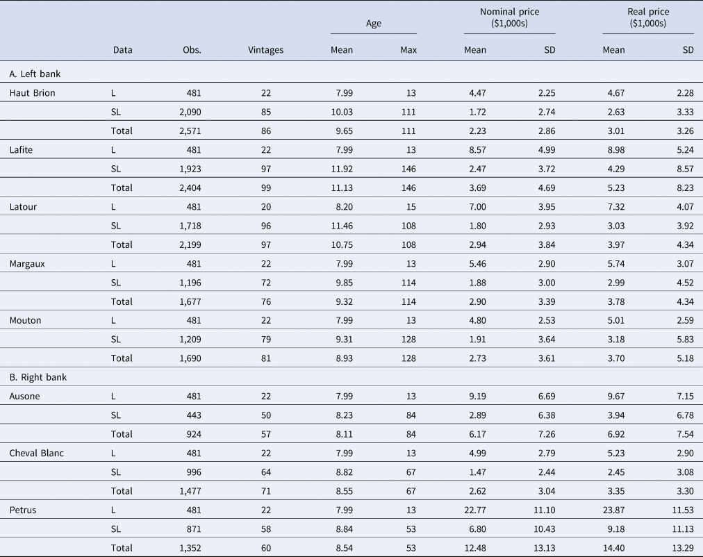
Note: L - world market data from Liv-Ex; SL - retail data from Sherry-Lehmann catalogs; Total - two data sets merged together.
Panel A of Table 1 reports summary statistics for wines from the Left Bank and Panel B for wines from the Right Bank. Reflective of their relative scarcity, there are 924–1,352 observations for wines from the Right Bank compared to 1,677–2,571 from the Left. They also tend to be younger: average ages of 8.11–8.55 versus 8.93–11.13 and maximum ages of 53–84 versus 108–146. On average, real prices range from $3,102/case ($259/bottle) for Haut Brion to $14,403 ($1,200/bottle) for Petrus.
III. Aging and prices
In this section, I examine the relationship between wine prices and aging. To do so, I estimate a hedonic regression of wine prices by age, controlling for factors such as sale location, châteaux, bottle size, year of sale, quarter of sale, and future offer. I also show how the number of listings per year changes by wine age.
A. Estimation
I begin my analysis of the long-run returns from investing in Bordeaux by examining how aging affects prices. Let P ivℓt be the price of wine from château i and vintage v at location ℓ in period t. I estimate the hedonic regression:

where α i is a château-level fixed-effect, D i is an indicator equal to 1 if wine i is from the Right Bank and 0 otherwise, $x_{iv\ell t} = [ {Age, \;Age^2, \;Age^3} ]$ is a cubic in age, and z ivℓt is a vector of controls. Controls include a series of fixed effects for location, bottle size, year of sale, quarter of sale, and future offer. The interaction between the cubic in age and indicator for wines from the Right Bank allows examination of the differences in the age cycle across wines from the Left and Right Banks. One caveat to this approach identified by Breeden (Reference Breeden2022) is that, if low-quality vintages tend to disappear from the data due to nonrandom selection, price effects for older wines may contain a degree of upwards bias.
B. Results
Table 2 reports least-squares estimates of Equation (2) with robust standard errors clustered by year of sale. Before examining the relationship between age and price, I examine the effects of other variables on prices. Quoted prices from Liv-Ex, which reflect world prices, are systematically lower than local and landed prices at Sherry-Lehmann. Turning to château-level fixed-effects, where Ausone is the omitted category, we see only Petrus and Lafite tend to be more expensive than Ausone, regardless of vintage, time, or age. Wines from all the other châteaux tend to be less expensive, with Haut Brion being the least expensive, followed closely by Cheval Blanc. Price and production quantity are clearly not perfectly correlated: Lafite is the biggest, while Haut Brion and Cheval Blanc are among the smallest. Other effects, which are omitted from the table for brevity of presentation, are consistent with expectations: nonstandard bottle sizes trade at a significant premium; prices are significantly higher during the fourth quarter; and wines sold as futures trade at a small discount (e.g., Oleksy, Czupryna, and Jakubczyk, Reference Oleksy, Czupryna and Jakubczyk2021).
Table 2. Results of hedonic regressions
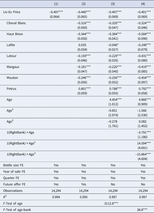
Note: *p < 0.10; **p < 0.05; ***p < 0.01.
Figure 1 illustrates the estimated relationship between aging and prices. The top panel plots the effect of aging on price using the full model from Column (4) of Table 2, with the Left Bank illustrated with a solid line, the Right Bank with a dashed line. The results for the Left Bank are broadly consistent with Figure 4 in Dimson, Rousseau, and Spaenjers (Reference Dimson, Rousseau and Spaenjers2015). Most importantly, prices increase monotonically in age for wines on the Left Bank. The shape of my relative price line better traces the curvature of Dimson, Rousseau, and Spaenjers (Reference Dimson, Rousseau and Spaenjers2015)'s line for low-quality vintages (i.e., it is not concave between age 0–50), reflecting that my estimates are a weighted average of their low- and high-quality vintages. While the slope of my relative price line appears steeper (e.g., crosses 10 between ages 50–60 rather than 70–80), it may not be different because the base value (which is used to set the intercept to unity) of the intercepts across the two graphs is different.

Figure 1. Price and quantity by age.
The shape of the Right Bank's line is the most interesting feature of the top panel of Figure 1. In contrast to the Left Bank's monotonically increasing prices, the Right Bank's line is concave. At age 0, Right Bank wines are more than twice as expensive. Even from that higher base, the Right Bank's line increases at a much faster rate: the Right Bank crosses 10 at age 40, compared to the Left Bank at age 59. The Right Bank peaks at a value of 15.4 at age 60. At age 60, the value of a Left Bank wine is only 10.4. The two lines intersect at age 68. While the Left Bank continues to increase in value, reaching 28.8 at age 100, the Right Bank rapidly deteriorates. By age 76, the Right Bank is below 10, by age 85 it is below 5, and at age 97 it falls below 1—after 97 years, it is worth less than an aged 0 wine from the Left Bank. In other words, wines from the Right Bank reach peak maturity around age 60, but—unlike their Left Bank counterparts—beyond maturity do not continue to increase in value. As an asset, they have a different life cycle, which has implications for their optimal mix in a portfolio.
The bottom panel of Figure 1 illustrates the quantity of wines available by age. Specifically, it reports the average number of listings per year in the Sherry-Lehmann catalogs by age. In the catalogs, most listings are for wines between ages 5–8, followed closely by ages 1–4. Beyond ages 5–8, the number of listings decreases as the wines age. The share of Right to Left Bank wines is also highest between ages 1–4 (31.3%) and 5–8 (31.6%), before it decreases over time from between 17.6–23.3% over ages 13–28 to between 9.7–14.0% over ages 29–40 and 13.9% for over the age of 40. Perhaps not surprisingly, wines at auction tend to be slightly older (peaking at ages 10–13), but otherwise follow a similar pattern (Dimson, Rousseau, and Spaenjers, Reference Dimson, Rousseau and Spaenjers2015, Fig. 5.).

Figure 2. Long-run returns to investing in Bordeaux.
IV. Long-run returns
In this section, I examine the return on investment for the superstar châteaux of Bordeaux's Left and Right Banks from 1938–2017. The primary goal of my analysis is to evaluate the risk and return benefits of adding Right Bank wines to a portfolio of Left Bank wines.
A. Estimation
I evaluate the long-run returns of investing in Bordeaux wines using a repeat-sales estimator (Bailey, Muth, and Nourse, Reference Bailey, Muth and Nourse1963; Shiller, Reference Shiller1991). This estimator uses the subset of wine-vintage pairs (e.g., Haut Brion 2000), which appear at least twice in the final database of prices. Aggregating sales across quarters within a year, I have 521 unique wine-vintage pairs that appear at least twice. All but 60 of these unique wine-vintage pairs appear more than three times. I encode these multiple sales as separate, consecutive pairs of repeat sales (Shiller, Reference Shiller1991, p. 122). After doing so, there are J =3,714 repeat sales with price P jt in period t for j = 1, …, J.
The reciprocal price index to be estimated is π t. Without loss of generality, assign the base period 0, such that t = 0, 1, …, T, and assign 1 to the value of the index in period 0, π 0 = 1. Then π is a T-length vector of coefficients. I use the interval- and value-weighted arithmetic repeat sales (IVW-ARS) estimator of Shiller (Reference Shiller1991), which is estimated with feasible generalized least-squares:
The dependent variable of the jth repeat-sale, Y j, is the value of the repeat sale in the base period, P j0, and 0 otherwise. The independent variable, X, is a J × T-matrix with element X jt equal to −P jt if t is the first entry of the repeat sale, +P jt if t is the second entry of the repeat sale, and 0 otherwise. Analogously, the instrumental variable, Z, is a J × T-matrix with element Z jt equal to −1 when the first repeat sale was in time t, +1 when the second repeat sale was in time t, and 0 otherwise. To account for the correlation across rows introduced by the encoding of multiple sales, the J × T variance matrix, Ω, is block diagonal, with blocks corresponding to individual wine-vintage pairs and each block tridiagonal. In the application of Equation (3), Ω is replaced with its estimate from a first stage assuming Ω = σ 2I.
B. Results
The top panel of Figure 2 plots the price index in real USD, $\widehat{{\pi ^{{-}1}}}$ , estimated using the IVW-ARS method. The index is set to one in the base year, 1938. I linearly interpolate the index for 1939–1945 and 1982–1985, periods for which there are no catalogs in the archive. The price index can be interpreted as the return to the portfolio of holding one of each wine-vintage pair from 1938 to 2017.
First, consider the index for wines exclusively from the Left Bank (black). Real prices grew steadily from 1940–1960: from 1 in 1938, to 1.4 in 1950, to 2.15 in 1960. Then prices began to accelerate, reaching 7.0 in 1970 before growing by a factor of more than four to reach 30.8 in 1980. Growth leveled from 1980 to 1995. Then, growth rapidly accelerated again: from 1995 to 2000, prices jumped from 39.9 to 120.9. Prices again more than doubled in the next decade, reaching 260.9 in 2010. Prices peaked at 311.9 in 2011, but have since receded, ending at 190.2 in 2017. Over the full sample of 80 years from 1938 to 2017, the geometric average annual real return was 6.78%. This is slightly higher than Dimson, Rousseau, and Spaenjers’ (Reference Dimson, Rousseau and Spaenjers2015) estimate for the period 1900–2012, which is not surprising given that they find prices were relatively flat between 1900–1940, and broadly consistent with others (c.f., Le Fur and Outreville, Reference Le Fur and Outreville2019).
Second, consider the index for wines from both the Left and Right Banks, illustrated in gray. This joint index follows the Left Bank index closely, with a correlation of 0.998. Although the joint index ends slightly higher (190.6), the joint index is lower than the Left Bank index in all but four periods, and the median difference between the two indices is –5.81%. Overall, the joint index appears to have slightly lower returns. The question is whether this lower return is offset by lower risk. In other words, whether there is a diversification benefit to investing in both Banks.
The bottom panel of Figure 2 plots nominal returns on an annual basis, that is:

the percentage return from buying and selling the portfolio each year. The (arithmetic) average nominal return on the Left Bank index is 9.95%, compared to 9.81% for the joint index. That is, in an “average” year, both portfolios earned a nearly 10% return. While the return on the joint index is lower, so too is the standard deviation of returns: 0.193 versus 0.201. Thus, the coefficient of variation is slightly smaller for the joint index: 1.96 versus 2.02.
Investors summarize the risk-return trade-off using the Sharpe (Reference Sharpe1964) ratio:

where R p is the return of the portfolio, R f is the return of a risk-free asset, and σ p is the standard deviation of the excess return to the portfolio. A higher Sharpe ratio means a greater return relative to the level of risk. Consider ex post Sharpe-ratios for the two portfolios, which are calculated using the nominal annual returns. At a risk-free rate of 1.0%, the Sharpe ratio increases from 44.4 to 45.8 by adding Right Bank wines to the portfolio. At 0%, it increases from 49.4 to 51.0. At 5.0%, from 24.6 to 25.0. In fact, if the risk-free rate is less than 6.95%, the joint index has a higher Sharpe ratio than the index with wines exclusively from the Left Bank. The long-run risk-free rate is typically considered between 3–4%. Thus, over the long run, the diversification benefit from adding Right Bank wines has been worth the slightly lower returns.
V. Conclusion
Fine wine has increasingly received attention from investors seeking to bolster their portfolios with alternative assets. Investors are attracted to its relatively high real returns and low correlation to equity markets. Most studies of returns from fine wine focus on the five “first growth” wines of Bordeaux, all located on the Left Bank. I consider superstar wines from Bordeaux's Right Bank, which are equally appreciated by experts but less well-known among fine-wine consumers at-large. I have two main findings. First, the prices of wines from the Right Bank follow a very different life cycle with respect to age than their counterparts from the Left Bank. Whereas Left Bank prices ascend monotonically, Right Bank prices start at a higher base, accelerate faster, and peak at age-60, before deteriorating. Second, a portfolio of Left and Right Bank wines outperformed a portfolio of exclusively Left Bank wines after adjusting returns for risk. Future work might consider incorporating vintage quality using weather data and examine the implications of the different life cycles for the optimal portfolio. It might also consider the forward-looking opportunities for wines from the Right Bank as the number of consumers grows, the knowledge among consumers grows, and the limited size of wineries on the Right Bank becomes an increasingly binding constraint on supply.
Acknowledgments
I thank Karl Storchmann and an anonymous reviewer for reviewing the paper. I thank Julian Alston for helpful comments and presenting the paper at AAWE 2022. I thank Sherry-Lehmann, Roy Brady, and Arnold A. Bayard for their contributions of the catalogs to UC Davis Library's Archives and Special Collections, as well as Liv-Ex and Global Wine Score for data access. Competing interests: The author declares none.


 Open access