


1. Introduction
Hypersonic vehicles are usually accompanied by shock–shock interactions and shock wave/boundary layer interactions (SWBLIs), which may cause extremely high heat flux peaks on the surface (Wieting & Holden Reference Wieting and Holden1989) or unsteady oscillation of the flow field (Zhong Reference Zhong1994). Edney (Reference Edney1968) first summarized the shock interactions into six types according to the relative position of the oblique shock and bow shock. Furthermore, Hains & Keyes (Reference Hains and Keyes1972), based on oblique shock and Prandtl–Meyer expansion wave theory, developed theoretical and empirical formulations for the prediction of pressure/heating peaks. In particular, the correlation between pressure and heat flux peak is of great practical value for engineering (Grasso et al. Reference Grasso, Purpura, Chanetz and Délery2003). However, these correlations are based on some typical configurations, such as the supersonic compression ramp or the oblique shock impinging on a flat plate. The applicability of the correlation to complex shock interactions needs further development (Li et al. Reference Li, Zhang, Wang and Yang2019).
With the development of hypersonic airbreathing vehicles (see figure 1a), a V-shaped blunt leading edge (VSBLE) (see figure 1b) of the inlet has been noted by researchers (Malo-Molina et al. Reference Malo-Molina, Gaitonde, Ebrahimi and Ruffin2010). Xiao et al. (Reference Xiao, Li, Zhang, Zhu and Yang2018) first extracted the VSBLE configuration from vehicles and defined the main geometric parameters including the half-span angle β, the leading-edge radius r and the crotch radius R. Based on this model, Li et al. (Reference Li, Zhang, Wang and Yang2019) and Wang et al. (Reference Wang, Li, Zhang, Liu, Yang and Lu2018) studied the pressure–heat flux correlation and unsteady shock oscillation around the VSBLE. Furthermore, Zhang et al. (Reference Zhang, Li, Huang and Yang2019a, Reference Zhang, Li and Yang2021a) combined experiments, numerical simulations and theoretical analysis to explore the shock structures around the VSBLE with a wide range of geometric parameters. Among them, the VSBLE with R/r = 3.25 and β = 24° has attracted much attention. The self-induced shock interactions cause extremely high heat flux peaks that can be up to seven times the stagnation-point value, which is computed from the Fay–Riddell (F-R) theory (Fay & Riddell Reference Fay and Riddell1958). However, the free stream adopted in the above studies is Mach 6. Note that the working condition of airbreathing hypersonic vehicles with hydrogen fuel scramjet engines can be up to Mach 12 or higher (Reubush, Nguyen & Rausch Reference Reubush, Nguyen and Rausch2004). Studies (Wieting & Holden Reference Wieting and Holden1989; Boldyrev et al. Reference Boldyrev, Borovoy, Chinilov, Gusev, Krutiy, Struminskaya, Yakovleva, Délery and Chanetz2001) show that as the Mach number increases, the detached shock moves closer to the wall and the heating load has an increasing trend. Therefore, it is crucial to explore the flow characteristics of VSBLE at a higher Mach number.

Figure 1. (a) Mach contour of a hypersonic airbreathing vehicle with a VSBLE (in the red frame). (b) Volume streamlines (coloured by the Mach number) and heat flux of the VSBLE.
However, the purpose of exploring the flow mechanism and predicting heat flux peaks is for better control and protection in aircraft design (Liu et al. Reference Liu, Kang, Yan, Sun and Jiang2022; Zhou et al. Reference Zhou, Liu, Lu, Kang and Yan2022). In particular, shock control methods can effectively reduce the adverse effect caused by SWBLI (Ashill, Fulker & Hackett Reference Ashill, Fulker and Hackett2005). Among many shock control devices, the shock control bump (SCB) is a passive control device with a simple shape, high robustness and low profile drag (Bruce & Colliss Reference Bruce and Colliss2015).
As the name suggests, an SCB is a physical bump mounted on an aerodynamic surface. It was first applied to the upper surface of transonic wings (Birkemeyer, Rosemann & Stanewsky Reference Birkemeyer, Rosemann and Stanewsky2000), as shown in figure 2(a). The so-called smearing effect of the SCB can split the near-normal shock into a weaker λ shock structure of the wing surface, which can reduce the total pressure loss and drag (Qin, Wong & Le Moigne Reference Qin, Wong and Le Moigne2008). Recently, researchers explored the application of the SCB in supersonic flow with an incident shock (see figure 2b). Based on the cowl shock/boundary layer interaction in a supersonic inlet, Zhang et al. (Reference Zhang, Tan, Li and Yin2019b) investigated the control effect of a shape-memory alloy bump by experimental and numerical methods. The shock-induced large separation bubble transformed into two small-scale separation bubbles under the control of the deformable bump. Schülein, Schnepf & Weiss (Reference Schülein, Schnepf and Weiss2022) proposed a new SCB contour shape called the concave bump, which is marked by an expansion kink directly at the peak. The highest values of separation-length reduction were up to 100 %.

Figure 2. Principle of SCB operation: (a) on a supercritical wing with a near-normal shock and (b) on a supersonic flat plate with an incident shock.
However, the application of an SCB in the hypersonic flow has hardly been explored. It should be noted that the SWBLI-induced extremely high heating loads become a primary problem under hypersonic conditions (Wieting & Holden Reference Wieting and Holden1989). The smearing effect of the SCB gives us the idea that the SCB can be used not only to suppress separation but also to eliminate the pressure/heating peak near the shock impingement. Therefore, this paper extends the application of an SCB to hypersonic flow as a thermal protection strategy.
Moreover, as with all flow control devices, the SCB may be ineffective or have adverse effects under off-design conditions. Bruce & Colliss (Reference Bruce and Colliss2015) summarized that the vast majority of studies have assessed the performance potential of SCBs in terms of one or both of the following two criteria: (1) control effect under design conditions; (2) adverse effects under off-design conditions. Therefore, the SCB control effect under various working conditions is studied following the above criteria to evaluate the robustness.
The rest of this paper is organized as follows. In § 2, the computational model and numerical method verification are shown. Results and discussions are presented in § 3. First, a baseline VSBLE at Mach 12 is numerically investigated in § 3.1. Subsequently, a simplified model is constructed in § 3.2 to quickly solve the shock interactions and predict the heat flux peak. Furthermore, an SCB-based shock control strategy is discussed in § 3.3 and the simulation result of a VSBLE with SCBs is presented in § 3.4. Finally, conclusions are presented in § 4.
2. Models and numerical method
2.1. Computational models
The two-dimensional (2-D) and three-dimensional (3-D) schematics of the baseline VSBLE model are shown in figure 3(a,b). The purple parts are two straight branches with a half-span angle β. A profile of the leading edge with a blunt radius r is shown in the dashed box. To get fully developed detached shocks in front of the leading edge, the length of straight branches is L = 15r. The grey part is a crotch with a rounding radius of R. The crotch is tangent to the straight branches. A Cartesian coordinate system with an origin at the centre of the crotch is shown in the 3-D schematic. The x, y, z and φ axes denote the streamwise, transverse, spanwise and circumferential directions, respectively. The VSBLE model is symmetric about the y = 0 plane and z = 0 plane. All the geometric parameters are listed in table 1.

Figure 3. The VSBLE model: (a) 2-D schematic and (b) 3-D schematic.
Table 1. Geometric parameters of the baseline VSBLE.
The profile of the SCB in a rectangular coordinate system is shown in figure 4(a). The x and y axes denote the streamwise and the wall-normal direction, respectively. The origin is set at the leading edge of the SCB. The characteristic of the SCB is marked by an expansion corner (EC) directly at the top, which divides the SCB into a compression ramp (CR) and an expansion ramp (ER). The contour line of the CR is generated by (2.1) with a length of LCR. The ER is generated by (2.2) with a length of LER. A compression corner (CC) is formed at the kink between the ER and the mounting plane. In theoretical analysis, the SCB is simplified as a triangular wedge (see figure 4b). The CR is replaced by a flat plate because of  ${L_{CR}} \gg {L_{ER}}$:
 \begin{gather}y(x) = \frac{{{h_b}}}{{L_{CR}^3}}{x^3},\quad 0 \le x \le {L_{CR}},\end{gather}
 \begin{gather}y(x) =- \frac{{{h_b}}}{{{L_{ER}}}}x + {h_b}\left( {\frac{{{L_{CR}} + {L_{ER}}}}{{{L_{ER}}}}} \right),\quad {L_{CR}} < x \le {L_{CR}} + {L_{ER}}.\end{gather}
A 3-D schematic of the VSBLE with SCBs is shown in figure 4(c). The CR of the SCB is denoted by green shading and the ER is denoted by blue shading. Red lines mark the contour of the baseline VSBLE and black lines mark the contour of the SCB. The contour shape of the SCB is generated by (2.3) and (2.4), and ξ and ζ are variates in a body-fitted coordinate system (see figure 5). The SCB's profile is unchanged along the Ψ direction:
 \begin{gather}\xi = \frac{{{h_b}}}{{L_{CR}^3}}{({\varphi _o} \times R - \zeta )^3},\quad {\varphi _o}R \le \zeta \le {\varphi _o}R - {L_{CR}},\end{gather}
 \begin{gather}\xi =- \frac{{{h_b}}}{{{L_{ER}}}}x({\varphi _o} \times R - \zeta ) + {h_b}\left( {\frac{{{L_{CR}} + {L_{ER}}}}{{{L_{ER}}}}} \right),\quad {\varphi _o}R - {L_{CR}} < \zeta \le {\varphi _o}R - {L_{CR}} - {L_{ER}}.\end{gather}
Here, φo = 1.15R. Note that the shape of the SCB is slightly changed compared to that in figure 4(a) due to the local curvature of the VSBLE. The EC is located at φ = ±40° and the CC is located at φ = ±38.2°. The geometric parameters of the SCB are listed in table 2.

Figure 4. (a) The SCB profile, (b) simplified SCB used in the theoretical analysis and (c) the VSBLE with the SCBs. The black line, SCB shape; the dashed blue line, flat plate; the red line, baseline VSBLE shape.

Figure 5. Grid near the crotch of the baseline VSBLE.
Table 2. Geometric parameters of the SCB.
2.2. Numerical method validation
In this paper, all the numerical studies are conducted with our in-house solver, MI-CFD, which has been widely validated in hypersonic flow simulations (Jiang et al. Reference Jiang, Yan, Yu and Gao2017; Zhang et al. Reference Zhang, Yan, Kang and Jiang2022). The vicious simulation uses the Reynolds-averaged Navier–Stokes (RANS) equations (Launder & Spalding Reference Launder and Spalding1974) coupled with Menter's k–ω shear stress transport (SST) turbulence model (Menter Reference Menter1994). The inviscid simulation uses the Euler equations. Roe's flux difference splitting scheme is employed for the spatial discretization of the inviscid fluxes (Roe Reference Roe1981). The viscous terms were discretized using the second-order scheme. The equation of state for an ideal gas is used (Jiang & Yan Reference Jiang and Yan2019), the molecular viscosity is assumed to obey Sutherland's law and the ratio of specific heat γ is 1.4.
Figure 5 shows the computational grid of the crotch area. A body-fitted coordinate system is appended. The ξ, ζ and Ψ denote the wall's normal, circumferential and spilling direction, respectively. The outer boundaries are set to be pressure far-field. The body surface is a non-slip, isothermal wall, and Tw = 300 K. In addition, although the model is symmetric about the y = 0 plane, the flow field may be slightly asymmetrical due to the collision of shear layers. Therefore, the symmetric boundary condition is only used in the z = 0 plane.
First, a simulation of the VSBLE at Mach 6 (caseM 6) is compared with Zhang et al. (Reference Zhang, Li, Huang and Yang2019a) experiment to verify the reliability of the computational program. The incoming flow parameters are set according to the wind tunnel condition (see table 3, caseM 6). The comparison of numerical schlieren (density gradient magnitude) and experimental schlieren in the crotch area is shown in figure 6(a), and the heat flux distribution along the centreline is shown in figure 6(b). The heat flux is normalized by the reference stagnation point value qo (M6), which is calculated by the F-R theory (Fay & Riddell Reference Fay and Riddell1958) with the same radius r under the same free stream condition. Both shock structures and heat flux of the simulation are in good agreement with the experiment.

Figure 6. (a) and (b) Comparisons between the numerical (Num) and Zhang et al.'s (Reference Zhang, Li, Huang and Yang2019a) experimental (Exp) of schlieren and centreline heat flux at Mach 6; (c) centreline heat flux of various grid resolutions at Mach 12.
Table 3. In flow condition of Mach 6 and Mach 12.

Next, the same model at Mach 12 (caseM 12) is simulated with three different resolution grids (as shown in table 4, cases 1–3) to verify the grid independence. The fine grid increases the resolution in the boundary layer and the crotch area. The refined grid improves the resolution around the shock interaction regions. Additionally, the near-wall grid in all cases follows y+ ≤ 0.2 (Brown Reference Brown2013) to ensure the accuracy of the heat flux simulation. The incoming flow parameters of caseM 12 are listed in table 3 (caseM 12), which has the same Reynolds number as caseM 6. Lower static temperature and static pressure are selected to realize wind tunnel experiments in the future. The total temperature is 1490 K. According to the Li et al.'s (Reference Li, Yan, Kang, Liu and Jiang2023) study about the real gas effects of VSBLE under various temperature conditions, when the total temperature is below 1500 K, both shock structures and heat flux are similar to the results of a perfect gas. Therefore, we adopt a perfect gas in the following simulations.
Table 4. Three sets of grids used in the grid independence study.

The residual of each equation and wall heat flux are monitored during the calculation. The criterion for convergence of the numerical calculation is that the residual decreases by four orders of magnitude or the residual remains stable and the monitored flow field parameters remain stable. The centreline heat flux of the three cases collapses together in figure 6(c) and is normalized by the reference stagnation point value qo (M12), which is calculated by the F-R theory at Mach 12.
The peak heat flux of the coarse grid is observed to be lower. With the grid refined, the peak heat flux converges to a fixed level. However, the heat flux distribution in the middle of the crotch is slightly asymmetrical, which may be due to the instability collision of jets on both sides. This asymmetry does not affect the heat flux peaks. The refined grid is used in the following analysis due to its higher resolution.
3. Results and discussion
3.1. Baseline VSBLE simulation
Numerical simulation of a baseline VSBLE at Mach 12 is first conducted and the free stream parameters are listed in table 3 (caseM 12). Since the heat flux peak is located on the centreline of the model (z = 0), the following analyses are focused on the z = 0 symmetry plane. An overall view of the flow field and the VSBLE model is shown in figure 7(a). Two frames on the left and bottom magnify the local flow details. The flow field is shown as a Mach contour and the wall is shaded in grey.

Figure 7. Simulation result of the baseline VSBLE: (a) an overall view of VSBLE; (b) and (c) Mach contour and numerical schlieren of the crotch area, the wall is coloured by heat flux contour; (d) pressure (p) and heat flux (q) along the centreline, normalized by the stagnation point values (po and qo).
Shock structures near two straight branches are relatively simple. Zhang et al. (Reference Zhang, Li and Yang2021a) proved that the branches can be regarded as swept cylinders. Bow shocks are generated in front of the branches due to their bluntness. Along the flow direction, the bow shocks gradually develop into detached shocks (DSs) with a constant distance (δ 1) from the wall. The inset on the left side of figure 7(a) shows the profile of the DS in the y–z plane. In the z = 0 plane, the DS can be regarded as a 2-D oblique shock with a shock angle β, which is the same as the half-span angle of the VSBLE.
In the crotch area, shock structures become complex. The inset at the bottom of figure 7(a) shows that a series of compression waves are generated from the near-wall region due to the inwardly curved surface. Additionally, the compression waves converge into a curved shock (CS) almost parallel to the surface. Figures 7(b) and 7(c) are a magnification of the crotch area. The upper half is a Mach contour with several 2-D streamlines and the lower half is a numerical schlieren. The wall is coloured by the heat flux contour. There is a near-normal shock in front of the crotch area, which is a Mach stem (MS) formed by a Mach reflection between the two DSs on both sides. The streamline indicates that the center of the MS is arched due to a large counter-rotating vortex pair (CVP). Since the flow field is symmetric about y = 0, only one vortex is shown. Most of the flow behind the MS is subsonic, except for two slender supersonic jets attached to the crotch. As shown in the schlieren, there is a shear layer (SL) with a high density gradient between the jet and subsonic flow. A series of shocks and expansion waves reflect alternately between the SL and the wall, which causes high heating/pressure loads on the crotch.
The wall heat flux (q) and pressure (p) along the centreline are shown in figure 7(d). They are non-dimensionalized by the stagnation point values (qo and po) of a cylinder with the same radius r. The global maximums of p and q are symmetrically located at φ = ±40°, called the outermost peaks, with ppeak = 10.0po and qpeak = 9.3qo. In the middle of the crotch (−30° < φ < 30°), a series of alternating peaks and valleys are caused by the shock/expansion waves reflection in the jets.
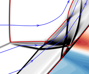
Since the outermost peak is much higher than the heating loads in the middle of the crotch area, it may damage the structure of vehicles. The flow details around the outermost peak (the red box in figure 7c) are magnified in figure 8. For a more precise analysis, the field is divided into several subzones according to the shock waves and SL. Three representative 2-D streamlines are appended. The free stream is defined as zone (0). The streamline-a from zone (0) crosses the MS to zone (1) and decelerates to subsonic. The DS and MS intersect at a triple point (TP). A transmitted shock (TS1) and SL are generated from the TP. Essentially, the local shock structure resembles Edney's type-III shock interaction. Streamlines-b and streamlines-c cross the DS to zone (2) (streamline-c has already crossed the DS in the far front). Then streamlines-b crosses TS1 to zone (3), and streamline-c crosses CS1 to zone (4). TS1 and CS1 cross each other to become TS2 and CS2, which is similar to Edney's type-I shock interaction. Subsequently, TS2 impinges on the wall and causes as SWBLI. The CS2 impinges on the SL and reflects as Prandtl–Meyer expansion waves (PMER). Note that the SL coincides with the sonic line, which is the dividing line between the supersonic jet and the subsonic flow.

Figure 8. Numerical schlieren around the outermost peak. The blue lines with arrows are 2-D streamlines and red lines are sonic lines (Ma = 1).
Details of the SWBLI region are shown in figure 9(a–c). The pressure contour and streamlines near the TS2 impingement (see figure 9a) show that TS2 causes a strong SWBLI with flow separation. The separation bubble footprint on the surface is visualized by limiting streamlines, as shown in figure 9(b). The convergent line on the left is a separation line (SepL), and the divergent line on the right is a reattachment line (RL). Note that the SWBLI region has a 3-D characteristic. The SepL and RL are curved due to the swept-back nature of TS2. Along the z-direction, the crossing flow increases and the heat flux decreases. However, the SWBLI is nominally 2-D near the centreline, since the limiting streamlines show that there is almost no crossing flow here. The centreline p and q distributions under the SWBLI region are shown in figure 9(c). The wall pressure experiences two increasing steps, which are caused by separation shock (SS) and reattachment shock (RS), respectively. There is a pressure plateau (pplt) under the separation bubble. The heat flux decreases in the separation region and then increases with the reattachment. The positions of ppeak and qpeak coincide. Downstream of the SWBLI region, both p and q decrease due to the favourable pressure gradient caused by the PMER.

Figure 9. Flow details around the SWBLI region: (a) pressure contour with 2-D streamlines; (b) wall heat flux with limiting streamlines; (c) pressure/heating loads on the centreline.
3.2. Modelling of shock interactions
The 3-D simulation result of VSBLE shows that the self-induced shock interactions cause transmitted shocks and extremely high heat flux peaks on the crotch. However, due to the complexity of the local shock structures, understanding the flow mechanism and predicting the heat flux peak are still challenging. It is necessary to develop a universal and effective model to solve the flow parameters of each subzone and predict the peak heat flux. Note that most of the flow field far from the wall can be regarded as inviscid shock–shock interactions. In the near-wall region, the viscous effect must be considered.
A simplified model is proposed to isolate the SWBLI region from the overall flow field by a control volume, which can be regarded as a black box. Outside the black box, inviscid shock relations (Rankin–Hugoniot relations) are used to solve the shock interactions. For the black box, boundary conditions obtained by the inviscid solutions are used as input variables. The output variables, including the SWBLI characteristics and pressure/heating peaks, can be predicted by a 2-D simplified simulation.
To make these ideas concrete, a 2-D inviscid shock interaction sketch (see figure 10a) is drawn to describe the structures in the schlieren (see figure 8b). Black dashed lines frame the SWBLI area as a black box. Some simplifications need to be explained: first, the details of the SWBLI are replaced by several inviscid shocks; second, the wall is regarded as a flat plate; furthermore, the MS is idealized as a normal shock without a deflection angle. Next, the regions outside and inside the black box are solved separately.

Figure 10. (a) The 2-D shock interaction sketch and (b) pressure–deflection angle shock polar. The thick blue lines represent shocks, the thin blue lines with arrows represent streamlines and the red double-dashed line represents the SL.
3.2.1. Inviscid analysis for the shock interactions
First, the flow field outside of the black box is analysed by inviscid theory. The classical theory of wave systems is listed in Appendix A. The parameters of each subzone are represented by their subscript. The deflection angle of flow across the shock is θ. Additionally, a pressure–deflection angle shock polar is plotted in figure 10(b) according to the Mach number of each subzone. The shock interactions are solved along the streamlines. As shown in figure 10(a), streamline-a from zone (0) crosses the normal shock MS to zone (1). The parameters of zone (1) can be calculated using the normal-shock relation:
 \begin{equation}Ma_1^2 = f(M{a_\infty },0),\quad {p_1}/{p_\infty } = g(M{a_\infty },0).\end{equation}
All states that may be reached from zone (0) by passing through any oblique/normal shock are represented by the polar  $\varGamma$0 in figure 10(b), which is plotted by the Mach number of the incoming flow. Since streamline-a crosses the MS without deflection, the strength of the MS is represented by the pressure jump between the origin and the apex of $\varGamma$0 where both ordinates are zero. As shown in figure 11, streamline-b from the free stream first crosses the oblique shock DS to zone (2). The shock angle (β 2) of the DS is equal to the half-span angle of the VSBLE, that is, β 2 = 24°. The deflection angle θ 2 of the DS can be solved by
 \begin{equation}S(M{a_\infty },{\beta _2},{\theta _2}) = 0.\end{equation}
The parameters of zone (2) can be calculated using the oblique shock relation:
 \begin{equation}Ma_2^2 = f(M{a_\infty },{\beta _2}),\quad {p_2}/{p_\infty } = g(M{a_\infty },{\beta _2}).\end{equation}
The polar  $\varGamma$2 of zone (2) is plotted according to Ma 2, and its origin is at the point (θ 2, p 2/p∞), which is the weak solution of $\varGamma$0. The strength of the DS is represented by the pressure jump from p∞ to p 2. Then the streamline-b crosses TS1 to zone (3). Zone (1) and zone (3) are connected by the SL. According to triple point theory, the pressure and flow direction on both sides of the SL are continuous. That is,
 \begin{equation}{p_1} = {p_3},\quad {\theta _1} = {\theta _2} + {\theta _3}.\end{equation}
Since θ 1 = 0, θ 3 = −θ 2. The shock angle β 3 of TS 1 is related to the deflection angle θ 3 by
 \begin{equation}S(M{a_\infty },{\beta _3},{\theta _3}) = 0.\end{equation}
The parameters of zone (3) can be calculated using the oblique shock relation:
 \begin{equation}Ma_3^2 = f(M{a_2},{\beta _3}),\quad {p_3}/{p_2} = g(M{a_2},{\beta _3}).\end{equation}
The polar  $\varGamma$3 of zone (3) can be plotted according to Ma 3, and its origin is at the point (0, p 3/p∞), which is the weak solution of $\varGamma$2. In addition, the origin of $\varGamma$3 also coincides with the apex of $\varGamma$0, because the static pressure of zone (1) and zone (3) is equal. The strength of TS1 is represented by the pressure jump from p 2 to p 3.

Figure 11. Shock interaction of the MS and DS.
As shown in figure 12, the parameters of zone (4) and zone (5) can be solved by flowing streamline-c. Note that the streamline-c has already crossed the DS in the far front although it is not shown here. The shock angle β 4 and deflection angle θ 4 of CS1 can be calculated by the theory proposed by Zhang (2021). The parameters of zone (4) can be calculated using the oblique shock relation:
 \begin{equation}Ma_4^2 = f(M{a_2},{\beta _4}),\quad {p_4}/{p_2} = g(M{a_2},{\beta _4}).\end{equation}
The polar  $\varGamma$4 of zone (4) is plotted by Ma 4. Its origin is at the point (θ 2+θ 4, p 4/p∞), which is the weak solution of $\varGamma$2. The strength of CS 1 is represented by the pressure jump from p 2 to p 4. TS1 and CS1 regularly reflect, which is similar to Edney's type-I shock interaction. Note that streamline-b passes through CS2 while streamline-c passes through TS2, and they are divided by the SL. Both sides of the SL have the same pressure and flow direction. The pressure and flow direction of zone (5) can be determined from the shock polar. That is, the intersection of $\varGamma$3 and $\varGamma$4 represents the state of zone (5). The strength of TS2 and CS2 are represented by the pressure jump from p 3 to p 5 and the pressure jump from p 4 to p 5, respectively.

Figure 12. Shock interaction of the TS1 and CS1.
The CS2 impinges the SL at P 2 and reflects as PMER. As shown in figure 13, streamline-b from zone (5) passes through the PMER to zone (6). And the pressure of zone (6) and zone (1) is equal. The deflection angle of the PMER can be solved by expansion wave relationship:
 \begin{equation}\upsilon (M{a_1}) - \upsilon (M{a_2}) = \theta ,\quad {p_6}/{p_5} = \chi (M{a_5},M{a_6}).\end{equation}
All the shock interactions outside the black box have been solved by the inviscid theory, and flow parameters of each sub-zone are listed in table 5.

Figure 13. Shock interaction of the CS2 and SL.
Table 5. Flow parameters of subzones.

3.2.2. Two-dimensional simulation of the black box
For the black box (the dashed line frame in figure 10a), the inlet condition on the left side has been solved by inviscid analysis. The incident shock wave TS2 and expansion wave PMER at the top are determined by their inviscid deflection angles. The boundaries at the bottom and right side are regarded as output interfaces. A simplified 2-D computational domain is constructed to simulate flow details in the black box. As shown in figure 14, TS2 and PMER are replaced by IS and PMEW, which are generated from a finite-length wedge. The wedge angle θw is the same as the TS 2 deflection angle. The incoming flow parameters are set by the zone (4) parameters in table 5. The boundary layer on the bottom is developed from a flat plate with a sharp leading edge. The distance from the leading edge to the shock impingement is the same as the length of the straight branches, to ensure that the boundary layer thickness is accurately reproduced. An outlet boundary condition is used on the right side. The geometric parameters of the 2-D computational domain are listed in table 6.

Figure 14. Two-dimensional computational domain for the black box.
Table 6. Two-dimensional computational domain geometric parameters.
Inviscid simulation is first conducted to clarify the shock structures, and the result is shown as a pressure contour in figure 15(a). In addition, the leading edge of the flat plate is not shown in the field. The IS and PMEW are generated from the leading edge and tail of the wedge, respectively. The PMEW first interacts with the IS from the same family and weakens the IS. Then the PMEW interacts with a reflected shock (RS) from the opposite families and penetrates the RS, causing a favourable pressure gradient in the near-wall region downstream of the shock impingement. The coordinate origin is set on the inviscid shock impingement.

Figure 15. Simulation results of the black box: (a) inviscid pressure contour and (b) numerical schlieren.
The viscous simulation result is shown as a numerical schlieren with the same perspective in figure 15(b), and a sonic line (the red line) is superimposed. The RS is replaced by the separation shock, reflected expansion wave and reattachment shock. The sonic line deviates from the wall near the shock impingement.
The SWBLI region is studied in detail to assess the accuracy of the heating/pressure peaks predicted by the model. The flow field is shown as the Mach contour, pressure contour and temperature contour in figure 16(a,b,e). The skin friction coefficient (Cf) is shown in figure 16(c). Furthermore, the p and q distributions on the wall are compared with the values on the VSBLE in figure 16(d,f). The p is normalized by the inflow static pressure p 4, and the temperature (T) is normalized by the inflow static temperature, T 4. The flow direction of the VSBLE uses the skin coordinate system (ξ) and is normalized by δ.

Figure 16. Simulation results of the SWBLI region: (a,b,e) Mach contour, pressure contour and temperature contour; (c) wall friction coefficient; (d,f) comparison of wall p/q between the 2-D model and the VSBLE.
Figures 16(a) and 16(c) shows that the Cf begins to decrease upstream of the separation shock. The length of the separation bubble is Lsep = 6.2δ, which is defined by the interval where Cf < 0. Downstream of the reattachment, Cf rises to a higher level than the incoming boundary layer. The reattached shear layer is accelerated by the PMEW and induces a higher wall shear stress.
Figure 16(d) shows that the pressure distribution predicted by the 2-D model is in good agreement with the VSBLE value. In particular, the plateau and peak are accurately reproduced. According to the free interaction theory, the strength of the separation shock only depends on the incoming boundary layer state and free stream Mach number. A plateau pressure prediction by Zukoski (Reference Zukoski1967) is shown in figure 16(d), which is in good agreement with the simulation result. This suggests that the Reynolds number is high enough such that the plateau pressure ratio essentially depends on the upstream Mach number, which is also observed by Pasquariello, Hickel & Adams (Reference Pasquariello, Hickel and Adams2017) in the direct numerical simulation results. The inviscid wall pressure is also shown in figure 16(d), and the peak value is much higher than the actual pressure. Because the subsonic layer can propagate the downstream favourable pressure gradient (caused by the PMEW) forwards, this indicates that viscosity is a non-negligible factor in SWBLI region.
Figure 16(e) shows a strong temperature gradient at the bottom of the incoming boundary layer. Figure 16(f) shows that the q slowly decreases with boundary layer thickening along the flow direction. In addition, the heat flux of a flat plate under the same inflow condition but without impinging shock is used as a reference. For the SWBLI region, the q first decreases with the flow separation then increases in the rear of the separation bubble. Furthermore, note that the pressure contour (see figure 16b) and temperature contour (see figure 16e) near the peak are similar to the distribution of stagnation points. Since the reattachment shock here is almost parallel to the wall, the shear layer normally passes through the shock with severe compression and heating, which causes extremely high pressure/heating loads. Such a flow pattern was also observed by Sriram et al. (Reference Sriram, Srinath, Devaraj and Jagadeesh2016).
As introduced in § 1, the pressure-heating correlation has a practical value for engineering. Markarian (Reference Markarian1968) summarized a simple correlation between the peak heat flux and peak pressure:
 \begin{equation}\frac{{q_{peak}^ \ast }}{{{q_{ref}}}} = C \times {\left( {\frac{{{p_{peak}}}}{{{p_{ref}}}}} \right)^N}.\end{equation}
In (3.9), C depends on the type of interactions and N depends on the incoming boundary layer state. According to the above analysis, the heat flux in the black box is essentially caused by an impinging shock wave/turbulence boundary layer interaction. For this classical SWBLI model, these parameters are defined as
 \begin{equation}C = 1,\quad N = 0.85.\end{equation}
The pref and qref are the wall pressure and heat flux of the incoming boundary layer, which can be obtained from the reference case (see figure 16f), where pref = p 4, qref = 3qo, and ppeak = 3.76p 4.
Therefore, the predicted peak heat flux is
 \begin{equation}q_{peak}^ \ast= 9.25{q_o},\end{equation}
which is only 0.5 % lower than the simulation result qpeak = 9.30qo. This result shows that the peaks of q and p on the VSBLE can be correlated by the classical pressure–heat flux correlation.
The comparison of the pressure/heating peak between the 2-D model prediction and the 3-D VSBLE is listed in table 7, and the prediction error is also shown. The model has a high prediction accuracy.
Table 7. Comparison of the p and q peaks between the 2-D model prediction and the VSBLE.

3.3. Shock control and 2-D SCB design
The above theoretical model proves that the high pressure/heating peak on the VSBLE is essentially caused by the incident shock. Inspired by this result, a local shock control strategy based on an SCB is proposed: try to weaken the pressure peak by controlling the incident shock, thereby indirectly reducing the heating loads. In this section, the control strategy and the SCB's parameter design are discussed first. A 2-D simulation for an oblique shock impinging on the SCB is then conducted to verify the control effect.
3.3.1. Discussion of the shock control strategy
As introduced in § 1, the SCB is a passive control device with a low-drag profile and good control effect. In particular, the concave-shaped SCB proposed by Schülein (2022) can split strong incident shock into a weaker multi-wave system, which has great potential to reduce the pressure/heating peaks. Inspired by the results of Schülein, a shock control strategy of placing a concave SCB on the shock impingement is proposed. However, Schülein also proves that the control effect is highly sensitive to the bump's contour shape and the relative position with the incident shock, which needs to be carefully designed to maximize the control performance.
Before choosing the shape parameters of the SCB, it should clarify two goals of our shock control strategy. On the one hand, we hope that the SCB can significantly reduce or even eliminate the wall pressure/heating peaks and the separation bubble caused by the incident shock. On the other hand, we hope that the SCB changes the original flow field as little as possible. Because the control strategy is designed for the inside of the black box (the near-wall region). If the shock interactions in the free stream change significantly, the position of the incident shock will also change, which may lead to control failure or bring additional high heating loads.
To achieve the first goal, an appropriate turning angle θE of EC (see figure 4a) needs to be selected, because the SCB essentially works through the beneficial interaction between incident shock and expansion fan generated by the EC. Schülein (2022) proved that the SCB had the best control effect when the θE was equal to or slightly greater than the incident shock deflection angle. In this paper, the deflection angle θw of the IS has been solved by the inviscid theory. Therefore, we need design the θE as θw. To achieve the second goal, a long and smooth CR should be designed to ensure that the incoming flow experiences an isentropic compression process without any shock. Therefore, an asymmetric SCB is adopted in our design to achieve both goals. Specifically, the contour shape of the CR is generated by a cubic spline (see (2.1)) with a leading-edge tangent to the mounting plane. The ER is a line with an incline angle of θc, which is equal to θw. The specific geometric parameters are listed in table 2.
Next, we focus on the position of the SCB. As shown in figure 17(a–c), flow patterns are divided into three cases according to the relative position of the EC and IS. In figure 17(a), the shock impingement is upstream of the EC, and neither the IS nor the RS is affected by the PMEEC. The SCB does not have a beneficial control effect in this case. In figure 17(b), the IS reflects at the EC, and the RS is weakened by PMEEC. In particular, if θE = θw, the RS will be eliminated theoretically. In figure 17(c), the shock impingement moves downstream of the EC. The IS first interacts with the PMEEC and reflects on the ER.

Figure 17. Shock structures near the SCB under different working conditions.
According to the three cases analysed by inviscid theory, the case in figure 17(b) seems to be the optimum working condition of the SCB. The pressure jump caused by the IS can be weakened or even eliminated by the EC. However, such a design may cause problems in applications. On the one hand, the SCB is under a thick boundary layer in viscous flow. The IS may cause a strong SWBLI on the impingement. Many studies (White & Ault Reference White and Ault1996; Li & Yang Reference Li and Yang2015; Sathia Narayanan & Verma Reference Sathia Narayanan and Verma2015; Zhang et al. Reference Zhang, Tong, Duan and Li2021b) on the SWBLI near an expansion corner show that if the IS impinges on the EC, the SWBLI-induced separation bubble will not be eliminated. The subsonic layer can propagate the adverse pressure gradient forwards. The boundary layer separates upstream of the EC and reattaches near the EC, which may induce a pressure/heating peak at the reattachment. On the other hand, it is too demanding to ensure that the IS impinges at the EC accurately. Experiments and simulations show that the transmitted shock (TS2) of the VSBLE has a minor amplitude oscillation mode. This means that if the shock impingement moves upstream of the EC, the bump will lose its control effects. Such a design may weaken the robustness of the SCB.
In fact, when the IS impinges the boundary layer at a short distance downstream of the EC (as seen in figure 17c), both the separation bubble and the pressure/heating loads will be reduced. Chew (Reference Chew1979) advised the designer to set the shock impingement about 3δ–4δ downstream of the expansion corner. Therefore, the bump's control mechanism for the case in figure 17(c) is the focus of subsequent study. The shock/expansion wave interactions around the expansion ramp are shown in detail by inviscid theory. In addition, the CR of the bump is simplified by a flat plate because  ${L_{CR}} \gg {L_{ER}}$, as shown in figure 4(b).
As shown in figure 18(a), the inviscid method proposed by Yao, Li & Wu (Reference Yao, Li and Wu2013) is adopted to solve the shock wave/expansion wave interactions near the SCB. The PMEEC is discretized into several Mach waves and interacts separately with the IS from the opposite families. The transmitted shock (IS’) is bent towards the wall. The join-generated shock (JS) is generated from the CC, where the bump and flat plate join. The flow field is divided into several subzones according to the wave system. Two streamlines with different distances from the wall are shown. The shock intensity and flow parameters of each subzone are solved following the streamlines, and a pressure–deflection angle shock polar is drawn to visualize the shock intensity (see figure 18b). The classical theory of wave systems is listed in Appendix A.

Figure 18. (a) Shock structures near the ER and (b) pressure–deflection angle shock polar.
Streamline-a from zone (0) crosses the IS with deflection angle θ 1, which is known. The shock angle β 1 is related to the deflection angle θ 1 by
 \begin{equation}S(M{a_\infty },{\beta _1},{\theta _1}) = 0.\end{equation}
The parameters of zone (1) can be solved using the oblique shock relation:
 \begin{equation}Ma_1^2 = f(M{a_\infty },{\beta _1}),\quad \frac{{{p_1}}}{{{p_\infty }}} = g(M{a_\infty },{\beta _1}).\end{equation}
Streamline-b first passes through the PMEEC with deflection angle α, which is known. The parameters of zone (2) can be solved by Prandtl–Meyer function:
 \begin{equation}\upsilon (M{a_\infty }) - \upsilon (M{a_2}) = \alpha ,\quad \frac{{{p_2}}}{{{p_\infty }}} = \chi (M{a_\infty },M{a_2}),\quad \frac{{\rho _2^\gamma }}{{\rho _\infty ^\gamma }} = \frac{{{p_2}}}{{{p_\infty }}}.\end{equation}
The IS interacts with the PMEEC from the opposite families and penetrate each other to become the transmitted shock IS’ and transmitted wave PMEEC’. To simplify the analysis, the PMEEC is discretized into several Mach waves, and each Mach wave interacts with the IS separately. Figure 19 is a schematic diagram of the interaction between a Mach wave and IS. The flow parameters of zone (1) and zone (2) have been solved. Streamline-a from zone (1) crosses PMEEC’ to zone (3a) with a deflection angle θ 3a. The parameters of zone (3a) can be solved by Prandtl–Meyer function:
 \begin{equation}\upsilon (M{a_1}) - \upsilon (M{a_{3a}}) = {\theta _{3a}},\quad \frac{{{p_{3a}}}}{{{p_1}}} = \chi (M{a_1},M{a_{3a}}).\end{equation}
Streamline-b from zone (2) crosses IS’ to zone (3b) with deflection angle θ 3b. The parameters of zone (3b) can be solved using the oblique shock relation:
 \begin{equation}Ma_{3b}^2 = f(M{a_2},{\beta _{3b}}),\quad \frac{{{p_{3b}}}}{{{p_2}}} = g(M{a_2},{\beta _{3b}}),\quad S(M{a_2},{\beta _{3b}},{\theta _{3b}}) = 0.\end{equation}
A slipline divides zone (3a) and zone (3b). The following relations must hold:
 \begin{equation}{p_{3a}} = {p_{3b}},\quad {\theta _1} + {\theta _{3a}} = {\theta _2} + {\theta _{3b}}.\end{equation}
By combining the equations (3.15), (3.16) and (3.17), the shock/expansion wave interaction can be solved.

Figure 19. Shock/Mach wave interaction of the IS and PMEEC.
Next, streamline-b from zone (3b) crosses the RS to zone (4) with deflection angle θ 4. As shown in figure 18(a), the flow directions of zone (2) and zone (4) are parallel to the wall (ER). The following relation must hold:
 \begin{equation}{\theta _3} = {\theta _4}.\end{equation}
The parameters of zone (4) can be solved using the oblique shock relation:
 \begin{equation}Ma_4^2 = f(M{a_{3b}},{\beta _4}),\quad \frac{{{p_4}}}{{{p_3}}} = g(M{a_{3b}},{\beta _4}),\quad S(M{a_{3b}},{\beta _4},{\theta _4}) = 0.\end{equation}
Finally, streamline-b from zone (4) crosses the JS to zone (5) with deflection angle θ 5, which is the same as the turning angle of the CC. There is θ 5 = α. The parameters of zone (5) can be calculated using the oblique shock relation:
 \begin{equation}Ma_5^2 = f(M{a_4},{\beta _5}),\quad \frac{{{p_5}}}{{{p_4}}} = g(M{a_4},{\beta _5}),\quad S(M{a_4},{\beta _5},{\theta _5}) = 0.\end{equation}
The pressure–deflection angle shock polars  $\varGamma$2, $\varGamma$3 and $\varGamma$4 are plotted by the Mach number of zone (2), zone (3) and zone (4), respectively. The shock intensities of the IS, RS and JS are represented by their pressure jumps. The flow parameters of each subzone are listed in table 8.
Table 8. Flow parameters of subzones.

The inviscid theoretical analysis shows that the SCB splits the incident shock into a multiwave system, but also has some adverse effects. On the one hand, although the peak pressure (p 4) at the IS impingement is reduced, the local pressure jump (p 4/p 2) is increased. This may cause a larger separation bubble in viscous flow. On the other hand, the pressure (p 5) after the JS is higher, which may cause a new heating/pressure peak downstream of the SCB. However, it should be noted that the PMEW from the wedge tail was ignored in the above analysis to simplify the calculation. In fact, the PMEW will not only weaken the intensity of incident shock but also induce a favourable pressure gradient in the near wall region.
3.3.2. Two-dimensional simulations of SCB
To quantitatively evaluate the control effect of the SCB with an incident shock, a 2-D simulation is conducted using inviscid and viscous methods. The free stream parameters are set by the inflow condition of the black box (the zone (4) parameters in table 5). The computational domain is similar to the baseline black box (see figure 14), except the flat plate at the bottom is replaced by an expansion/compression corner configuration (see figure 4b). The coordinate origin is set on the EC. Both x and y are normalized by the incoming boundary layer thickness δ.
Inviscid simulation is first conducted and the result is shown as a pressure contour in figure 20(a). The IS first interacts with the PMEW from the same family, then interacts with the PMEEC from the opposite families, and reflects on the ER at x = 3.81δ. Note that the PMEW penetrates the RS and JS successively and causes a favourable pressure gradient in the near-wall region.

Figure 20. Simulation results of the 2-D SCB: (a) inviscid pressure contour and (b) numerical schlieren.
The viscous simulation result is shown in numerical schlieren (see figure 20b) and a sonic line is superimposed. Behind the EC, the sonic line significantly deviates from the wall, indicating that the IS causes a strong SWBLI with flow separation. The SWBLI near the CC is weaker because the JS is similar to the inviscid shock.
The p and q distributions on the SCB are shown in figure 21(a,b) and compared with the values of the baseline case. The original single peak is split into double peaks by the SCB, and the pressure/heating loads on the SCB are significantly reduced.

Figure 21. (a) Pressure and (b) heat flux distributions at the bottom of the black box with/without the SCB.
As shown in the schlieren (see figure 20b), the key feature of the flow around the SCB is the SWBLI caused by the IS and JS. To further explore the SCB control mechanism in viscous flow, details around the two SWBLI regions are shown with schlieren, Mach contours and pressure contours in figure 22(a–h); moreover, the distribution of Cf and p on the surface are also extracted and shown with lines in figure 22(e,f,i,j).

Figure 22. Simulation results of the SWBLI regions: (a,b) numerical schlieren; (c,d) Mach contours; (e,f) wall friction coefficient; (g,h) pressure contours; (i,j) wall pressure distributions.
The IS-induced SWBLI region is analysed first. The schlieren (see figure 22a) shows that supersonic flow above the sonic line passes through the PMEEC, SS, IS’, reflected PME and RS from left to right. The subsonic separation bubble is located behind the EC, and the separation length is Lsep = 3.2δ (see figure 22e). Figures 22(g) and 22(i) show that the wall pressure first decreases at the EC, then experiences two increasing steps, successively caused by the SS and the RS, and reaches a maximum (pmax = 1.58p∞) downstream of the reattachment point at x = 5.0δ. The SWBLI caused by the JS is relatively weaker. The schlieren (see figure 22b) shows that the JS is converged by a series of compression waves from the sonic line. The length of separation bubble is only 0.32δ (see figure 22f). Figure 22(j) shows that there is no obvious plateau during the wall pressure rising. The local pressure peak  $({p^{\prime}_{max}} = 1.56{p_\infty })$ is located downstream of the CC at x = 15.2δ.
It should be noted that the weakening of the two pressure peaks is consistent with the prediction in the inviscid analysis, and we refer to this control mechanism of the SCB as the inviscid effect. However, the SWBLI-induced separation bubbles are also suppressed, which is beyond expectation. Because the inviscid analysis shows that the IS’ causes a higher pressure jump at the impingement, which may induce a larger separation bubble. This result seems to contradict the viscous simulation results. In fact, the SWBLI-induced separation depends not only on the shock intensity but also on the state of incoming boundary layer (Pirozzoli & Grasso Reference Pirozzoli and Grasso2006). This means that the SCB may have affected the boundary layer upstream of the SWBLI regions.
The flow field is refocused. In the schlieren (see figure 22a), the sonic line seems to be closer to the surface at the EC. The Mach contour (see figure 22c) at the bottom of the boundary layer is also changed by the EC. In addition, upstream of both SWBLI regions, Cf has a higher level than the incoming boundary layer (see figures 22e and 22f).
Studies (Giepman, Schrijer & van Oudheusden Reference Giepman, Schrijer and van Oudheusden2014) show that the SWBLI-induced separation bubble is sensitive to the low-momentum gas at the bottom of the incoming boundary layer. Therefore, the near-wall region (y < 0.1δ) Mach profiles upstream of the IS impingement (at x = 0) and the JS impingement (at x = 12δ) are extracted and shown in figure 23(a,b). For comparison, the Mach profile of the undisturbed incoming boundary layer (at x = −δ) is superimposed. The positions of the three stations are marked by dashed lines in figure 20(b). Moreover, the sonic line height (yMa = 1), the boundary layer incompressible shape factor (Hi) and the separation length are listed in table 9. The Hi is defined by
 \begin{equation}{H_i} = \frac{{\delta _i^\ast }}{{{\theta _i}}},\end{equation}
where δi* is the incompressible displacement thickness and θi is the momentum thickness. They are defined by
 \begin{equation}\delta _i^\ast= \int_0^\delta {\left( {1 - \frac{u}{{{u_e}}}} \right)\,\textrm{d}y} ,\quad {\theta _i} = \int_0^\delta {\frac{u}{{{u_e}}}\left( {1 - \frac{u}{{{u_e}}}} \right)\,\textrm{d}y} .\end{equation}
Figure 23(a,b) and table 9 show that both the stations of x = 0 and x = 12δ have fuller Mach profiles, thinner subsonic layers and lower shape factors than the reference boundary layer. This change in the boundary layer can be explained from figure 22(g). The local favourable pressure gradient induced by the PMEEC propagates forwards along the subsonic layer. The low-momentum gas at the bottom of the boundary layer accelerates in front of the EC, which induces a higher wall shear stress and a thinner subsonic layer.

Figure 23. Mach profiles of different stations.
Table 9. Comparison of boundary layer state between different stations.

This change in the boundary layer may have two effects on the SWBLI regions. On the one hand, the higher-momentum gas in the near-wall region has a stronger ability to resist separation. On the other hand, the thinner subsonic layers hinder the propagation of the downstream adverse pressure gradient. Therefore, although the local pressure jump is higher, the separation bubble is smaller (see table 9). We call this SCB control mechanism the viscous effect.
3.4. Simulation of the VSBLE with SCBs
The preliminary design of the SCB in the section above is completed in the black box using a 2-D method. However, in practical applications, the SCB may be under off-design conditions due to the swept shock or crossing flow. In this section, the SCB is placed on the VSBLE to examine its actual performance. The schematic of the VSBLE with SCBs have been shown in figure 4(c). The position of the EC is determined by the incident shock TS2, ensuring that the shock impingement is approximately 3δ–4δ downstream of the EC.
A 3-D simulation for the VSBLE with SCBs is conducted with an incoming flow condition the same as the baseline VSBLE (see table 4). Mach contour and numerical schlieren of crotch area are shown in figures 24(a) and 24(c), and the wall is coloured by heat flux contour. The heat flux and pressure distributions along the centreline are shown in figures 24(b) and 24(d). The main flow structures in the crotch area, including the MS, CVP and supersonic jets are similar to the structures of the baseline VSBLE. It should be noted that the outermost heat flux peak is reduced by 66 %, and the pressure peak is reduced by 58 %. This indicates that the SCB plays a good control role and does not change the main flow structures.

Figure 24. Simulation results of VSBLE with SCBs: (a) Mach contour and (c) numerical schlieren of the crotch area; (b) heat flux and (d) pressure distribution along the centreline. The red solid lines represent the VSBLE with SCBs and the blue dash–dotted lines represent the baseline VSBLE.
To further explore the 3-D flow details around the SCB, figure 25(a–c) shows the heat flux contour and limiting streamlines on the SCB. As seen from the limiting streamlines, the flow pattern on the bump changed significantly along the z direction. The heat flux peak is located at approximately z/r = 1/2, not at the centreline. Furthermore, four typical slices from z/r = 0 to z/r = 1/2 are extracted and shown as numerical schlieren (see figure 26a–d), to evaluate the control effect of the SCB under various working conditions.

Figure 25. Heat flux and limiting streamlines of the SCB: (a) a global view; (b,c) details near z/r = 1/2 and z/r = 0. The SL is the separation line, the RL is the reattachment line, the pink dashed lines represent the EC and CC contours of the SCB, and the green dash–dotted lines represent different z slices.

Figure 26. Numerical schlieren of different z slices and wall heat flux.
As seen from the limiting streamlines between z/r = 0 and z/r = 1/4 in figure 25(c), the flow pattern is nominally two-dimensional. The SL is located a short distance downstream of the EC. The RL is near and parallel to the SL. The SWBLI-induced separation bubble is suppressed by the SCB around the centreline. The local heat flux is also kept at a lower level. As seen from the schlieren, the shock structures at z/r = 0 (see figure 26a) and z/r = 1/4 (see figure 26b) are consistent with the 2-D simulation result (see figure 20b), indicating that the SCB is under the design condition. In addition, due to the incident shock (TS2) sweeping back along the z-direction, the shock impingement in the z/r = 1/4 slice moves slightly downstream.
However, the flow pattern changes significantly at z/r = 3/8. Figure 25(a) shows that the RL deviates from the SL and is located on the CC. Furthermore, the heat flux downstream of the CC shows an increasing trend. Schlieren of the slice z/r = 3/8 (see figure 26c) shows that the TS2 impingement is close to the CC. The RS interacts with the JS to form a λ structure above the CC. The global heat flux peak is located at the slice z/r = 1/2. Figure 25(b) shows that the SL is still upstream of the CC, while the RL is downstream of the CC. Schlieren of the slice z/r = 1/2 (see figure 26d) shows that the TS2 nominal impingement is located at the CC, and there is a large separation bubble above the CC. The JS is replaced by a stronger reattachment shock, which causes a new heat flux peak downstream of the RL (see figure 25b). For the region z/r > 1/2, the limiting streamlines (see figure 25a) show that the crossing flow becomes dominant. The TS2 intensity is significantly weakened due to its sweeping back. The local heat flux also decreases.
To quantitatively evaluate the robustness of the SCB, q and p distributions on the SCB at z/r = 0 and z/r = 1/2 are extracted and shown in figure 27(a,b), and the baseline VSBLE values are superimposed as references. The q and p distributions at the slice z/r = 0 are similar to the 2-D simulation results of the SCB in figure 21(a,b). The original single peak is split by the SCB into double peaks, and both peaks are significantly weakened. For the slice z/r = 1/2, the p experiences two increasing steps caused by the SS and RS respectively, and the q first decreases with the flow separation and then increases with the reattachment. Both the p and q peaks are located downstream of the CC. The peak values are listed in table 10. The q peak of the slice z/r = 1/2 is higher than that of the slice z = 0 but is much lower than the baseline value.

Figure 27. Comparison of (a) heat flux and (b) pressure distribution of different slices on the VSBLE with SCBs and the baseline VSBLE.
Table 10. Heating and pressure peaks of the VSBLE with SCBs and the baseline VSBLE.

In summary, the optimal control effect of the SCB is around the centreline (0 ≤ z/r < 1/4). Both the separation length and the heat flux are suppressed at a lower level. With the incident shock swept back, the SCB starts to deviate from the design condition at z/r = 3/8 and reaches the most unfavourable condition at z/r = 1/2. However, although the SCB's control effect under off-design conditions is weakened, both the heat flux and pressure peaks are still significantly reduced compared to the baseline peaks.
4. Conclusions
Hypersonic flow on the baseline VSBLE model with R/r = 3.25 at Mach 12 is numerically investigated. Complex flow structures including the supersonic jet, Mach reflection, shock interactions and SWBLI in the crotch area are found. In particular, the transmitted shock impinging on the boundary layer causes extremely high heat flux peaks that can be up to 9.3qo. Based on the shock structures, a simplified model is proposed to isolate the SWBLI region from the overall flow field by a control volume, which can be regarded as a black box. Outside the black box, the shock interactions and flow parameters of each subzone are solved by inviscid shock relations. For the black box, the SWBLI characteristics and the pressure/heating peak can be predicted by 2-D simulation with high accuracy. Additionally, the pressure peak and heat flux peak are correlated by classical formulae. The model provides an idea for the simplified solution of complex shock interactions.
Furthermore, a local shock control strategy based on an SCB is discussed. The purpose is to weaken the pressure peak by controlling the incident shock, thereby indirectly reducing the heating loads. The relative positions between the SCB and the incident shock are first analysed by inviscid theory, and it is found that when the incident shock impinges 3δ–4δ downstream of EC, the SCB is under the best-design condition. Moreover, the control mechanism is studied by numerical simulations. The results show that the SCB has two effects on the SWBLI regions. On the one hand, the SCB splits the incident shock into a weaker multi-wave system and significantly reduces the pressure/heating loads on the shock impingement by the inviscid effect. On the other hand, the SCB changes the Mach profile of the incoming boundary layer and suppresses the SWBLI-induced separation bubble by the viscous effect.
Finally, the VSBLE with SCBs is numerically investigated and compared with the baseline VSBLE. The result shows that the SCB reduced the heat flux peak by 66 % and suppressed the SWBLI-induced separation around the centreline. The SCB is less effective at z/r = 1/2 due to the incident shock swept back; although there is only a small increase in heating load, this heating load is far below the baseline peak heat flux. This provides a direction for further SCB optimization, that is, if the shape of the SCB can be designed according to the three-dimensional swept shock, its control effect may be better. In this paper, the SCB is first applied to hypersonic flow as a thermal protection device, and its great potential in heating reduction is demonstrated.
Funding
This study was supported by grants from the National Natural Science Foundation of China (grant no. 92252201).
Declaration of interests
The authors report no conflict of interest.
Appendix A. Oblique shock wave and expansion wave relationships
The classical theory of wave systems is briefly listed (Yao et al. Reference Yao, Li and Wu2013). The parameters upstream and downstream of the wave are represented by subscript ‘0’ and ‘1’. The deflection angle of flow across the shock or expansion wave is θ. For flow across oblique shocks,
 \begin{equation}\left. {\begin{array}{*{20}{c@{}}} {Ma_1^2 = f(M{a_0},{\beta_1}),\quad \dfrac{{{p_1}}}{{{p_0}}} = g(M{a_0},{\beta_1}),\quad \dfrac{{{\rho_1}}}{{{\rho_0}}} = h(M{a_0},{\beta_1})}\\ {\dfrac{{{a_1}}}{{{a_0}}} = A(M{a_0},{\beta_1}),\quad S(M{a_0},{\beta_1},{\theta_1}) = 0} \end{array}} \right\},\end{equation}
where
 \begin{gather}f(Ma,\beta ) = \frac{{M{a^2} + \dfrac{2}{{\gamma - 1}}}}{{\dfrac{{2\gamma }}{{\gamma - 1}}M{a^2}{{\sin }^2}\beta - 1}} + \dfrac{{M{a^2}{{\cos }^2}\beta }}{{\dfrac{{\gamma - 1}}{2}M{a^2}{{\sin }^2}\beta + 1}},\end{gather}
 \begin{gather}g(Ma,\beta ) = \frac{{2\gamma }}{{\gamma + 1}}M{a^2}{\sin ^2}\beta - \frac{{\gamma - 1}}{{\gamma + 1}},\end{gather}
 \begin{gather}h(Ma,\beta ) = \frac{{(\gamma + 1)M{a^2}{{\sin }^2}\beta }}{{(\gamma - 1)M{a^2}{{\sin }^2}\beta + 2}},\end{gather}
 \begin{gather}A(Ma,\beta ) = \frac{{{{[(\gamma - 1)M{a^2}{{\sin }^2}\beta + 2]}^{{1 / 2}}}{{[2\gamma M{a^2}{{\sin }^2}\beta - (\gamma - 1)]}^{{1 / 2}}}}}{{(\gamma + 1)Ma\sin \beta }},\end{gather}
 \begin{gather}S(Ma,\beta ,\theta ) = 2\cot \beta \frac{{M{a^2}{{\sin }^2}\beta - 1}}{{M{a^2}(\gamma + \cos 2\beta ) + 2}} - \tan \theta .\end{gather}
The relationship for the expansion wave is
 \begin{equation}\upsilon (M{a_0}) - \upsilon (M{a_1}) = \theta ,\quad \frac{{{p_1}}}{{{p_0}}} = \chi (M{a_0},M{a_1}),\quad \frac{{\rho _1^\gamma }}{{\rho _0^\gamma }} = \frac{{{p_1}}}{{{p_0}}},\end{equation}
here, the ν(M) is Prandtl–Meyer relationship:
 \begin{equation}\upsilon (M) = \sqrt {\frac{{\gamma + 1}}{{\gamma - 1}}} {\tan ^{ - 1}}\sqrt {\frac{{\gamma + 1}}{{\gamma - 1}}(M{a^2} - 1)} - {\tan ^{ - 1}}\sqrt {M{a^2} - 1} .\end{equation}
Additionally,
 \begin{equation}\chi (M{a_0}M{a_1}) = {\left( {\frac{{2 + (\gamma - 1)Ma_0^2}}{{2 + (\gamma - 1)Ma_1^2}}} \right)^{\gamma /(\gamma - 1)}}.\end{equation}


