Laser profiler characteristics

To obtain typical values for/, we consider a particular laser profiler, the “Geodolite 3A” which has been extensively used in sea-ice reconnaissance (see for example Reference KetchumKetchum, 1971) and also in land applications (Link, f 1970]). This system is a typical continuous-wave laser profiler. Range measurements are accomplished through a phase comparison between the laser beam (with a modulated wave superimposed) directed at the terrain and the reflected light from the terrain. This phase difference is used to create a square wave with the tooth width proportional to the distance to the terrain surface modulo the superimposed wavelength (i.e. the tooth width is proportional to the distance less an integral number of wavelengths). This square wave is run through a simple integrating circuit whose output is an analog signal. The integrating circuit smooths out distance errors (due to varying tooth widths) but has a finite response time and thus massages the high-frequency components. The response time is usually variable so one can trade off error reduction for a faster response time and vice versa. The available response limes for the Geodolite 3Λ (defined as a 95% response to a step input) include 1, 2, 5, 10, 20, 50 and 100 ms. The modulation frequency is normally selected so that the phase delay of the reflected signal is one wavelength for a desired range change of 10 ft or 10 m depending on the particular instrument. Longer wavelengths may be chosen but they decrease accuracy. When this range interval is exceeded the indicated distance jumps back to zero and starts again. Such jumps are referred to as phase shifts.

Besides the range analog voltage, signal outputs from the laser include the photomultiplier output (return signal amplitude), which provides a means of distinguishing open-water areas from ice (when flying over lakes or sea ice) since signal return is quite low from open water.

Initial processing of the data involves removal of the phase shifts. The typical procedure is to digitize the analog signal at some high rate (200 samples per second) and then use simple algorithms to remove the phase shifts. Unfortunately phase discontinuities (range measurement errors caused by momentary loss of signal return) also occur occasionally. Such discontinuities are of varying magnitudes and usually require visual examination for identification and correction. The treatment of these kinds of instrumental peculiarities, although sometimes bothersome, is essentially a software problem which we will not discuss in further detail here. Additional discussion of this problem is given by Reference Mock, Mock, Hartwell and HiblerMock and others (1974).

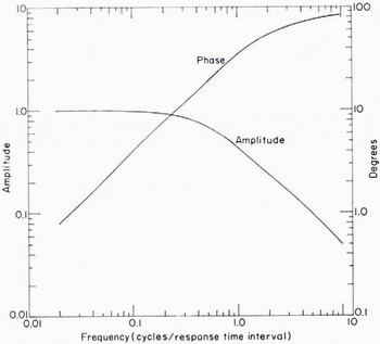
Fig. 1. Amplitude and phase of a causal exponential response function. The response time is defined as the time for a 95% response to a step input. Positive phase angles correspond to the output signal lagging behind the input signal

Once the data is in an acceptable form with phase shift and discontinuities removed, we may examine how the response messages the data. Since the integrating circuit has essentially an exponential response, its frequency response F(W) may be calculated straightforwardly:

(1)

where by definition of the 95% response time Δt, β = —In (0.05)/Δt. In Fig. 1 we give a plot of the amplitude and phase of this response function with a positive phase angle indicating that the output signal is lagging in time behind the input. For conversion to distance, we note that 100 m/s (194.4 knots) is a typical aircraft speed, so that 10 ms corresponds to a 1 m distance. As can be seen from the figure, the high-frequency cut-off f₂ , below which the data is modified little, is approximately 0.25 cycles/Δt. For a 10 ms response time and an aircraft speed of 100 m/s, this corresponds to a 4 m wavelength. This cut-off is close to the empirical wavelength cut-off of 6 m found by Reference Tooma and TuckerTooma and Tucker (1973) in a comparison of laser-sea-ice profiles with aerial stereophotogrammetric profiles.

Fig. 2. Results of filtering a simulated terrain profile with a causal exponential response function. An tiircraft speed of 100 m/s (194.4 knots) was assumed. The. noise was obtained by applying the various exponential filters to a fixed gaussian white-noise time series.

To examine the smoothing of the terrain profile by the profilometer plus the effect of noise more directly it is useful to filter some simulated terrain with exponential filters. The results of such a simulation are shown in Fig. 2 where we have simulated a terrain by using a first-order Markovian process. Such a process has been found to have similar spectral characteristics to sea-ice profiles.

A nominal aircraft speed of 100 m/s is assumed. For the noise signal we used the fact that typical errors in sea-ice profiles (obtained by looking at the profile on flat ice) are of the order of 10 cm at a 10 ms response time (see for example Ketchum 1971, Reference LeSchack, LeSchack, Hibler and MorseLeSchack and others, unpublished). These errors are somewhat smaller than the errors obtained from laser profile tests over land (Link, [1970]), which is to be expected because of the poor reflectivity over land.

As can be seen from the figure, the 5 ms and 10 ms responses modify the terrain only slightly, whereas the 20 ms smoothing begins to change phases and amplitudes significantly. The noise level on the other hand is moderately higher for the 5 ms response time, suggesting that 10 ms is a good compromise. We note that the effect of instrument response time on noise levels was studied empirically by Link ([1970]) with results similar to the simulation in Fig. 2.

To summarize, the higher-frequency cut-off f₂ corresponds to wavelengths of the order of 2 to 4 m. Consequently, we may say that terrain that can be well described by samples every 1 or 2 m with height accuracy of few centimeters can be well characterized by aircraft profilometry. For more accuracy or a denser sampling rate, aircraft flying at speeds slower than c. 100 m/s would be needed. The price for this slower speed is a change in the low-frequency limit f₁ , as discussed next.

Aircraft motion treatment

The variation of the altitude and attitude of the aircraft cause spurious low-frequency components to be present in the profile. Examples of this effect are shown in Fig. 3 where two typical laser profile traces of sea ice are illustrated. The solid line is the estimated aircraft motion obtained according to a three-step digital filtering process discussed later (Reference HiblerHibler, 1972). The relevant observation here is that the aircraft motion causes variations of the order of 10 to 30 m with wavelengths greater than several hundred meters.

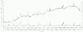
Fig. 3. Laser profile (curve a) of sea ice. Curve b represents the estimated variation in distance from the laser to the ice surface due to variation in aircraft altitude and attitude, arid curve c is the result of subtracting b from a.

Various hardware devices have been proposed to handle the aircraft motion. The most common suggestions have been to use cither a pressure-port calibrator and/or an accelerometer. The pressure-port method, although sensitive enough to resolve c. 0.15 m changes (Ketchum, 1971), is not highly useful because of horizontal variations in atmospheric pressure. To illustrate how great a problem this is, we note that vertical atmospheric changes are approximately 0.10 mbar/m (Reference Berry, Berry, Bollay and BeersBerry and others, 1945). For an estimate of horizontal pressure differences we calculated r.m.s. pressure differences between the three 1972 AIDJEX satellite stations located approximately 100 km apart, using pressure data reported by Reference ThorndikeThorndike and others (1972). For a 30 d period the r.m.s. differences averaged 0.016 mbar/km. This yields a height error of 0.16 m/km due to horizontal pressure variation, which is rather large especially for profiling Arctic sea ice.

The use of accelerometers appears to offer more promise although investigation of such data (personal communication from R. T. Lowry) indicates that they tend to drift slowly in time and thus cannot be used for the removal of extremely low-frequency height variations. A more complete discussion of the use of such data is given by Reference LowryLowry (1975).

However, even if the aircraft altitude could be determined exactly, there still remains the problem of roll and pitch which also change the range to the terrain surface. For example a roll of 1° at a 320 m altitude causes a range change of c. 0.09 m. This sort of problem can be handled by using a gyro-stabilized gimbel mount but such systems are rarely employed.

Because of these difficulties it is more common to use digital filtering techniques. For purposes of spectral calculations one can simply use a variety of high-pass filtering techniques (see for example Hibler and LeSchack, 1972). Such a procedure is effective (and necessary) in preventing “leakage” of the low-frequency spectral components to higher frequencies. However, for other purposes such a procedure is not entirely adequate. This is because there is an overlap between the surface roughness spectrum and the aircraft motion spectrum. This overlap is especially troublesome in sea-ice profiles in that, as a consequence of the overlap, a high-pass filter tends to depress the height of high ridges.

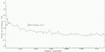
Fig. 4. Power spectra of the filtered and unfiltered profiles shown in Fig. 3. Curve a is the unfiltered profile spectrum, and curve b is the spectrum of the profile after removal of aircraft motion

To bypass this problem in sea ice a straight-forward three-step digital filtering process was developed by Hibler (1972). The technique consists of the following steps: (1) A symmetric high-pass convolution filter is applied to the initial profile. (2) From the filtered profile a set of minimum points are recorded; these minimum points are linearly interpolated and then (3) low-pass filtered to obtain an estimate of the aircraft motion. The aircraft motion is then subtracted from the initial profile and the resulting profile used for further analysis. The basis for this process is that the pack-ice surface profile is essentially a one-sided noise trace in that the roughness always rises up approximately from the water level. An example of this process is the smooth curve in Fig. 3 which, as can be seen, provides an aircraft motion curve which is very close to what would be estimated visually.

It is also instructive to compare the low-frequency portion of the spectrum of the unfiltered profile and the profile with the aircraft motion removed. In Fig. 4 we see such spectra corresponding to the profiles in Fig. 3. The spectra clearly indicate the problem of spectral overlap. Although approximately 99% of the low-frequency variance is due to the aircraft motion, the residual 1% is significant on the scale of surface roughness. The spectra also indicate that the cut-off at which the unprocessed spectrum merges with the filtered spectrum occurs at a wavelength of about 240 m. This indicates that although the aircraft motion has most of its variance at very low frequencies, it also has a significant portion (on the surface roughness scale) at higher frequencies.

To summarize, for speeds of the order of 100 m/s, aircraft motion directly affects the spectrum at wavelengths larger than c. 300 m. If the profile is to be used to examine variation in roughness at wavelengths less than 300 m, the data may be used directly simply by low-pass filtering. If not, then some subterfuge must be used to push back the cut-off to lower frequencies. Also speeds faster or slower than 100 m/s will tend to move the f₁ cut-off lower or higher respectively.

Classification of sea-ice ridging

Sea-ice ridges are an important deformation characteristic of the Arctic ice pack and have been actively studied in the past several years. Results of this work have included studies of the morphological characteristics of ridges (Reference Weeks, Weeks, Kovacs, Hibler, Wetteland and BruunWeeks and others, [1972]; Reference Kovacs and KarlssonKovacs, 1972), the development of mechanical ridge-formation models (Reference Parmerter and CoonParmerter and Coon, 1972); and the development of statistical models for describing the height and spatial distribution of pressure ridges (Hibler and others, 1972; Hibler and others, 1974). Laser profiles, in conjunction with the three-step filtering process, provide a means of rapidly compiling ridge height and spacing statistics along a straight-line path. Submarine sonar data, such as those discussed by Reference SwithinbankSwithinbank (1972), provide similar information on the distribution of ridge keel depths. Such straight-line distribution data is especially useful in sea ice since it appears that over reasonably large areas (tens of kilometres) ridges are close to being randomly oriented in direction (Mock and others, 1972). Consequently the total length of ridges per unit area is related to the number of ridges encountered per unit length along a straight-line path.

In order to reduce the number of parameters needed to describe ridging statistically it is useful to develop height and spacing distribution models. Such a reduction is especially important when large quantities of data are being processed and it is desired to examine spatial and temporal variations in ridging. To derive a model for ridge height distributions Hibler and others (1972) carried out a variational calculation in which the most probable arrangement of a given number of ridges for a given amount of deformed ice (with no restriction placed on the maximum ridge height) was derived. The result in general form is given by:

(2)

where P(H) dH is the probability of finding a ridge with height between H and H+dH, and λ and B(H) are to be determined. As a first approximation B(H) was simply assumed to be constant for H greater than some cut-off height h, a procedure which was found to yield adequate agreement with data above height h. Under this assumption Equation (2), when normalized to t for ridges above height h, becomes

(3)

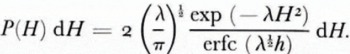
The key contribution of the variational calculation is the exp ( — λH²) term in Equation (2). Additional assumptions can be made in the variational calculation that justify taking B(H) as a constant (this was in fact done in the original paper by Hibler and others (1972)) but they tend to be oracular in nature. It is probably better to simply say that B(H) being constant for H > h is an empirical assumption that works reasonably well. A more detailed investigation with B(H) varying as a function of height (or depth) could well be a subject for further research.

To illustrate the fit of Equation (3) as well as geographical variation in ridging, we show in Fig. 5 three height distributions varying from heavily ridged ice near the northern Canadian Archipelago, to medium ridged ice near the North Pole and to lightly ridged ice in the Beaufort Sea. Each set of data was obtained from a laser track, c. 40 km in length, with data spacings of 1.2 m to 1.5 m depending on the average aircraft speed. The total number of ridges above 4 ft (1.22 m) in each 40 km track varied from c. 80 to c. 400 ridges. Ridges were digitally identified by declaring a profile peak to be a ridge when the peak is at least 2 ft (0.61 m) above minimum points located both right and left of the peak. Seventy-eight other-such 40 km samples have been fitted with Equation (3) with good agreement (Hibler and others, 1974).

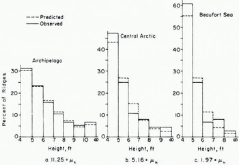
Fig. 5. Ridge height distributions taken in February 1973. Each distribution was taken from a laser track approximately 40 km in length and the average number of ridges per kilometer above 4 ft (1.22 m) is denoted by μ_h for each distribution. The two-parameter fit is indicated by dashed lines with the actual data being solid. Distribution a, was observed at approximately lat. 83° N., long. 85° W., b at lat. 87° N., long. 162° W., c at lat. 70° N., long. 139° W. The mean ridge heights for distributions a, b and c were 1.93 m, 1.70 m, and 1.57 m respectively.

As regards the spacing of ridges, the assumption that ridges occur randomly appears to be good. In particular, if ridges occur randomly, then their probability of occurrence is close to a Poisson distribution, which implies that the spacing distribution must necessarily contain a negative exponential, i.e. is of the form B exp (-λ L) where L is the spacing between ridge encounters. Such a distribution was found to fit spacing observation reasonably well (Mock and others, 1972). A factor of note here is that, if ridges are randomly oriented, then μh, the number of ridges above height h per unit length along a straight-line path, is related to the total length of ridges per unit area above height h (called ridge density, R_h ) by

(4)

It should be noted here that there are several different approaches to deciding if a profile peak is a ridge. An alternative procedure to the 2 ft (0.61 m) criterion (used for Fig. 5) is to declare a peak to be a ridge when the minimum points are less than half of the peak height. This procedure has been used by Lowry (1975) and Reference Williams, Williams, Swithinbank and RobinWilliams and others (1975) and has been informally referred to by these authors as the “Rayleigh” criterion in analogy to optical signals. Comparison of these two procedures, using typical laser data, indicates relatively little difference in frequency of ridges above 4 ft (1.22 m), but pronounced differences for ridges below this height.

To illustrate these tendencies, we applied both techniques to the same data sets used in Fig. 5. The results are shown in Fig. 6. As can be seen, the Rayleigh procedure identifies somewhat fewer ridges above 4 ft (1.22 m) than the 2 ft (0.61 m) criterion. The effect varies from above 1% less for lightly ridged areas to about 10% less for heavily ridged areas with the percentages generally decreasing for the higher ridges. These results suggest that ridge statistics (for ridges > 4 ft (1.22 m)) reported in Hibler and others (1974) would be changed only slightly by using the Rayleigh test. For ridges less than 4 ft (1.22 m), on the other hand, Fig. 6 shows that the Rayleigh criterion yields many more ridges with the number of ridges with heights between 2 ft and 3 ft (0.61 m and 0.9 m) being anomalously large. Because of the difficulty of deciding what a small ridge really is (especially in rubble fields) these results suggest that probably the most reasonable approach for ridge identification is to use the Rayleigh criterion down to some cut-off greater than 1 m, and not to consider ridges lower than this.

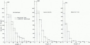
Fig. 6. Comparison of ridge distributions obtained using the Rayleigh criterion, and the 2 ft (0.61 m) criterion

Examination of Fig. 5 together with the μ_h values (number of ridges per kilometer above height h) indicates a definite pattern in the shape of the distributions. In particular, the more ridges there are the greater the mean ridge height. Examination of a number of other distributions substantiated this effect and suggests that it might be possible, to some extent, to characterize both the ridge height and spacing distribution by a single parameter. In choosing a single parameter for this purpose, common sense dictates that it should be some combination of the mean ridge height and mean ridge spacing. For this purpose, a parameter γ_h (called ridging intensity) defined by γ_h = μ_h/λ has been found to describe ridging reasonably well (Hibler and others, 1974).

An example of the efficacy of such a one parameter model is given in Fig. 7, which illustrates a plot of number of ridges per kilometer above 4 ft (1.22 m), 6 ft (1.83 m), and 8 ft (2.44 m) versus the square root of γ_h· The solid curves are constructed by an empirical procedure discussed by Hibler and others (1974). The data were taken from sixteen laser track samples each about 40 km long taken in November 1970. Fig. 8 shows the geographical location and ridging intensity of each of the 16 samples along with rough contours of the ridging intensity. A discussion of the geographical, seasonal, and annual variations of ridging intensity using 81 such samples over the period November 1970 to February 1973 is given by Hibler and others, 1974. They also discuss the sampling stability of ridging parameters and conclude that the ridging intensity γ_h is a more statistically stable parameter than the mean ridge height or the mean ridge frequency μ_h .

Fig. 7. Observed values (circles) for μ_h’, the number of ridges per kilometer above height h’ , versus γ_h; h = 4ft (l.22 m). The solid lines were constructed according to a procedure discussed by Hibler and others (1974). The observations were taken in November 1970 at locations illustrated in Figure. 8

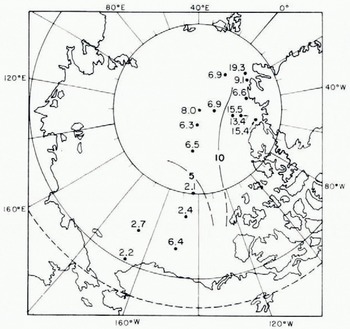
Fig. 8. Laser data sample locations and ridging intensities γ_h (h = 1.22 m) for November 1970

As a final point on ridge distribution models, we note that in some cases it may be useful simply to compile the ridge distributions empirically. The advantages of models are that they reduce the number of parameters necessary to characterize a given region and also supply an analytic functional form for other calculations such as wind form drag (see e.g. Reference AryaArya, 1973). Also, in practice, there is some sampling instability so that e.g. two adjacent 40 km segments will have different statistics. Examination of the sampling error indicates that it is commensurate with the uncertainty in prediction from the one-parameter model so that for many purposes such a model oilers adequate information to characterize ridging. In addition, it is conceptually useful to know that ridging is fairly well defined by a single parameter, since this means that if we can calculate, say, the volume of deformed ice from a sea-ice drift model, then the ridging characteristics can be estimated reasonably well.

Estimation of ridge keel depths

Besides characterizing ridge heights, laser data also provide an indirect measure of ridge keel depth distributions. For this purpose some relationship between keel depths and ridge heights is needed. Some data on this are available through measurement of individual ridges (Weeks and others, [1972]), but are too sparse to provide an adequate statistical sample. An indirect way to get keel to sail ratios is to compare height and depth percentage distributions in the same region and modify the height and depth scales until the two curves overlap. If Equation (3) is used to characterize the distribution, then it is easy to see that the probability density curves will coincide (within a constant factor) when the keel to height ratio is given by

(5)

For a rough comparison of this type, submarine data from the 1960 winter cruise of the U.S.S. Sargo (see Hibler and others, 1972) yielded λ values of about 0.0117 m^-2 near the North Pole and 0.0086 m^-2 closer to the northern Canadian Archipelago. Typical laser data from the winter of 1971 (sec Hibler and others, 1974) yielded λ values for similar regions of 0.517 m^-2 and 0.357 m^-2 which by Equation (4) gives ratios of 6.6 and 6.7. Comparison of laser data from winter 1973 would yield somewhat larger ratios. These ratios are larger than the 4.5 ratio observed by Kovacs (1972) in profiling individual ridges, but in the same range as the 7.6 ratio observed by Kan and others (1974) using sonar mapping and surface level lines. It should also be remembered here, that in data taken by Kovacs the ridge heights are generally taken to be the high points (or at least locations where the ridge is a well-defined obstacle) whereas the laser picks out whatever height it happens to go over, and there may well be a difference of several feet (a meter or two) between these measurements (Hibler and Ackley, 1973).

A graphical comparison of this type for laser and submarine sonar data has also been made in the East Greenland Sea by Reference Kozo and DiachokKozo and Diachok (1973). They found that a ratio of five gave the best agreement. These results might indicate that the East Greenland Sea and Arctic Basin ratios are different. However, both these estimated ratios may be somewhat in error. The comparison made by Kozo and Diachok for example involved only 18 km tracks with relatively shallow ridges and no more than four class intervals in the distributions. On the other hand, the comparison of λ values, although taken from larger tracks and having more class intervals, were made in different years. Also, the comparison of percentage distribution makes no use of the spacing of ridges.

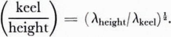
A more direct comparison which makes more complete use of the available information is to compare heights and depths where the same number of ridges per kilometer were encountered. Some data for this purpose were obtained during March 1971 near the North Pole. During this time both laser profile data (see Hibler and others, 1974) and submarine sonar data were acquired (Swithinbank, 1972; Williams and others, 1975). From these simultaneous data, we first obtained the number of ridge encounters (per km) at a given depth from the H.M.S. Dreadnought data between lat, 89° to 90° N. The laser data (using the one-parameter model with a characteristic γ_h) were used to determine heights where the same frequency of ridges was encountered. The results are shown in Figure g. The solid line represents the regression line through the data and is given by d — 6.58(h+0.17 m) (with a correlation coefficient of 0.99). Adding a small constant to the ridge height is reasonable since the three-step filtering process does not quite reduce the zero height to water level. The ratio of 6.58 is close to the ratio obtained earlier by taking λ values from different years.

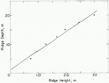
Fig. 9. Heights and depths at which the same number of ridges per kilometer were encountered. The data wen taken near the North Pole in March 1971, and consisted of submarine data reported by Williams and others (1975) and laser data reported by Hibler and others (1974)

Fig. 10. Spectral densities (part a) of moderately rough first-year ice and relatively smooth multi-year ice calculated from stereo-photogrammetric grids. Photographs showing the areas gridded are given in part b of the figure. Each spectrum represents the average of spectra along five parallel profiles 1 m apart. The average variances are 0.335 m² and 0.0343 m² for the first-year and multi-year ice spectra respectively.

Spectral roughness characteristics of sea ice

Probably the most direct and simple terrain characterization that can be derived from the laser profiles is the spectral density. Spectral densities have traditionally been used to classify terrain surfaces for purposes of vehicular ride characteristics (Reference BekkerBekker, 1969, p. 319) and they serve a similar purpose for sea ice. The spectral approach also has certain other advantages in that it appears that spectral roughness may be usable to identify ice type (Hibler and LeSchack, 1972) and to estimate wind stress over relatively unridged ice (Reference Banke and SmithBanke and Smith, 1973).

To illustrate how spectral characteristics might be used to identify ice types we illustrate, in Fig. 10, spectra of relatively flat multi-year and first-year ice. These spectra are calculated from height profiles made from stereo photos of multi-year and first-year ice as described by Mock and others (1974). As can be seen, the primary difference is that the first-year ice has somewhat more high-frequency roughness at wavelengths shorter than about 30 m. This difference suggests that an appropriate digital filter might be used to identify ice types.

Fig. 11. Spectral densities using laser profiles from three locations in Arctic Basin in November 1970. The spectra were each calculated from 4 000 data points and c. 1.4 m spacings. The ridging intensities for the tracks used were 15.4, 6.5 and 2.4 m²/km. Reference to Fig. 8 using these ridging intensities allows identification of sample location

Examination of various sea-ice spectra indicates that the spectral density has geographical variations similar to those of ridging intensity. Some typical spectral densities shown in Fig. 1 1 illustrate this effect. The spectral densities shown in this figure are taken from similar geographical regions as the ridge distributions in Fig. 5. As can be seen, the slope of the double logarithmic spectral plots generally decrease as one proceeds from the heavily ridged region near the northern Canadian Archipelago to the more lightly ridged Beaufort Sea region. The slope of the double logarithmic plots lie between — 2 and —3. The —3 slope is especially interesting, since, as noted by Reference NyeNye (1973), such a slope is indicative of a terrain which “looks the same” at all scales.

To quantify the relationship between the spectral roughness of the sea ice and its ridging intensity it is useful to correlate the r.m.s. roughness parameter ζ_z , with γ_h , where ζ_z is defined by

(6)

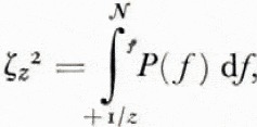
N_f being the Nyquist frequency in cycles per meter and P(f) the power spectrum. ζ_z thus represents the r.m.s. surface roughness at wavelengths shorter than z. To carry out the calculation of ζ_z , we used the first 4 000 data points from the 16 November 1970 samples. The lag product method with 200 lags and a Hamming spectral window was used to calculate P(f)> and ζ_z was calculated for z = 13 m and 200 m. Some of the results of these calculations are shown in Table I and Fig. 12.

Table I. Correlation co-efficient between spectral and ridge parameters

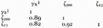
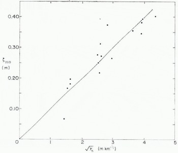
Fig. 12. ζ₂₀₀, r.m.s. surface roughness for wavelengths less than 200 m, versus γ_h ½; h = 4 ft (1.22 m). The sample location (and γ_h values) are identified in Fig. 8.

Fig. 12 illustrates the high correlation between ζ₂₀₀ and the square root of the ridging intensity. The least-squares line has the form ζ₂₀₀ = mγ_h ½ with m = 0.0989 km ½. Although not illustrated, a plot of ζ₁₃ versus λ_h ½ shows a similar trend to that in Fig. 12 with an m value of 0.0319 km½. The implication of these results is that to a limited extent ridging intensity γ_h can be used to estimate spectral roughness as well as ridging.

Spectral characteristics of tundra

As discussed under the description of the laser profile data, when information on a given terrain in a frequency range 300 m to 2 m is desired, laser profilometry is useful. Tundra is an example of such a terrain, since it is commonly characterized by polygonal ground varying over lengths of several meters. Typical spectral densities of tundra before and after a snowfall are shown in Fig. 13. The profiles for these spectra were made by hand at 0.5 m intervals. Examination of a number of other profiles besides this one (private communication from S. Mock) indicates that the spectral density is quite well described by P(f) = Ωfⁿ with n in the range —1.4 to —2.19 and log Ω varying from o to 0.64 (SI units used).

Work is underway to determine if this functional form can be extended to higher frequencies. If so, then laser profilometry would indirectly supply a measure of higher-frequency roughness characteristics, in that the spectral “window” from f₁ to f₂ could be used to estimate the parameters Ω and n.

Fig. 13. Tundra spectra of summer and winter profiles (taken at the same location) and snow depth. Each profile consisted of 260 points at 0.5 m spacings measured by spirit level before and after snowfall. The profile was located near Pt. Barrow, Alaska

Another dividend here is the similarity of summer-profile spectra and the snow-depth spectra. What has happened, of course, is that the snow has generally filled in the rapid terrain variations and thus the snow-depth spectrum is similar to the terrain profile spectrum. Coherence studies verify this and show the snow depth to be highly coherent with a phase shift of 18o° as would be expected. This coherence does drop off” at low frequencies however. Comparison of profiles before and after snowfall would allow some determination of this low-frequency cut-off and allow a statistical estimation of the variations in snow depth. Such information could be useful for water run-off studies, since a region with greater high-frequency roughness might trap more snow.