


Introduction
The sea ice/snow system plays a major role as an atmosphere/ocean interface and is an optical medium controlling light availability for sympagic and pelagic ecosystems including sea-ice algae (e.g. Gosselin and others, Reference Gosselin, Legendre, Therriault, Demers and Rochet1986; Mundy and others, Reference Mundy, Ehn, Barber and Michel2007; Campbell and others, Reference Campbell, Mundy, Barber and Gosselin2015; Lange and others, Reference Lange2019). Bio-optical observations of hyperspectral light distributions under sea ice have been studied and have yielded new insights into noninvasive estimates of sea-ice algal biomass in Antarctica (Melbourne-Thomas and others, Reference Melbourne-Thomas2015, Reference Melbourne-Thomas2016; Meiners and others, Reference Meiners2017; Wongpan and others, Reference Wongpan2018), in the Arctic (Perovich and others, Reference Perovich, Cota, Maykut and Grenfell1993; Mundy and others, Reference Mundy, Ehn, Barber and Michel2007; Campbell and others, Reference Campbell, Mundy, Barber and Gosselin2015; Lange and others, Reference Lange, Katlein, Nicolaus, Peeken and Flores2016)d in Greenland (Lund-Hansen and others, Reference Lund-Hansen2018). However, sea-ice bio-optical studies remain scarce in nonpolar sea ice, for example, the Baltic Sea (Granskog and others, Reference Granskog2004; Uusikivi and others, Reference Uusikivi, Vähätalo, Granskog and Sommaruga2010) or Saroma-ko Lagoon (Robineau and others, Reference Robineau, Legendre, Kishino and Kudoh1997).
Saroma-ko Lagoon is located on the Okhotsk Sea coast of Hokkaido, Japan and is one of the lowest-latitude areas where sea ice forms (Liu and others, Reference Liu, Saitoh, Maekawa, Mochizuki and Tian2018). In winter, sea ice grows fastened to the coastline. Seawater from the Sea of Okhotsk enters the lagoon via two inlets (e.g. Nomura and others, Reference Nomura2009, Reference Nomura, McMinn, Hattori, Aoki and Fukuchi2011). The lagoon has been investigated spatially at kilometre scales for its sea-ice algal biomass distribution (Robineau and others, Reference Robineau, Legendre, Kishino and Kudoh1997) and temporally at the decadal scale with regard to its ice-cover variability (Liu and others, Reference Liu, Saitoh, Maekawa, Mochizuki and Tian2018), and has been used for sea-ice research education, process studies, protocol testing and inter-comparison of sea-ice bio-optical sensors (Roukaerts and others, Reference Roukaerts2018; Nomura and others, Reference Nomura2020; Toyota and others, Reference Toyota, Ono, Tanikawa, Wongpan and Nomura2020).
Horizontal heterogeneity of algal distribution in Saroma-ko Lagoon sea ice with a uniform snow cover has been previously demonstrated by Robineau and others (Reference Robineau, Legendre, Kishino and Kudoh1997). These authors used ice-coring methods (bottom 0.03 m) along a 4 km transect and revealed the patchiness of the ice-algae distribution at scales of 70, 100 and 500 m. The study showed that ice-bottom salinity explained 68% of the variability of the vertically integrated chlorophyll a (Chl. a) (Robineau and others, Reference Robineau, Legendre, Kishino and Kudoh1997). The study also suggested that the horizontal heterogeneity of sea-ice algal biomass of the lagoon could be neglected at scales <20 m and that salinity of the water column could potentially be a physical control of sea-ice algal biomass as previously shown for Hudson Bay sea ice (Canadian Arctic) (Legendre and others, Reference Legendre, Aota, Shirasawa, Martineau and Ishikawa1991), where the crystallographic structure of sea ice also plays an important role in sea-ice algal distribution.
There are growing needs to upscale sea-ice algal biomass estimations for biogeochemical and primary production model evaluation (Nishi and Tabeta, Reference Nishi and Tabeta2005, Cimoli and others, Reference Cimoli, Meiners, Lucieer and Lucieer2019) and to establish baselines from which to monitor Saroma-ko Lagoon decadal scale changes (Liu and others, Reference Liu, Saitoh, Maekawa, Mochizuki and Tian2018). To increase the coverage and upscale observations, development of bio-optical relationships is a way forward from classical sea-ice coring methods for using and validating data from under-ice remote-sensing platforms such as unmanned underwater vehicles (e.g. review by Cimoli and others, Reference Cimoli, Meiners, Lund-Hansen and Lucieer2017). Underwater vehicles have been used to estimate ice algal biomass at 100–1000 m scales (Lange and others, Reference Lange, Katlein, Nicolaus, Peeken and Flores2016; Lange and others, Reference Lange2017; Meiners and others, Reference Meiners2017; Lund-Hansen and others, Reference Lund-Hansen2018; Forrest and others, Reference Forrest2019). Melbourne-Thomas and others (Reference Melbourne-Thomas2015) compared several approaches to estimate Antarctic sea-ice algal biomass from under-ice optical measurements at regional scales including Empirical Orthogonal Functions and Normalised Difference Index (NDI) and concluded that NDI explained the highest percentage of variance. Cimoli and others (Reference Cimoli, Meiners, Lucieer and Lucieer2019) provided a novel solution using an under-ice hyperspectral and RGB imaging system to explore the algal biomass distribution at the sub-metre scale. These authors also introduced an index, previously used in terrestrial vegetation mapping (Malenovsky and others, Reference Malenovsky2006), to sea-ice algal research which uses the red (650–700 nm) bandwidth of under-ice irradiance spectra to estimate ice algal biomass.
This study is the first attempt to develop an NDI-ice algal biomass relationship for first-year land-fast sea ice in Saroma-ko Lagoon. Relationships between sea-ice physico-biogeochemical parameters and ice algal biomass were also investigated. Furthermore, we combined sea-ice algal biomass from coring measurements and NDI-approximations to explore the spatial heterogeneity of Saroma-ko Lagoon sea-ice algal biomass using a geostatistical approach.
Data and methods
Study area
Our observations were part of the ‘Saroma-ko Lagoon Observations for sea ice Physico-chemistry and Ecosystems 2019’ program (SLOPE2019; Nomura and others, Reference Nomura2020). The mean depth of the lagoon is 14.5 m and its surface area is ~150 km2. Figure 1 shows the locations of 27 paired in situ sea-ice optical and biological measurements along three transect lines (256 m) across multiple scales covering an area of over 250 m × 250 m, carried out from 22 to 28 February 2019. Sampling location C2 was located at N44°7′91′′E143°57′238′′, ~2 km off the eastern shore of Saroma-ko Lagoon (Fig. 1). This location was centred within a 4 km quadrant chosen to avoid sharp meridional salinity gradients caused by the Saromabetsu river inflow and the lagoon's connection to the Sea of Okhotsk (Robineau and others, Reference Robineau, Legendre, Kishino and Kudoh1997).
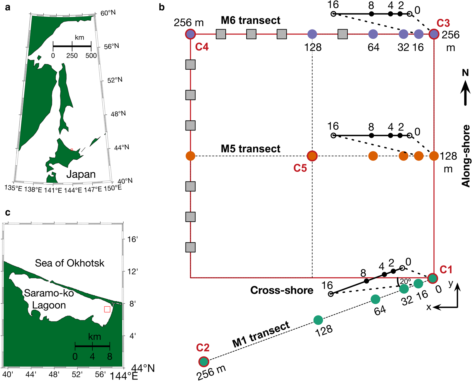
Fig. 1. Study area. (a) Map of Sea of Okhotsk and Hokkaido island, Japan and (b) Saroma-ko Lagoon, Hokkaido, Japan. (c) The study grid was connected with C2 (the main station of SLOPE2019 (Nomura and others, Reference Nomura2020)) by the M1 transect. Circles denote sites with paired measurements of under-ice transmittance and Chl. a (from ice cores) and grey squares represent sites at which only under-ice transmittance was measured. Note that there are ice stations at 2, 4 and 8 m between 0 and 16 m for all three transects.
Spatial variability: integrated sea-ice bio-optical sampling
In this section, the protocol of sampling sea-ice cores at each grid site is described. We conducted sampling along three east-to-west transects: M1, M5 and M6. Each transect was composed of nine stations: 0, 2, 4, 8, 16, 32, 64, 128 and 256 m (Fig. 1).
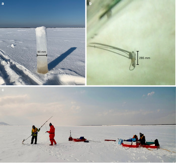
At each station, the first sea-ice core (Core A) was collected with an ice corer (Mark II coring system, Kovacs Enterprises, Inc., Oregon, USA) with an inner and outer diameter of 90 and 110 mm, respectively. The ice-core length was measured using a ruler. Temperatures were measured within 5 minutes of coring as in Pringle and Ingham (Reference Pringle, Ingham, Eicken, Gradinger, Salganek, Shirasawa, Perovich and Leppäranta2009) by inserting a needle-type temperature sensor (Testo 110 NTC, Brandt Instruments, Inc., Los Angeles, USA) into small holes (~20 mm deep) drilled into the core at 100 mm resolution, starting 20 mm from the bottom, with a final measurement 20 mm from the top (Nomura and others, Reference Nomura2009). Extracted ice cores were placed in polythene bags, labelled and stored horizontally in a cooler box along with ice packs to minimise brine drainage and to maintain low temperatures. Thereafter, the ice cores were stored frozen locally in a chest freezer and transported to the Institute of Low Temperature Science, Hokkaido University and stored at −15°C for the sea-ice structure and texture analysis.
Two TriOS RAMSES ACC UV/VIS hyperspectral radiometers (TriOS GmbH, Rastede, Germany) were used for a spatial survey of the above-ice and under-ice hyperspectral light transmission (Fig. 2b). The RAMSES have a resolution of 3.3 nm and cover the wavelength range of 280–720 nm. For the optical set-up, the first TriOS sensor was mounted onto a tripod to observe the incident hyperspectral irradiance. To avoid light pollution from the Core A hole (110 mm in diameter), a retractable L-arm was used to deploy the second sensor (Figs 2b and c) to measure the transmitted hyperspectral irradiance 1.3 m away from the access hole and 0.075 m under the ice/ocean interface (to minimise light absorption by the water column). At least three replicate measurements were taken concurrently with the two sensors. The measured spectra were interpolated to 1 nm resolution and the hyperspectral transmittance in the 400–700 nm hyperspectral band (photosynthetically active radiation (PAR)) was calculated as the ratio of hyperspectral transmitted irradiance to incident hyperspectral irradiance.
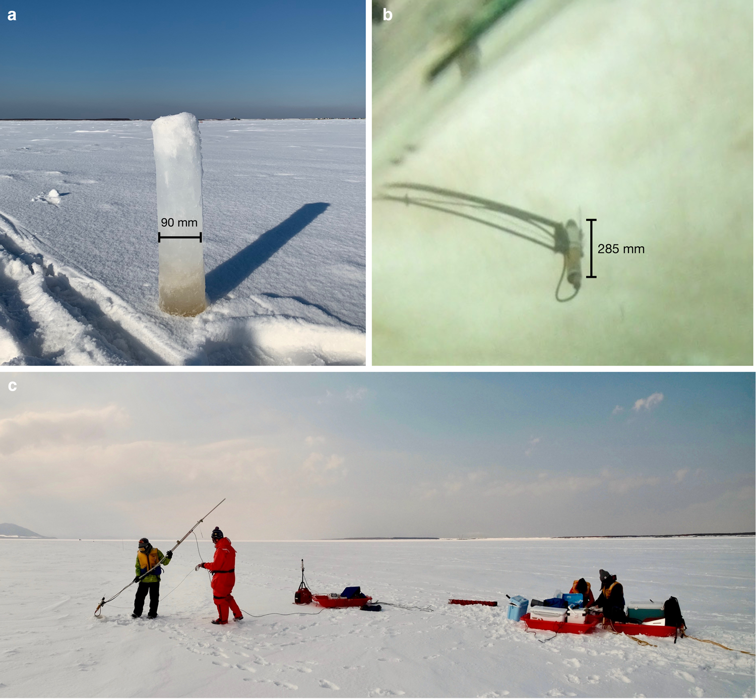
Fig. 2. Integrated physico-biogeochemical observations at Saroma-ko Lagoon. (a) A typical 90 mm diameter sea-ice core from Saroma-ko Lagoon. (b) Under-ice irradiance sensor in operation. This sensor was measuring the light transmitted through snow, sea ice and absorbed by sea-ice algae. (c) Deployment of the irradiance sensor through the borehole (as in (b)) with concomitant measurement of a temperature profile by other team members. Pictures (b) and (c) were taken from Nomura and others (Reference Nomura2020), with permission from the Bulletin of Glaciological Research, the Japanese Society of Snow and Ice.
Following the optical measurements, five replicate snow-thickness measurements were made above the under-ice sensor position (1.3 m away from Core A pointing towards the sun) using a ruler. Snow was sampled with a plastic shovel and stored in a press-seal bag. After removing snow, the second sea-ice core (Core B) was collected at the sensor position. Next, the core length and the freeboard were recorded. Core B was then cut into three vertical sections: the bottom 100 mm and two remaining sections of equal length. These were stored in press-seal bags and kept horizontally in a cooler box for transport back to a shore-based laboratory in Napal Kitami near the sampling site. The samples were melted in the dark at room temperature without adding filtered seawater (Rintala and others, Reference Rintala2014; Roukaerts and others, Reference Roukaerts2018). The melting process was checked regularly and towards the end, samples were swirled until the last pieces of ice had melted before immediate processing.
Sea-ice bulk salinity was measured with a conductivity sensor (Cond 315i, WTW GmbH, Germany) and aliquots were taken for determination of nutrient concentrations (NO2 + NO3, PO4, and SiO2) with a QuAAtro 2-HR system (BL-Tec, Osaka, Japan; Seal Analytical, Southampton, UK). Next, 100 mL subsamples were filtered onto 25 mm diameter glass fibre (Whatman GF/F filters) for Chl. a analysis. After extraction using N, N-dimethylformamide (DMF) for 24 hours (Suzuki and Ishimaru, Reference Suzuki and Ishimaru1990), the Chl. a concentrations of samples were determined fluorometrically (Welschmeyer, Reference Welschmeyer1994) using a fluorometer (10 AU, Turner Designs, San Jose, USA) calibrated with pure Chl. a (FUJIFILM Wako Pure Chemical Corporation). From the filtrate, oxygen isotopic ratios (δ 18O) were determined with a Picarro L2120-i (Picarro Inc., Santa Clara, USA). Lugol's solution was added to the remaining unfiltered sample for taxonomic analyses. A microscope (IMT-2, Olympus, Tokyo, Japan) with 40 × objective and 10 × oculars was used for cell counts. Identification of ice algae followed Tomas (Reference Tomas1997), and Scott and Marchant (Reference Scott and Marchant2005). Following standard protocols (Langway, Reference Langway1958), the ice cores from C1, C2, C3, C4 and C5 were processed in a cold laboratory (−15°C) at the Institute of Low Temperature Science, Hokkaido University to study the spatial variability of sea-ice structure. Thick sections (~5 mm) were cut using a bandsaw to examine brine pockets and air bubbles. A microtome was used to reduce thick sections to thin sections (<1 mm) to study the sea-ice texture in detail using cross-polarising filters to identify whether samples consisted of granular or columnar ice.
To monitor physico/biogeochemical changes at the site during the observation period, a temporal variability study was conducted at site C2 on 23 (16:00 LT), 25 (15:45 LT) and 27 February 2019 (15:49 LT). A sampling protocol similar to that for the spatial variability study was applied but with the higher vertical resolution (every 0.05–0.10 m). In addition, under-ice water samples were collected at least 15 minutes after the core extraction (Nomura and others, Reference Nomura, McMinn, Hattori, Aoki and Fukuchi2011). Seawater samples were collected through the borehole using a 500 mL Teflon water sampler (GL Science Inc., Tokyo, Japan) at 1 and 5 m depth below the bottom of the sea ice. Salinity, nutrients and δ 18O were measured in the same manner as sea-ice meltwater for the spatial variability sites.
Normalised difference index
Hyperspectral transmittance (T E) is defined as the ratio of under-ice transmitted irradiance (E T) to incident irradiance (E S):

where λ is wavelength in the photosynthetically active radiation (PAR) range between 400 and 700 nm (Fig. 3).
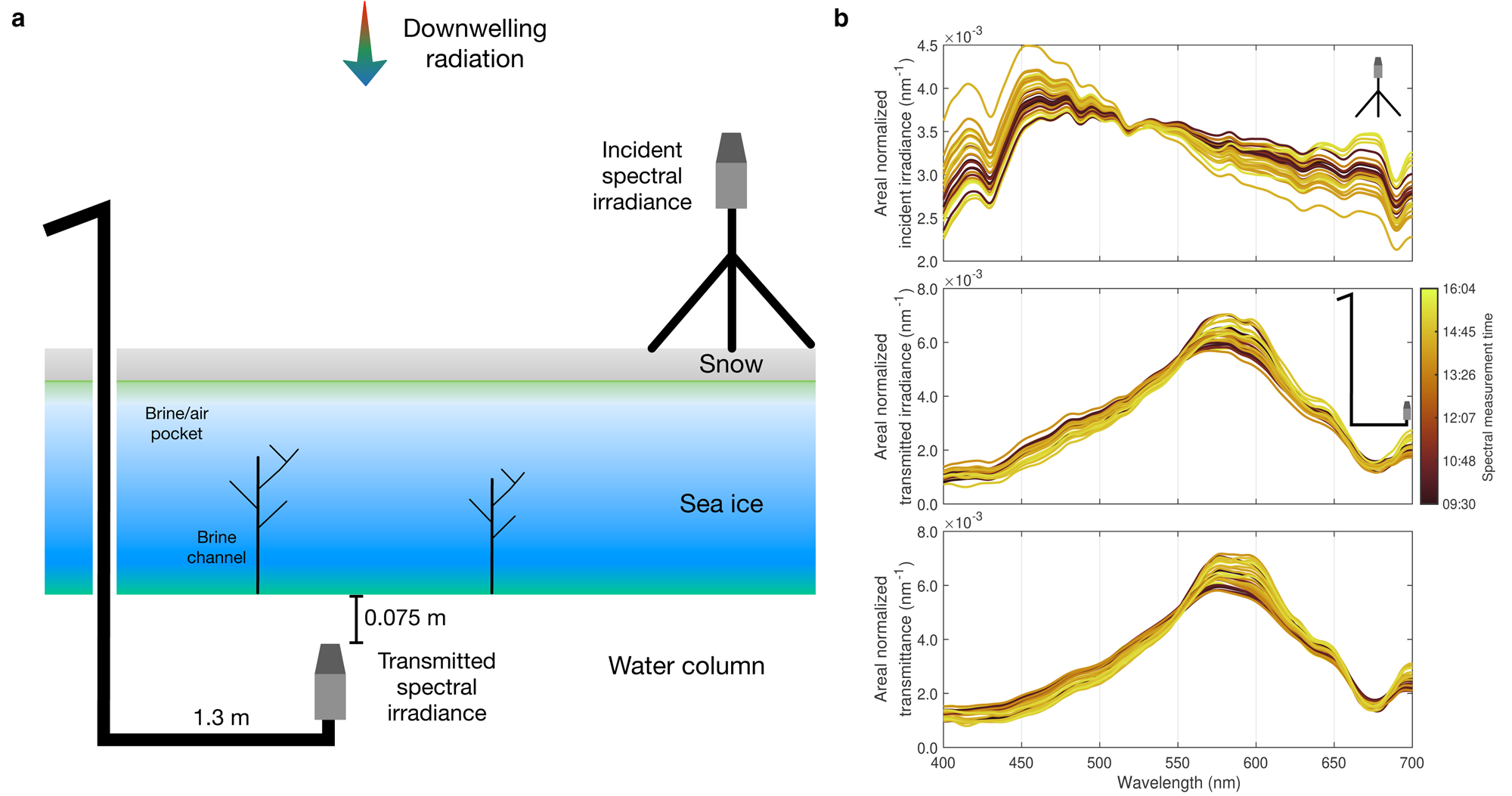
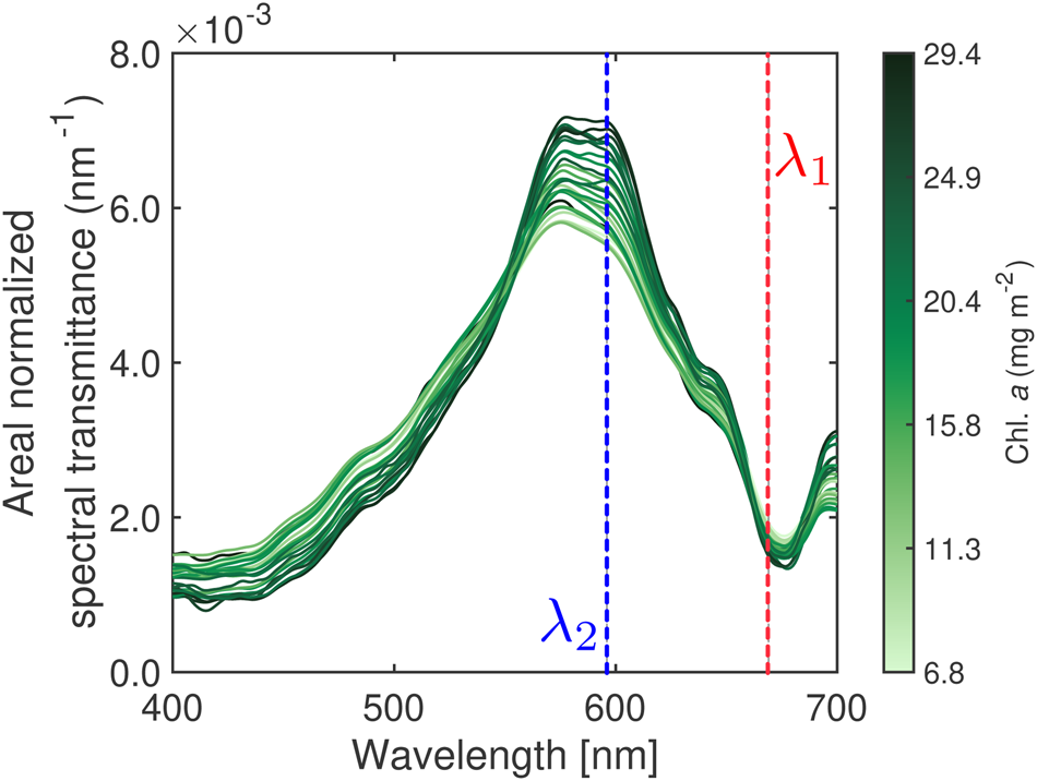
Fig. 3. Hyperspectral transmittance. (a) Schematic shows the optical set-up to retrieve hyperspectral transmittance. (b) Synchronous measurement of incident and transmitted hyperspectral irradiances and hyperspectral transmittances at 27 stations (see Fig. 1) normalised by areas under the curve. Note that the spectrum at Station C2 was removed from the analysis due to the late time of sampling (16:05 LT on 23 February 2019, Fig. S1).
In order to explore the correlation between the hyperspectral transmittance and Chl. a, the dimension of hyperspectral transmittance for each station was reduced to a single wavelength pair using the NDI formula. NDI is defined here as:

With all possible combinations of λ 1 and λ 2 using log10(Chl.a[mg m−2]) as a response and NDI(λ 1, λ 2) as a predictor, we applied linear regression analysis and searched for the maximum coefficient of determination (R 2) of the form:

where a is a slope and b is an intercept. Note that log-transformed Chl. a data were used following Melbourne-Thomas and others (Reference Melbourne-Thomas2015), Lange and others (Reference Lange, Katlein, Nicolaus, Peeken and Flores2016) and Wongpan and others (Reference Wongpan2018). To select the best pair of λ 1 and λ 2 we constructed an R 2 correlation-surface and searched for the maximum R 2 following the approach of Mundy and others (Reference Mundy, Ehn, Barber and Michel2007) and Wongpan and others (Reference Wongpan2018). We limited our search to areas within the broad and narrow Chl. a absorption bands centred around 440 and 670 nm, respectively, as suggested by Lange and others (Reference Lange, Katlein, Nicolaus, Peeken and Flores2016). The analysis was performed with MATLAB R2019a (The MathWorks Inc.) and used the cmocean colorbar toolbox (Thyng and others, Reference Thyng, Greene, Hetland, Zimmerle and DiMarco2016). Note that we also examined the NDI-relationship using transmitted irradiance instead of transmittance (Fig. S2). The resultant irradiance-based relationship was not as strong as that of the transmittance-based NDI (Eqn 2) and thus, was not used. Note also that PAR transmittance correlates with Chl. a (Fig. S3).
Spatial autocorrelation analyses of Chl. a and sea-ice properties
To quantify the horizontal patchiness of Chl. a, ice thickness, snow depth and freeboard, we used a correlogram, for example, a plot of Moran's I estimates (Moran, Reference Moran1950, Legendre and Fortin, Reference Legendre and Fortin1989; Legendre and Legendre, Reference Legendre, Legendre, Legendre and Legendre2012) as a function of the distance between sites (distance class). Following Lange and others (Reference Lange2017) and Fletcher and Fortin (Reference Fletcher and Fortin2018), we used the R (R Core Team, 2020) pgirmess package (Giraudoux, Reference Giraudoux2018) using the correlog function. We truncated the utilised maximum distance to be 2/3 of the actual maximum distance (Fletcher and Fortin, Reference Fletcher and Fortin2018). We applied a Bonferroni adjustment correction (p < 0.05/n, where n is the number of distance class) to test for the global significance with 10 distance classes (p < 0.005 at 0.05 significance level, two-sided). The first x-intercept of the global significance correlograms was used to estimate the patch size of Chl. a, ice thickness, snow depth and freeboard and to investigate the physical drivers of the Chl. a spatial distribution (Lange and others, Reference Lange2017 and references therein).
Results and discussion
We analysed physical properties of snow and ice to support the 27 paired in situ optical and biological measurements collected along four transect lines covering an area of over 250 m × 250 m (Fig. 1).
Mean snow depth and ice thickness in the study areas were 0.08 ± 0.01 m (N = 135) and 0.48 ± 0.03 m (N = 27), respectively. The water depth at the C2 station was ~6 m. Variability of snow depth and ice thickness was low and ranged between 0.06–0.10 m and 0.41–0.56 m, respectively. These data are comparable to those found by Robineau and others (Reference Robineau, Legendre, Kishino and Kudoh1997) reporting snow depths and ice thicknesses of 0.11 ± 0.03 m and 0.41 ± 0.08 m, respectively. Sea-ice freeboard was always positive and ranged from 0.03 ± 0.01 m (N = 27) due to the thin snow cover. Snow depth was inversely correlated with ice thickness and bottom 0.1 m brine volume fraction (Fig. 4).
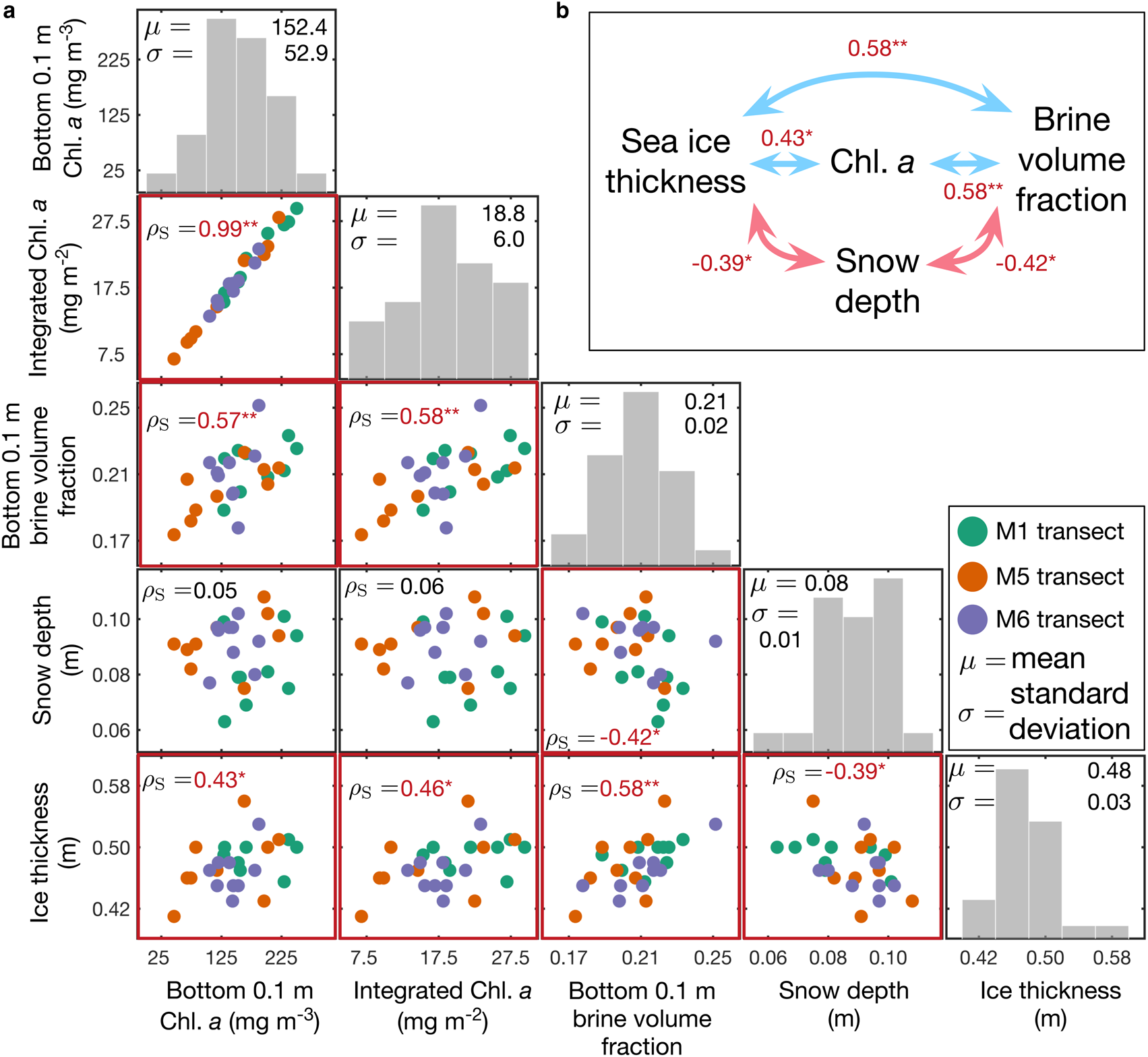
Fig. 4. Frequency distributions of and relationships between, sea-ice physical and biogeochemical parameters. (a) Spearman's rank correlation coefficients (red) for relationships of selected physical and biogeochemical parameters. Note that * denotes 0.01 < p < 0.05 and ** denotes p < 0.01. Otherwise nonsignificant or p > 0.05. (b) Summary of significant correlations among physical and biogeochemical parameters. Note that bin widths of histograms are 50 mg m−3, 5 mg m−2, 0.02, 0.01 m and 0.04 m from left to right.
The mean concentrations of Chl. a in the bottom 0.1 m of the sea-ice cores ranged between 46.1 and 250.4 mg m−3 with a mean of 152.4 ± 53.0 mg m−3 (N = 27, Fig. 4). Note that Chl. a in μg L−1 in all sections including snow were integrated over the entire ice thickness and expressed as integrated Chl. a (mg m−2). The mean depth-integrated Chl. a concentration was 18.8 ± 6.0 mg m−2 with a range of 6.8–29.4 mg m−2. These values are similar to values (28.2 ± 22.5 mg m−2) reported by Robineau and others (Reference Robineau, Legendre, Kishino and Kudoh1997). However, integrated Chl. a values from Saroma-ko Lagoon show high interannual variation, for example, 2.0–9.0 mg m−2 in 2008 and 0.3–10.6 mg m−2 in 2009 (Granskog and others, Reference Granskog2015) with maximum mean values of 272.8 ± 20.2 mg m−2 (McMinn and Hattori, Reference McMinn and Hattori2006). We speculate that this is due to the multidecadal variability in sea-ice cover in Saroma-ko Lagoon (Liu and others, Reference Liu, Saitoh, Maekawa, Mochizuki and Tian2018). Liu and others (Reference Liu, Saitoh, Maekawa, Mochizuki and Tian2018) illustrated that the ice coverage and water temperature during winter, both affected by local climate, are key environmental factors in the algal bloom development and variation in Saroma-ko Lagoon. Long-term monitoring of spatial and temporal variability of Saroma-ko sea-ice algal biomass is needed to identify key physical drivers and assess consequences of the environmental change on sympagic and pelagic ecosystems in the lagoon (Liu and others, Reference Liu, Saitoh, Maekawa, Mochizuki and Tian2018).
Relationships between physical and biological sea-ice parameters were explored using Spearman's rank correlation coefficients (ρ S). The Chl. a concentrations in the bottom 0.1 m of the sea-ice core were highly correlated with the entire ice core integrated Chl. a values (ρ s = 0.99, p < 0.01) because most of the sea-ice algal biomass was concentrated close to the ice/water interface. The correlation between snow depth and Chl. a in the bottom 0.1 m of the sea ice was not significant (ρ s = 0.05, p = 0.79). The correlation between the ice-bottom salinity and integrated Chl. a was also not significant (p > 0.05), which supports our site selection that aimed to avoid the influence of a salinity gradient (Robineau and others, Reference Robineau, Legendre, Kishino and Kudoh1997). However, there was a strong positive correlation between the brine volume fraction and the Chl. a in the bottom 0.1 m of the sea-ice cores (ρ s = 0.57, p = 0.02; see Fig. 4).
We found a positive correlation between ice thickness and algal biomass distribution (ρ s = 0.46, p = 0.02). Snow depth correlated with ice thickness (ρ s = − 0.39, p = 0.04) but did not correlate directly with algal biomass (ρ s = 0.06, p = 0.78) similar to results reported by Robineau and others (Reference Robineau, Legendre, Kishino and Kudoh1997). Our findings (Fig. 4b) demonstrate the complexity of the interrelationships among sea-ice physical parameters and their use as predictors for the sea-ice algal biomass (Lange and others, Reference Lange2017; Meiners and others, Reference Meiners2017).
The variability in sea-ice texture, ice thickness and sea-ice algal biomass at the four corners (C1–C4) and the centre of the grid site (C5) is illustrated in Figure S4. In particular, C2 and C3 have the same ice thickness (~0.45 m) but the Chl. a concentrations in the bottom 0.1 m of the sea-ice cores vary by 58.4%: with 229.3 mg m−3 for C2 and 144.8 mg m−3 for C3. The columnar ice proportion of individual ice cores was relatively small and variable and could have played a partial role in the spatial variability of ice algal biomass in Saroma-ko Lagoon, similar to results from southeastern Hudson Bay (Legendre and others, Reference Legendre, Aota, Shirasawa, Martineau and Ishikawa1991). Sea-ice structure archives the thermo-halodynamic and meteorological forcing history of its growth and influences biogeochemical interactions and ice algal growth due to different permeability thresholds and interior surface area (Golden and others, Reference Golden, Ackley and Lytle1998, Krembs and others, Reference Krembs, Gradinger and Spindler2000).
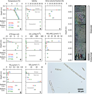
The temporal variability study at C2 over the period of 5 days was compiled in Nomura and others (Reference Nomura2020) and Toyota and others (Reference Toyota, Ono, Tanikawa, Wongpan and Nomura2020) and is only briefly summarised here. Figure 5 shows the vertical profiles of temperature, salinity, brine volume fraction, oxygen isotopic ratio and nutrients (NO2 + NO3, PO4 and SiO2) and Chl. a concentrations within snow, sea ice and the water column (1 and 5 m depth below the bottom of the sea ice) at site C2. Vertical temperature profiles in sea ice were remarkably stable through the observation period (Fig. 5a). In contrast, temperature profiles in the snow were more variable (Fig. 5a). This is because the specific heat of saline ice is much higher than that of snow, buffering temperature changes in sea ice (e.g. Schwerdtfeger, Reference Schwerdtfecer1963). The variability in snow temperature reflected changes in the air temperatures (Figure S1). The salinity profiles within the sea ice were generally C-shaped (Fig. 5b) and the snow/ice interface showed high salinities (S > 17). Vertical profiles of δ 18O in sea ice indicated that the top of sea ice consisted of snow ice with low δ 18O (Fig. 5d).

Fig. 5. Short-term change in physical and biogeochemical parameters from site C2. Vertical profiles of (a) ice temperature, (b) salinity, (c) brine volume fraction (d) δ 18O, (e) Chl. a, (f) NO2 + NO3, (g) PO4, (h) SiO2, (i) ice texture from thin section sampled on 25 February 2019 (Picture adapted from Nomura and others, Reference Nomura2020) and (j) a micrograph of the ice algal assemblage from the bottom 0.1 m of the sea-ice core. Pictures (i) and (j) were taken from Nomura and others (Reference Nomura2020), with permission from the Bulletin of Glaciological Research, the Japanese Society of Snow and Ice.
Sea-ice algal abundance was dominated by diatoms (98%) with the remaining 2% composed of cryptophytes and dinoflagellates (Fig. 5j). Similar to the spatial survey, Chl. a concentrations at the temporal site were high at the bottom of the sea ice (>166 mg m−3, Fig. 5f). Compared to the literature concerning the same site, these concentrations were high, with Nomura and others (Reference Nomura, McMinn, Hattori, Aoki and Fukuchi2011) reporting a Chl. a concentration of 55.4 mg m−3 at the bottom of sea ice with a snow depth of 0.14 ± 0.03 m (N = 8) in 2008. The high concentrations are likely attributed to the thin snow layer allowing higher light transmission during sampling for this study. Vertical profiles of nutrients in sea ice indicated high concentrations of NO2 + NO3 in the upper part of the sea ice (Fig. 5f) that can be attributed to atmospheric supply via snowfall and incorporation into the sea ice by snow-ice formation (Nomura and others, Reference Nomura, McMinn, Hattori, Aoki and Fukuchi2011). On the other hand, concentrations of PO4 and SiO2 in snow and the upper part of the sea ice were low (Figs 5g and h) indicating that snowfall and snow-ice formation made only a minor contribution to these nutrient pools. Concentrations of SiO2 in the bottom of the ice were higher than in the under-ice water suggesting the dissolution of biogenic opal from sea-ice diatoms (Fig. 5g). Figure 5i, showing the vertical thin-section photographs of the sea-ice core at site C2 on 25 February 2019, indicates that most of the ice was dominated by granular ice consisting of snow-ice and frazil ice (89% of the ice thickness in the upper parts of the ice core), with columnar ice making up the remaining 11% in the lower parts of the ice core.
NDI algorithm for Saroma-ko Lagoon
Following Wongpan and others (Reference Wongpan2018), we inspected the relationship between sea-ice hyperspectral transmittance and integrated Chl. a (Fig. 6). Our findings confirm the association between the variation of the hyperspectral transmittance shape (high to low) and Chl. a variability (light to dark green), where low transmittance (high Chl. a absorption) occurs near 440 nm and 670 nm, resembling the Chl. a specific absorption maxima.
Applying the NDI approach (Mundy and others, Reference Mundy, Ehn, Barber and Michel2007; Wongpan and others, Reference Wongpan2018), we observed the empirical relationship:

where −2.95 is the slope and −0.44 is the intercept (Fig. 7b) with the highest R 2 = 0.63 (Fig. 7a), when one of the wavelengths is limited to the 665–675 nm wavelength range (Fig. 7a).
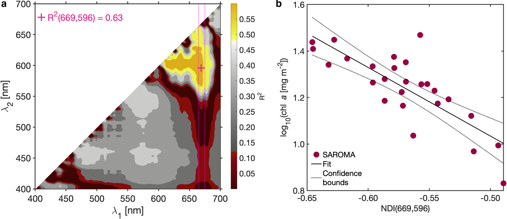
Fig. 7. The NDI algorithm for Saroma-ko Lagoon. (a) The coefficient of determination (R 2) surface constructed from all possible wavelength pairs in Eqn 3. (b) An example (and the best pair) of the linear fit used to construct the NDI relationship and represented as a pink cross in (a).
Our best wavelength pair (669, 596) is in the same wavelength range and has similar performance compared to findings by Lange and others (Reference Lange, Katlein, Nicolaus, Peeken and Flores2016) reporting that the wavelength pair (684, 678) described 70% of sea-ice algal biomass variability in the Central Arctic Ocean. Note that the study of Lange and others (Reference Lange, Katlein, Nicolaus, Peeken and Flores2016) was conducted in a late summer and there was nearly no snow. In Lange and others (Reference Lange, Katlein, Nicolaus, Peeken and Flores2016), snow depth variation correlated poorly with the variability of Chl. a (ρ s = 0.05, p > 0.05) which is corresponding to our finding (ρ s = 0.06, p = 0.78). However, in our study, the best performing wavelength pair is closer to the second narrow absorption peak of Chl. a which is not the first broader peak near 440 nm reported by Mundy and others (Reference Mundy, Ehn, Barber and Michel2007) and Campbell and others (Reference Campbell, Mundy, Barber and Gosselin2014) who suggested the best wavelength pairs of (485, 472) and (490, 478), respectively.
We suggest that specific NDI wavelength pairs near the 670 nm absorption band of Chl. a is applicable under snow-free/high-biomass sea-ice conditions (e.g., Cimoli and others, Reference Cimoli, Meiners, Lucieer and Lucieer2019), where a large part of downwelling blue light is absorbed by the primary absorption peak of Chl. a (due to high biomass) but where there is sufficient light in the red part of the spectrum to allow for an adequate NDI signal. Environmental conditions that favour an NDI wavelength pair in the orange/red part of the spectrum for Saroma-ko Lagoon, which has some snow and medium biomass, include the high coloured dissolved organic matter (CDOM) concentrations in the lagoon (Granskog and others, Reference Granskog2015) absorbing light at lower wavelengths (blue) and the overall high light transmittance (including red light) due to the relatively thin ice cover (~0.5 m).
We evaluated our NDI algorithm for Saroma-ko Lagoon with a hyperspectral transmittance survey of 10 sites at locations illustrated with grey squares in Figure 1b on 28 February 2019 at 32 m resolution. In this case, only Core A was drilled as an access hole for the L-arm. Estimated values of sea-ice algal biomass for these 10 sites were plotted and compared to values calculated using an NDI-relationship developed for Arctic fast ice and under-ice irradiance spectra (Mundy and others (Reference Mundy, Ehn, Barber and Michel2007), Fig. 8). Both relationships consistently display the same trend of spatial variation. Chl. a from our relationship provides values within the range of the coring method (N = 27) which was 18.8 ± 6.0 mg m−2, while the estimate based on Mundy and others (Reference Mundy, Ehn, Barber and Michel2007) was 93.5 ± 8.6 mg m−2. We also compared our relationship with the Central Arctic NDI relationship (Lange and others, Reference Lange, Katlein, Nicolaus, Peeken and Flores2016, Fig. 8) which resulted in a different trend compared to the Saroma-ko-specific and the Mundy and others (Reference Mundy, Ehn, Barber and Michel2007) relationships. The differences among the empirical relationships are likely a result of differences in sea-ice thickness, latitude and solar inclination, ice algal community type and pigment composition, CDOM and snow depth between the study areas. Furthermore, the study by Lange and others (Reference Lange, Katlein, Nicolaus, Peeken and Flores2016) was conducted in summer and sampled a wide range of ice types of different thickness and including bare ice and ice floes covered by melt ponds.
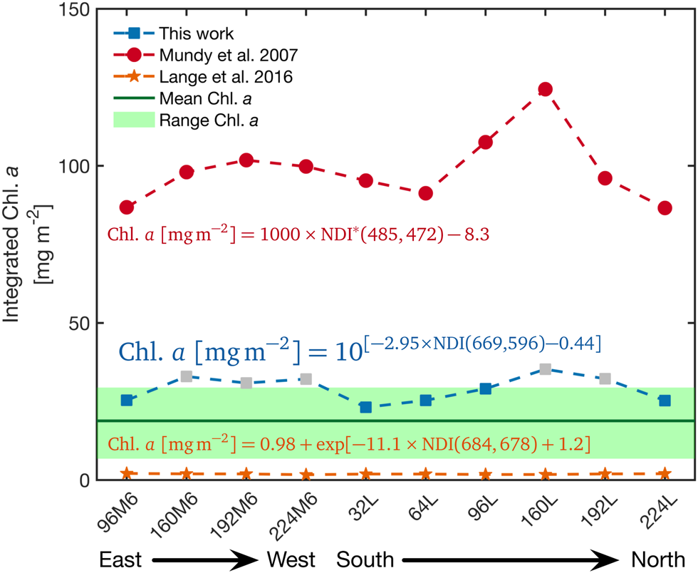
Fig. 8. Comparison of NDI relations. Evaluation of our NDI relationship against the NDI relationships from Mundy and others (Reference Mundy, Ehn, Barber and Michel2007) optimised for thick ice (>1 m) from Resolute Bay, Canadian Arctic and Lange and others (Reference Lange, Katlein, Nicolaus, Peeken and Flores2016) developed from data across the Central Arctic Ocean. Note that the NDI of Mundy and others (Reference Mundy, Ehn, Barber and Michel2007) relationship was calculated from under-ice irradiance from which the relationship was derived (denoted NDI∗ in the figure). The grey boxes indicate the estimated Chl. a concentrations which were higher than the data used to develop the Saroma-ko Lagoon NDI relationship.
The spatial autocorrelation analysis of the horizontal distribution of Chl. a (Fig. 9) showed a Chl. a patchiness of ~65 m (N = 27), a value close to 70 m, which is the smallest patch size reported by Robineau and others (Reference Robineau, Legendre, Kishino and Kudoh1997) for Saroma-ko Lagoon, and also in the same range of 20–90 m as reported by Gosselin and others (Reference Gosselin, Legendre, Therriault, Demers and Rochet1986) for Arctic sea ice in Hudson Bay. Patch sizes of ice thickness, snow depth and freeboard were also estimated from the global significant correlograms and were 75 m, 90 m and 100 m, respectively (Fig. 9).
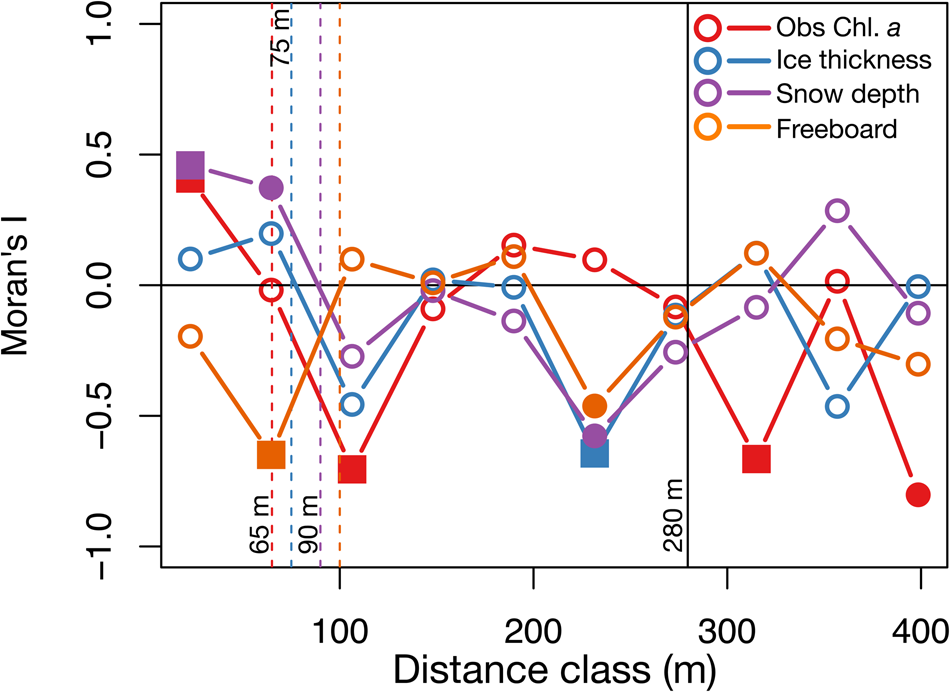
Fig. 9. Spatial analysis. Correlograms or plots of Moran's I versus the distance class of observed Chl. a, ice thickness, snow depth and freeboard (N = 27). Vertical dashed lines indicate patch sizes estimated for each variable were the first zeros of the global significance correlograms were observed, and the vertical solid lines show the truncated range (280 m) to consider in correlograms (2/3 of the maximum distance class, 419 m). Note that solid squares represent p < 0.005 and solid circles represent 0.005 < p < 0.05.
Our suggested Saroma-ko-specific empirical relationship can doubtless be improved. More paired measurements of bio-optical data are needed to improve our relationship, in particular with higher snow and ice thickness variation. Long-term and spatially resolved observations will be crucial to improve our understanding of seasonal and interannual variability of sea-ice algal dynamics and their impacts on light transmission and pelagic biological processes in Saroma-ko Lagoon (Liu and others, Reference Liu, Saitoh, Maekawa, Mochizuki and Tian2018).
Future studies with remotely operate vehicles (ROV) instrumented with CTDs and hyperspectral under-ice irradiance sensors could obtain more data to derive the patchiness of sea-ice algae, similar to the approaches of Meiners and others (Reference Meiners2017) and Lange and others (Reference Lange2017). These ROV studies could also be used to upscale and increase the spatial resolution of ice algal biomass surveys in order to study the physical oceanic controls on sea-ice algal biomass along the salinity gradient (Legendre and others, Reference Legendre, Aota, Shirasawa, Martineau and Ishikawa1991). For the determination of ice algal temporal dynamics, hyperspectral radiometers could be mounted onto buoys or moorings to study the phenology of sea-ice algae in Saroma-ko Lagoon (Liu and others, Reference Liu, Saitoh, Maekawa, Mochizuki and Tian2018), similar to studies previously conducted in the Arctic (Campbell and others, Reference Campbell, Mundy, Barber and Gosselin2015; Hill and others, Reference Hill, Light, Steele and Zimmerman2018).
Conclusions
In summary, our study provides a new NDI to Chl. a relationship to estimate sea-ice algal biomass from transmitted light measurements in Saroma-ko Lagoon, Japan. The observed relationship is comprised of wavelengths in the orange/red wavelength range which is likely attributed to the specific physical and biogeochemical (CDOM) properties of the lagoon's sea-ice cover. This empirical index was compared with two existing Arctic NDI indices and showed that the area-specific index was better suited to estimate ice algal biomass in the lagoon. Spatial analyses showed that the patch size of sea-ice Chl. a was 65 m, similar to estimates from previous studies. Our study also showed that the spatial distribution of Chl. a concentrations in the bottom 0.1 m of the sea-ice cores was significantly correlated with both brine-volume fraction and sea-ice thickness. Our new NDI relationship can be applied to noninvasively estimated land-fast ice algal biomass in Saroma-ko Lagoon, providing a cost-effective approach for monitoring ice algal biomass during the winter and spring transition. A similar approach and empirical relationship may be applied for other low-latitude sea-ice regions but will need validation.
Supplementary material
The supplementary material for this article can be found at https://doi.org/10.1017/aog.2020.69.
Acknowledgements
This study is a contribution to the Saroma-ko Lagoon Observations for sea-ice Physico-chemistry and Ecosystems 2019 (SLOPE2019) project. We are very grateful to Saroma Research Centre of Aquaculture and Napal Kitami for their support in conducting the fieldwork. This work was supported by the Japan Society for the Promotion of Science (17H04715, 17H06322, 17K00534, 18H03745, 18KK0292, and 18F18794). We thank Yusuke Kawaguchi, Takashi Ono, Itsuka S. Yabe, Eun Yae Son, Frederic Vivier, Antonio Lourenco, Marion Lebrun and Martin Vancoppenolle for assistance in the field. We acknowledge two anonymous reviewers, the scientific editor Feiyue Wang and Matthew Corkill, whose suggestions and comments helped improve an earlier version of the manuscript.


 Open access