


1. Introduction
Flows of granular materials such as sand, snow and coal are a common occurrence in nature and in industry. In nature, they occur as avalanches of granular snow, as rock debris slides, and in planetary rings. In industry, they occur in pharmaceutical, mining and polymer processing. Also, in energy production, there are important flows of granular materials in fluidized beds.
Continuum modelling of granular media is motivated by the pioneering experimental work of Bagnold (Reference Bagnold1954, Reference Bagnold1966), which suggested that the transfer of momentum in flows is due to collisions between grains. Later, Jenkins & Savage (Reference Jenkins and Savage1983) extended the kinetic theory of dense gases (Chapman & Cowling Reference Chapman and Cowling1964) to describe the rapid flow of identical, smooth, nearly elastic, spherical particles. At the same time, Haff (Reference Haff1983) presented a continuum description of granular flow using a heuristic theoretical approach. These relatively crude theories have been improved upon by several researchers (Lun et al. Reference Lun, Savage, Jeffrey and Chepurniy1984; Jenkins & Richman Reference Jenkins and Richman1985; Goldshtein & Shapiro Reference Goldshtein and Shapiro1995; Sela, Goldhirsch & Noskowicz Reference Sela, Goldhirsch and Noskowicz1996; Sela & Goldhirsch Reference Sela and Goldhirsch1998).
The first kinetic theory for granular gases by Jenkins & Savage (Reference Jenkins and Savage1983) focused on dense shearing flows of identical, frictionless, nearly elastic, rigid spheres. The collisions were assumed to be instantaneous, binary and uncorrelated. However, discrete element simulations of steady, homogeneous, shearing flows of rigid, frictionless spheres show that velocity correlations do develop at solid volume fractions greater than the freezing point  $0.49$ (Mitarai & Nakanishi Reference Mitarai and Nakanishi2005, Reference Mitarai and Nakanishi2007), and these correlations influence the relationship between the components of stress and shear rate (Mitarai & Nakanishi Reference Mitarai and Nakanishi2007). The freezing point is the lowest value of the volume fraction at which the three-dimensional assembly of rigid spheres can experience a first-order transition to an ordered collisional state, (Torquato Reference Torquato1995). At volume fractions above the freezing point, the granular temperature – a measure of intensity of the particle velocity fluctuations – differs from the strength of the relative velocities between colliding grains (Mitarai & Nakanishi Reference Mitarai and Nakanishi2007), and the assumption of molecular chaos breaks down.
The rate of collisional dissipation in the kinetic theory is most sensitive to the difference between the strengths of the velocity fluctuations and the relative velocities (Mitarai & Nakanishi Reference Mitarai and Nakanishi2005, Reference Mitarai and Nakanishi2007). Because of this, it must be modified in the theory. Jenkins (Reference Jenkins2006, Reference Jenkins2007) did this by introducing a length scale larger than a particle diameter, and used it in the denominator of the collisional rate of dissipation. The length is obtained in a local balance between the orienting influence of the flow and the randomizing influence of collisions (Jenkins Reference Jenkins2007; Jenkins & Berzi Reference Jenkins and Berzi2010).
This extension of the kinetic theory applies until the mean separation distance between the edges of the spheres becomes zero. At this volume fraction, the stress relations for hard spheres become singular (Berzi & Vescovi Reference Berzi and Vescovi2015). Numerical simulations show that this critical volume fraction,  $\nu _c,$ at which the singularity occurs depends on the coefficient of sliding friction. For frictionless spheres, it occurs at random close packing (Torquato Reference Torquato1995); for frictional spheres, it occurs at at a volume fraction less than this (Chialvo, Sun & Sundaresan Reference Chialvo, Sun and Sundaresan2012). With compliant, rather than rigid, spheres, the instantaneous contact is replaced by one of finite duration. Incorporating the duration of contact into the frequency of collision eliminates the singularity at the critical volume fraction. The stresses above this singularity then include two contributions: one that is independent of shear rate, which is associated with the elasticity of the contacts; and one that depends upon shear rate, which is associated with the breaking of force chains (Chialvo et al. Reference Chialvo, Sun and Sundaresan2012).
Granular flows through vertical channels have been of interest for decades. Goodman & Cowin (Reference Goodman and Cowin1971) studied vertical channel flow and observed a plug region existing in the central part of the channel. They also observed that the solid volume concentration in the shearing region outside the plug is affected by the boundary conditions and may either increase or decrease from the plug to the channel wall. The shearing zones occurred in many other studies (Nedderman & Laohakul Reference Nedderman and Laohakul1980; Mohan, Nott & Rao Reference Mohan, Nott and Rao1997; Pouliquen, Forterre & Le Dizes Reference Pouliquen, Forterre and Le Dizes2001). Savage (Reference Savage1979) proposed a constitutive equation, an extension to the continuum theory of Goodman & Cowin (Reference Goodman and Cowin1972), for the flow of cohesionless granular materials at high deformation rates and low stress levels. In experiments on two-dimensional shear flows that corresponded to their analyses, fibre optic probes were used to measure the velocity profiles to compare with the predictions. Ananda, Moka & Nott (Reference Ananda, Moka and Nott2008) studied the dense, slow flow of granular materials through vertical channels using video imaging and particle tracking to determine the profiles of mean velocity across a range of different channel widths. Mohan, Nott & Rao (Reference Mohan, Nott and Rao1999) used a rigid-plastic Cosserat model to study dense, fully developed flows of granular materials through a vertical channel. The Cosserat model predicted the variation of the velocity profiles and the variation of the thickness of the shear layer with the width of the channel.
Despite these and other studies of granular flow through vertical channels and hoppers (Gudhe, Yalamanchili & Massoudi Reference Gudhe, Yalamanchili and Massoudi1994; Natarajan, Hunt & Taylor Reference Natarajan, Hunt and Taylor1995; Wang, Jackson & Sundaresan Reference Wang, Jackson and Sundaresan1997) and recent discrete element method (DEM) studies (Zhao et al. Reference Zhao, Yang, Zhang and Chew2018; González-Montellano, Ayuga & Ooi Reference González-Montellano, Ayuga and Ooi2011; Barker, Zhu & Sun Reference Barker, Zhu and Sun2022; Debnath, Kumaran & Rao Reference Debnath, Kumaran and Rao2022a), the flow through a vertical channel still lacks a clear understanding, especially in the rapid flow regime where grains interact through collisions and experience free flight between consecutive encounters. The extended kinetic theory (EKT) permits an understanding of steady, inhomogeneous, collisional, granular shearing flows that range from dilute to dense concentrations, and allows the predictions of profiles of solid volume fraction and particle mean and fluctuation velocity in terms of a small number of measurable parameters.
In this work, we consider steady, fully-developed, gravity-driven, inhomogeneous shearing flows of soft, frictional spheres in a vertical chute that is bounded by two bumpy walls. We use the EKT, outlined by Berzi, Jenkins & Richard (Reference Berzi, Jenkins and Richard2020) for the granular flow outside and within a vertical erodible bed, to study the flow in the chute. When the solid volume fraction at the centreline exceeds a critical value, we employ the model for the bed, which combines the rate-independent elastic transfer of force through continuous chains of particles, and the rate-dependent mechanism of collisional momentum transfer that results from their breaking. We employ only the rate-dependent components of stresses in the regions of the flow below the critical volume fraction. We adopt boundary conditions derived by Richman (Reference Richman1988) for parallel bumpy boundaries with hemispheres attached to them. When a sufficient amount of spherical particles are fed to the chute, a dense region, analogous to an erodible bed, develops around the centreline of the chute. In this case, continuity conditions are also applied at the surface of the bed.
2. Flow configuration, regimes and constitutive relations
A schematic diagram of the chute is shown in figure 1. We consider the flow of identical spheres of mass density  $\rho _s$ and diameter $d$, driven between two rigid, bumpy boundaries, separated by distance $2R$, by the gravitational acceleration $\boldsymbol {g}$. The directions $x$,
$x$,  $y$ and $z$ are along the chute, across the chute, and out of the plane, respectively. In the steady fully developed flow, the flow is independent of $x$ and time. Also, it is assumed that the flow is of infinite extent in $z$ direction. Consequently, there is no variation of the flow along the $z$ direction, and all quantities vary with $y$ alone. The only non-zero component of the mean velocity is $u$, in the $x$ direction. Boundary conditions on the shear stress and energy flux are applied at the rigid, bumpy boundary and at the centreline of the flow. We define the partial volume flow rate across the half-width of the chute as $I(y) = \int _{0}^{y}\nu u \,{\rm d} y$, which permits us to use the total volume flow rate $Q$ as one of the boundary conditions. The erodible bed extends along the $x$ axis, contains the centreline of the chute, and has width $h_2$, where $-h_2 \le y \le 0$; the collisional flow extends along the $x$ axis and has width $h_1$, where $0\le y\le h_1$. As in Berzi, Jenkins & Richard (Reference Berzi, Jenkins and Richard2019), we assume that for $\nu > \nu _c$, an erodible bed forms that consists of spheres in chains of ephemeral contact along the axis of greatest compression that when breaking, create collisions. In the flow between the bed and the bumpy wall, the solid volume fraction is less than $\nu _c$; the flow particles interact through collisions, and experience free flight between the successive encounters.
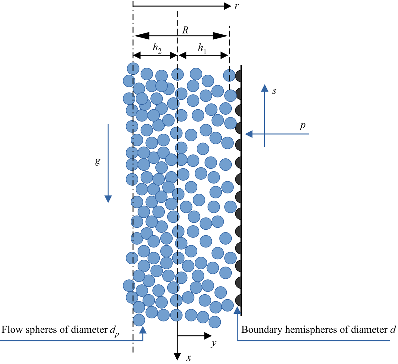
Figure 1. Schematic of the chute. Here,  ${g}$ is the gravitational acceleration, and ${p}$ and ${s}$ are the pressure and shear stress, respectively, exerted by the boundary on the flow. In the erodible bed, $-h_2\le y \le 0$, and $\nu > \nu _c$; the collisional flow is outside the bed.
For compliant contacts between the particles, the duration of particle contact is not zero and, with increasing compliance, the frequency of collisions must decrease. Berzi & Jenkins (Reference Berzi and Jenkins2015) capture this quantitatively by taking the frequency of collisions to be inversely proportional to the sum of time of free flight between collisions and the duration of contact. The ratio of free flight to the sum of time of free flight  $t_f$ and contact duration $t_c$ is given as (Berzi & Jenkins Reference Berzi and Jenkins2015)
 \begin{equation} \frac{t_f}{t_f+t_c}= \frac{{\rm \pi}^{1/2}}{24}\,\frac{d}{G T^{1/2}} \left(\frac{{\rm \pi}^{1/2}}{24}\,\frac{d}{G T^{1/2}} + \frac{d}{5c_o}\right)^{{-}1}, \end{equation}
where
 \begin{equation} t_f=\frac{{\rm \pi}^{1/2}}{24}\,\frac{d}{G T^{1/2}}. \end{equation}
The duration of a collision contact is proportional to the ratio of the particle diameter to the elastic wave speed in the particle,  $c_o= ({E}/{\rho _s}$), where $E$ is the Young's modulus of the material of the spheres (Hwang & Hutter Reference Hwang and Hutter1995). Here and elsewhere, the granular temperature $T$ is a measure of the strength of velocity fluctuations, and $G=\nu g_0$ is the product of solid volume fraction $\nu$ and radial distribution function $g_0$. The radial distribution function contains information about the probability of having two particles at close contact and hence incorporates the influence of the volume occupied by the flow particles on the collision frequency. The collisional stress, the collisional rate of dissipation of fluctuation energy, and the flux of fluctuation energy are all proportional to the frequency of collisions. So for the soft particles, the relations given by the kinetic theory for rigid spheres must be multiplied by the ratio of (2.1) (Berzi & Jenkins Reference Berzi and Jenkins2015; Berzi et al. Reference Berzi, Jenkins and Richard2020).
2.1. Constitutive relations and flow regimes
In the following, we introduce the constitutive relations for the flow regions. More details can be found in (Garzó & Dufty Reference Garzó and Dufty1999; Berzi & Jenkins Reference Berzi and Jenkins2015; Berzi et al. Reference Berzi, Jenkins and Richard2020). All quantities are made dimensionless using the mass density and diameter of the spheres, and the gravitational acceleration. For the sake of simplicity, the notation for the dimensionless variables remains the same.
2.1.1. Collisional flow
In the collisional flow regime,  $0\le y \le h_1,$ $\nu < \nu _c$, the mean inter-particle distance is greater than zero and the stresses develop due to momentum exchange between and during collisions. The resulting expressions for the pressure and shear stress are
 \begin{equation} p= f_1 T\left(1+\frac{12}{5}\,G\,\frac{T^{1/2}}{k_n^{1/2}}\right)^{{-}1} \end{equation}
and
 \begin{equation} s= f_2 T^{1/2}\left(1+\frac{12}{5}\,G\,\frac{T^{1/2}}{k_n^{1/2}}\right)^{{-}1}u', \end{equation}
where the prime indicates a derivative with respect to  $y$, the correction term due to the non-zero contact duration includes the dimensionless spring stiffness $k_n$ in the spring–dashpot simulation model for the contact (Ji & Shen Reference Ji and Shen2008; Chialvo et al. Reference Chialvo, Sun and Sundaresan2012; Chialvo & Sundaresan Reference Chialvo and Sundaresan2013), and the auxiliary coefficients $f_1$ and
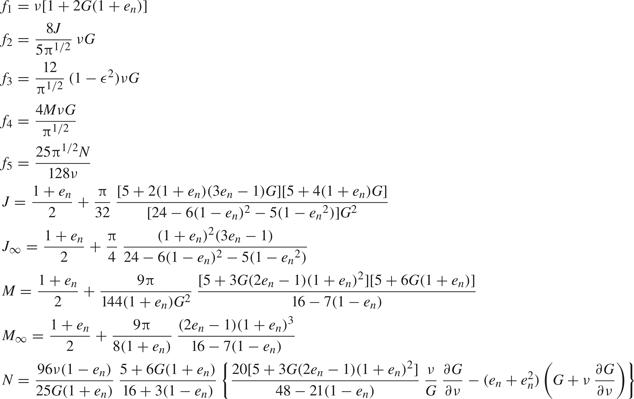
  $f_2$ are given in table 1. The dimensional form of $k_n$ is the product of $E$ and $d$. The coefficient $f_1$ contains the coefficient of normal restitution $e_n$.
Table 1. Coefficients used in constitutive relations of EKT.
For the radial distribution function  $g_0$, we use the expression suggested by Vescovi et al. (Reference Vescovi, Berzi, Richard and Brodu2014): for $\nu <0.4$,
 \begin{equation} g_0 = \frac{2-\nu}{2(1-\nu)^3}, \end{equation}
and for  $0.4 \leq \nu < \nu _c$,
 \begin{equation} g_0 =\left[ 1- \left(\frac{\nu -0.4}{\nu_c -0.4}\right)^2 \right] \frac{2- \nu}{2(1-\nu)^3}+ \left(\frac{\nu -0.4}{\nu_c -0.4}\right)^2 \frac{2}{\nu_c-\nu} . \end{equation}
The coefficients  $f_1$ and $f_2$ are proportional to $G$, so when $\nu$ approaches $\nu _c$, $G$ tends to infinity. If the particles are rigid, then shearing ceases at the critical volume fraction and the system is said to be jammed. However, if the contacts are compliant, then the dimensionless stresses remain finite at $\nu =\nu _c$, because of the modification of the collisional frequency that includes $G$.
$G$.
For the rate of collisional dissipation  $\gamma$, and the flux of fluctuation energy $q$, we use the expressions suggested by Berzi et al. (Reference Berzi, Jenkins and Richard2019):
 \begin{equation} \gamma= \frac{f_3}{L}\,T^{3/2}\left(1+\frac{12}{5}\,G\,\frac{T^{1/2}}{k_n^{1/2}}\right)^{{-}1} \end{equation}
and
 \begin{equation} q={-}f_4 T^{1/2}\left(1+\frac{12}{5}\,G\,\frac{T^{1/2}}{k_n^{1/2}}\right)^{{-}1}T' - f_5 T^{3/2}\left(1+\frac{12}{5}\,G\,\frac{T^{1/2}}{k_n^{1/2}}\right)^{{-}1}\nu' , \end{equation}
where
 \begin{equation} L = \max\left(1, f_0\,\frac{|u'|}{T^{1/2}}\right) \end{equation}
is the correlation length suggested by Jenkins (Reference Jenkins2007). It introduces a decrease in the collisional dissipation rate associated with the velocity correlations that develop at volume fractions greater than freezing (Jenkins Reference Jenkins2007; Mitarai & Nakanishi Reference Mitarai and Nakanishi2007). The coefficients  $f_3$, $f_4$ and $f_5$ are given in table 1. An effective coefficient of restitution $\epsilon$, which incorporates both the normal restitution $e_n$ and the coefficient of sliding friction $\mu$, is introduced to account for energy loss and exchange created by surface friction. The effective coefficient includes frictional dissipation and the exchange of translational and rotational fluctuation energy in the collisional rate of dissipation of translational fluctuation energy, and is employed in the function $f_3$ (Jenkins & Zhang Reference Jenkins and Zhang2002; Berzi & Vescovi Reference Berzi and Vescovi2015; Gollin, Berzi & Bowman Reference Gollin, Berzi and Bowman2017). A simple expression for its dependence on $\mu$ results from the numerical simulations by Chialvo & Sundaresan (Reference Chialvo and Sundaresan2013):
 \begin{equation} \epsilon=e_n-\frac{3}{2}\,\mu \exp{-3 \mu}. \end{equation}
Finally, the coefficient  $f_0$ in the expression (2.9) for the correlation length is given by Berzi & Vescovi (Reference Berzi and Vescovi2015) as
 \begin{equation} f_0 = \left[\frac{2J}{15(1-\epsilon^2)} \right]^{1/2} \left[1+\frac{26(1-\epsilon)(\nu -0.49)}{15(0.64-\nu)} \right]^{3/2}. \end{equation}
2.1.2. Erodible bed
When the volume fraction is larger than the critical volume fraction, the stress components develop a rate-independent contribution associated with the transmission of force through the compliant contacts of an evolving network. A rate-dependent contribution is associated with the breaking of these force chains. In this case, the pressure in the bed is given by Berzi et al. (Reference Berzi, Jenkins and Richard2020) as
 \begin{equation} p = \frac{5}{6}\,(1+e_n)\nu k_n^{1/2} w + 0.0006(\nu - \nu_c)k_n , \end{equation}
and the shear stress is (Berzi & Jenkins Reference Berzi and Jenkins2015; Berzi et al. Reference Berzi, Jenkins and Richard2020)
 \begin{equation} s = \frac{4 J_\infty}{5 {\rm \pi}^{1/2}(1+e_n)}\,\frac{u'}{w}\,p, \end{equation}
where  $J_{\infty }$ is given in table 1, and $w=\sqrt {T}$ is called the fluctuation velocity.
Because collisions persist in the weak, dense, shearing flows in the bed, energy is dissipated and transferred. The collisional dissipation rate  $\gamma$, and the energy flux $q$, in the bed are given by Berzi & Jenkins (Reference Berzi and Jenkins2015) and Berzi et al. (Reference Berzi, Jenkins and Richard2020) as
 \begin{equation} \gamma=\frac{5(1-\epsilon^2) \nu}{{\rm \pi}^{1/2} L_c}\,k_n ^{1/2} T \end{equation}
and
 \begin{equation} q ={-} \frac{5M_\infty \nu}{3{\rm \pi}^{1/2}}\,k_n ^{1/2} T' , \end{equation}
where  $M_{\infty }$ is given in table 1, and $L_c$ is the chain length in the bed:
 \begin{equation} L_c = 1+\frac{26(1-\epsilon)}{15} \frac{\nu_c - 0.49}{0.64-\nu_c}. \end{equation}
3. Governing differential equations for the flow through the chute
The balance equations of mass, momentum and fluctuation energy are used to determine the fields of the average density  $\rho$, the mean velocity $\boldsymbol {u}$, and the granular temperature $T$. These balance laws have the familiar forms
 \begin{gather} \dot \rho + \rho u_{i,i} = 0, \end{gather}
 \begin{gather}\rho \dot u_{i}=\sigma_{ik,k}+nF_{i}, \end{gather}
where  ${\boldsymbol{\sigma} }$ is a symmetric stress tensor, $n$ is the average particle number density, and $\boldsymbol {F}$ is the external force per particle, and
 \begin{align} \tfrac{3}{2}\,\rho \dot T={-}q_{i,i}+ \sigma_{ik}D_{ik}-\gamma, \end{align}
where  $\boldsymbol {q}$ is the flux of fluctuation energy, $\boldsymbol {D}$ is the symmetric part of the velocity gradient tensor, and $\gamma$ is the collisional rate of fluctuation energy per unit volume. Here, an overdot denotes the material time derivative, $D({\cdot })/Dt = \partial ( {\cdot })/\partial t + \boldsymbol {u} \boldsymbol {{\cdot }} \boldsymbol {\nabla }({\cdot })$.
We employ these balance equations together with the constitutive relations introduced in § 2 for a steady fully developed flow through a vertical chute. As mentioned earlier, there is no variation of the flow along  $x$ and $z$, or with time. Therefore, all the quantities vary only with $y$:
$y$:
 \begin{gather} u_{y} = u_{z} = 0,\quad u_x \equiv u(y), \quad F_{z}=F_{y}=0, \quad F_x = \nu, \end{gather}
 \begin{gather}\sigma_{xx}=\sigma_{yy}=\sigma_{zz}={-}p, \end{gather}
 \begin{gather}\sigma_{zx}=\sigma_{yz}=0, \quad \sigma_{xy} \equiv s(y), \end{gather}
 \begin{gather}q_{z}= q_{x}=0, \quad q_{y} \equiv q(y). \end{gather}
3.1. Collisional flow
In the collisional flow, the mass balance (3.1) is satisfied identically, and the momentum balance (3.2) and the energy balance (3.3) become
 \begin{gather} p'=0, \end{gather}
 \begin{gather}s'={-}\nu \end{gather}
and
 \begin{align} q'=su'-\gamma. \end{align}
Differentiating (2.3) with respect to  $y$, and using it in (3.8) and (2.8), results in the differential equation for the volume fraction:
 \begin{equation} \nu ' = \left[ \frac{\partial p}{\partial T}\left(1+\frac{12}{5}\,G\, \frac{T^{1/2}}{k_n^{1/2}}\right)q \right] \left( \frac{\partial p}{\partial \nu}\,f_4 w - \frac{\partial p}{\partial T}\,f_5 w^3\right)^{{-}1}, \end{equation}
where
 \begin{equation} \frac{\partial p}{\partial T}= f_1 \left(1+\frac{12}{5}\,G\,\frac{T^{1/2}}{k_n^{1/2}}\right)^{{-}1} - \frac{1}{2}\,f_1\,\frac{12}{5}\,G\,\frac{w}{k_n^{1/2}} \left(1+\frac{12}{5}\,G\, \frac{T^{1/2}}{k_n^{1/2}}\right)^{{-}2} \end{equation}
and
 \begin{equation} \frac{\partial p}{\partial \nu}= \frac{\partial f_1}{\partial \nu}\,w^2 \left(1+\frac{12}{5}\,G\, \frac{T^{1/2}}{k_n^{1/2}}\right)^{{-}1} - f_1 w^2\,\frac{12}{5}\,\frac{\partial G}{\partial \nu}\, \frac{w}{k_n^{1/2}} \left(1+\frac{12}{5}\,G\,\frac{T^{1/2}}{k_n^{1/2}}\right)^{{-}2}. \end{equation}
The differential equation for the shear stress is given in (3.9). Inverting (2.4) provides the differential equation for the mean velocity:
 \begin{equation} u' = \frac{1}{f_2}\,\frac{s}{w}\left(1+\frac{12}{5}\,G\,\frac{T^{1/2}}{k_n^{1/2}}\right). \end{equation}
The differential equation for energy flux is obtained from the balance of fluctuation energy (3.10):
 \begin{equation} q' = \frac{1}{f_2}\,\frac{s^2}{w}\left(1+\frac{12}{5}\,G\,\frac{T^{1/2}}{k_n^{1/2}}\right) - \frac{f_3}{L}\,w^3 \left(1+\frac{12}{5}\,G\,\frac{T^{1/2}}{k_n^{1/2}}\right)^{{-}1}. \end{equation}
The differential equation for the fluctuation velocity is obtained by inverting (2.8) and using (3.11):
 \begin{align} w' &={-} \frac{q}{2 f_4 w^2} \left(1+\frac{12}{5}\,G\,\frac{T^{1/2}}{k_n^{1/2}}\right) - \frac{f_5}{2 f_4}\,w \left[ \frac{\partial p}{\partial T}\left(1+\frac{12}{5}\,G\,\frac{T^{1/2}}{k_n^{1/2}}\right)q \right]\nonumber\\ &\quad \times \left( \frac{\partial p}{\partial \nu}\,f_4 w - \frac{\partial p}{\partial T}\,f_5 w^3\right)^{{-}1}. \end{align}
Finally, the differential equation for the volume flow rate is
 \begin{equation} I'=\nu u. \end{equation}
3.2. Erodible bed
In the bed, the momentum balances (3.8) and (3.9) are the same as in the collisional flow. However, because the energy produced by the working of the shear stress is assumed to be small compared to its diffusion and dissipation, the energy balance is
 \begin{equation} {-q'}=\gamma . \end{equation}
The differential equation governing the flow in the bed for the solid volume fraction is obtained by differentiating (2.12) and using (3.8) and (2.15):
 \begin{equation} \nu ' = \left [ \frac{{\rm \pi}^{1/2}(1+e_n)q}{4M_\infty w}\right] \left [ \frac{5}{6}\,(1+e_n) k_n^{1/2} w + 0.0006 k_n\right]^{{-}1}. \end{equation}
The rate of shear in the bed is obtained from (2.13) and (2.12) as
 \begin{equation} u ' = \left [ \frac{5{\rm \pi}^{1/2}(1+e_n)}{4J_\infty }\,s w\right] \left [ \frac{5}{6}\,(1+e_n) \nu k_n^{1/2} w + 0.0006(\nu - \nu_c) k_n\right]^{{-}1}. \end{equation}
The differential equation for the energy flux is obtained using (3.18) and (2.14):
 \begin{equation} q'={-}\frac{5(1-\epsilon^2) \nu}{{\rm \pi}^{1/2} L_c}\,k_n ^{1/2} T. \end{equation}
The differential equation for the fluctuation velocity in the bed is obtained from (2.15):
 \begin{equation} w' ={-} \frac{3{\rm \pi}^{1/2}q}{10 \nu M_\infty k_n^{1/2}w}. \end{equation}
Finally, the volume flow rate is again governed by (3.17).
4. Boundary conditions
We use boundary conditions for slip velocity and energy flux at a wall made bumpy with frictionless hemispheres, derived by Richman (Reference Richman1988), in their simplest form. More complicated expressions for the influence of geometric features on slip and energy flux are available in Richman (Reference Richman1988) and Jenkins (Reference Jenkins1998, Reference Jenkins2001). The boundary condition for the slip velocity results from the balance of momentum in the flow direction:
 \begin{equation} \frac{u_b}{w_b}= \left(\frac{\rm \pi}{2}\right)^{1/2} f\,\frac{s_b}{p_b}, \end{equation}
where the subscript  $b$ refers to the boundary, and
 \begin{equation} f = \left[ \frac{3}{2^{5/2} J_{b}}\,\frac{2^{3/2}J_{b}-5F_b(1+B) \sin^2 \theta}{2(1-\cos\theta)/\sin^2 \phi -\cos \theta}+\frac{5F_b}{2^{1/2} J_b}\right], \end{equation}
in which the bumpiness  $\theta$ measures the average maximum penetration of a flow sphere between boundary spheres. When the diameter of the boundary spheres is the same as that of the flow spheres, the bumpiness is given by $\sin \theta = (d+l)/2 d$, where $l$ is the separation between the edges of the boundary spheres, $B = {\rm \pi}[1+5/(8G_b) ]/(12 \sqrt {2})$, and $F_b=(1+e_n)/2+ 1/(4G_b)$. The boundary condition for the energy flux is
 \begin{equation} q_b= s_b u_b - D, \end{equation}
where  $D$ is the collisional rate of dissipation of fluctuation energy at the bumpy wall:
 \begin{equation} D= \left( \frac{2}{\rm \pi} \right)^{1/2} \frac{p_b w_b}{L_b}\,(1-\epsilon) \frac{2(1-\cos \theta)}{\sin^2 \theta}, \end{equation}
in which, for consistency with the EKT, the correlation length and the effective coefficient of restitution are included in the expression for collisional rate of dissipation. The chain length  $L_b$ incorporates the correlations at the boundary.
Other boundary conditions are the vanishing of the shear stress and the energy flux at the centreline of the chute, the specification of  $\nu =\nu _c$, and the continuity of $s$,
$s$,  $u$,
$u$,  $q$,
$q$,  $w$ and $I$ at the interface between the bed and collisional flow region, and the specification of the total flux $Q$.
$Q$.
5. Results and discussion
We solve the system of 12 differential equations (3.11), (3.14), (3.19), (3.20) and (3.9) for the 12 unknown variables  $\nu$, $s$,
$s$,  $u$,
$u$,  $q$,
$q$,  $w$ and $I$ in the collisional flow region and in the erodible bed. We use the Matlab solver ‘bvp4c’ for the two-point boundary-value problem with 12 differential equations and 14 boundary conditions, assuming continuity in all six variables at the interface between collisional flow and the bed. The two additional boundary conditions enable us to determine the thicknesses $h_1$ of the collisional flow and the pressure for a given total flow rate. Alternatively, when pressure is given as an input, the total flow rate $Q$ is obtained as part of a solution. The solver iterates the solutions from an initial guess and carries out mesh refinement, if necessary, to satisfy the boundary conditions. The relative tolerance and absolute tolerance employed are $10^{-6}$ and $10^{-8}$, respectively. We take $k_n=3\times 10^6$, $\mu =0.15$, $e_n=0.85$ and $\theta ={\rm \pi} /5$, unless specified otherwise. Also, to be consistent with the dependence of $\nu _c$ with $\mu$ (Chialvo et al. Reference Chialvo, Sun and Sundaresan2012), we have used the expression for the critical solid volume fraction as $\nu _c=0.587 +(0.636-0.58)\exp {-4.5 \mu }$.
In figure 2, we show the profiles of  $\nu$, $s$,
$s$,  $u$ and $w$ from the centre of the chute to the bumpy wall, for the total flow rate $Q=250$ and two half chute widths, $R = 14$ and 16. For a given total flow rate, the width $h_2$ of the erodible bed and the volume fraction in the collisional flow increase as the chute width increases. Consequently, the mean velocity and the granular temperature in the chute decrease with its increasing width. The shear stress does not show a significant change with $R$. The volume fraction, mean velocity and fluctuation velocity remain nearly constant in and near the erodible bed; but away from the bed, they vary significantly. Moreover, the granular temperature, which is measured by the fluctuation velocity, remains close to zero in the erodible bed and in the collisional region close to the bed. The granular temperature increases towards the bumpy boundary. This variation results from the enhanced collisions away from the erodible bed due the presence of the bumpy wall.
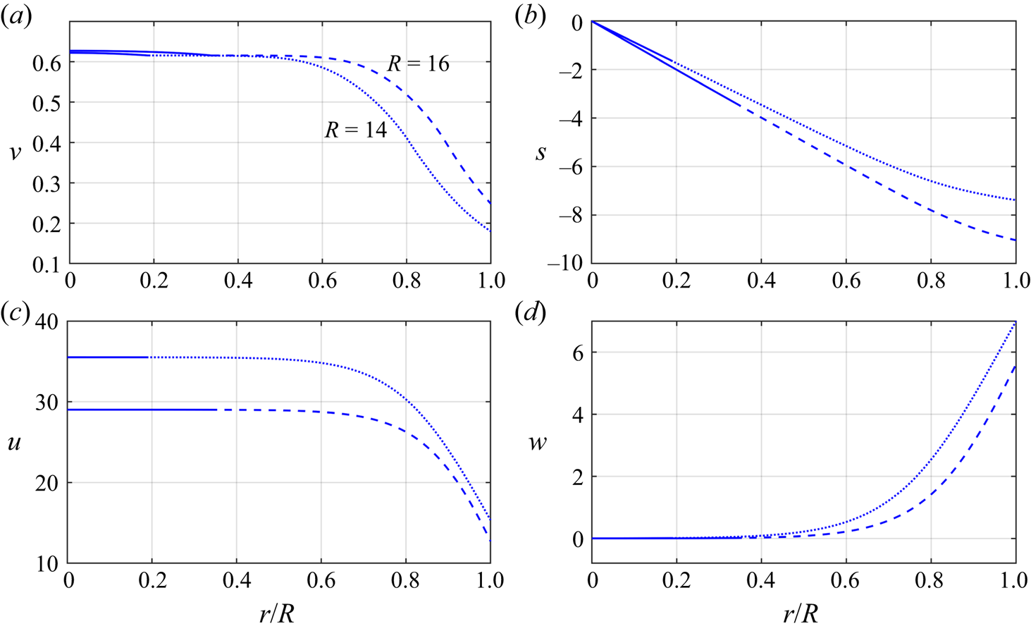
Figure 2. Profiles of (a)  $\nu$, (b) $s$, (c) $u$, and (d) $w$, at different chute widths $R$, and total flow rate $Q = 250$. Here, $r/R$ is the scaled distance from the centre of the chute. The thicker solid lines indicate the erodible bed, the width of which, $h_2$, increases with chute width.
To further illustrate the properties of the collisional flow, in figure 3 we present the variation with the total flow rate  $Q$ of the pressure $p$ (figure 3a), average solid volume fraction $\bar {\nu }_{coll} = \int _{0}^{h_1} \nu \, {\rm d} y/h_1$ (figure 3b), average mean velocity $\bar {u}_{coll}=\int _{0}^{h_1} u\, {\rm d} y/h_1$ (figure 3c), average fluctuation velocity $\bar {w}_{coll} = \int _{0}^{h_1} w\, {\rm d} y/h_1$ (figure 3e) and thickness $h_1$ (figure 3d) of the collisional flow, and average mean velocity $\bar {u}_{bed}=\int _{0}^{h_2} u\, {\rm d} y/h_2$ (figure 3f) in the erodible bed, for four different chute widths, $R=10$, 12, 14 and $16$. In the erodible bed, the solid volume fraction is close to its critical value $\nu _c$, and the average fluctuation velocity is almost zero (not shown). For a given chute width, the average volume fraction, and consequently the pressure in the collisional flow, decreases with the total flow rate, whereas the average mean velocities $\bar u_{coll}$ and $\bar u_{bed}$ in both regions and the width of the collisional flow $h_1$ all increase. Further, the average mean velocity in the bed is slightly higher than that in the collisional flow. For a given chute width, a smaller total flow rate involves fewer particles in collisions with the bumpy boundary. This is manifested by a wider bed and a narrower collisional region (figure 3d), and low fluctuation velocity (figure 3e) in the collisional region.
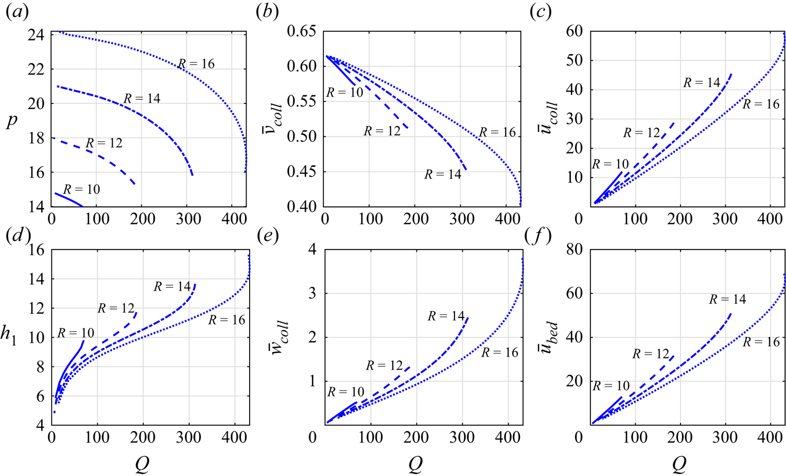
Figure 3. Variation with the total flow rate  $Q$ of (a) pressure $p$, (b) average solid volume fraction $\bar {\nu }_{coll}$, (c) average mean velocity $\bar {u}_{coll}$, and (d) collisional flow width $h_1$. (e) Average fluctuation velocity $\bar {w}_{coll}$ in the collisional flow. (f) Average mean velocity $\bar {u}_{bed}$ in the erodible bed.
Flow through the chute resembles a plug flow. As the total flow rate increases, more particles collide in the bumpy wall, resulting in momentum influx, which in turn promotes further collisions in the chute, leading to higher average fluctuation velocity, lower average volume fraction in the collisional flow, and a larger difference between the average mean velocities of the bed and the collisional flow (not shown, but can be inferred from figures 3c,f). Further, the enhanced collisions erode the bed and the width of the collisional flow increases. Eventually, as indicated in figure 3(d), there is a total flow rate at which the width of the collisional flow,  $h_1$, is almost equal to the chute width. Above this total flow rate, the entire chute experiences collisional flow and the bed vanishes.
Because, for any particular chute width, the bed vanishes beyond a total flow rate, we reformulate the problem without the bed and solve the governing equations for the collisional flow only. The system consists of the six differential equations for the collisional flow and the associated boundary conditions. In figure 4, we show the variation with total flow rate of the average volume fraction and average mean velocity in the collisional region across the chute with and without an erodible bed. In figure 5, we plot the variation with total flow rate of the pressure in the two types of flow. In the collisional flows with a bed, there is a decrease of  $\bar \nu _{coll}$ and $p$, and an increase of $\bar u_{coll}$ with increasing total flow rate, as mentioned earlier. The same trend continues in the fully collisional flow after the bed vanishes, up to a certain total flow rate that depends on the chute width. Beyond this flow rate, no steady solutions exist. However, below this critical value of the total flow rate, another purely collisional solution branch exists for any chute width. On this branch, $\bar \nu _{coll}$, $\bar {u}_{coll}$ and $p$ increase with an increase in total flow rate, up to a critical total flow rate, as observed in figures 4 and5. The two solution branches meet at the critical total flow rate. We note that there are values of $Q$ and $R$ for which there are two purely collisional flows.
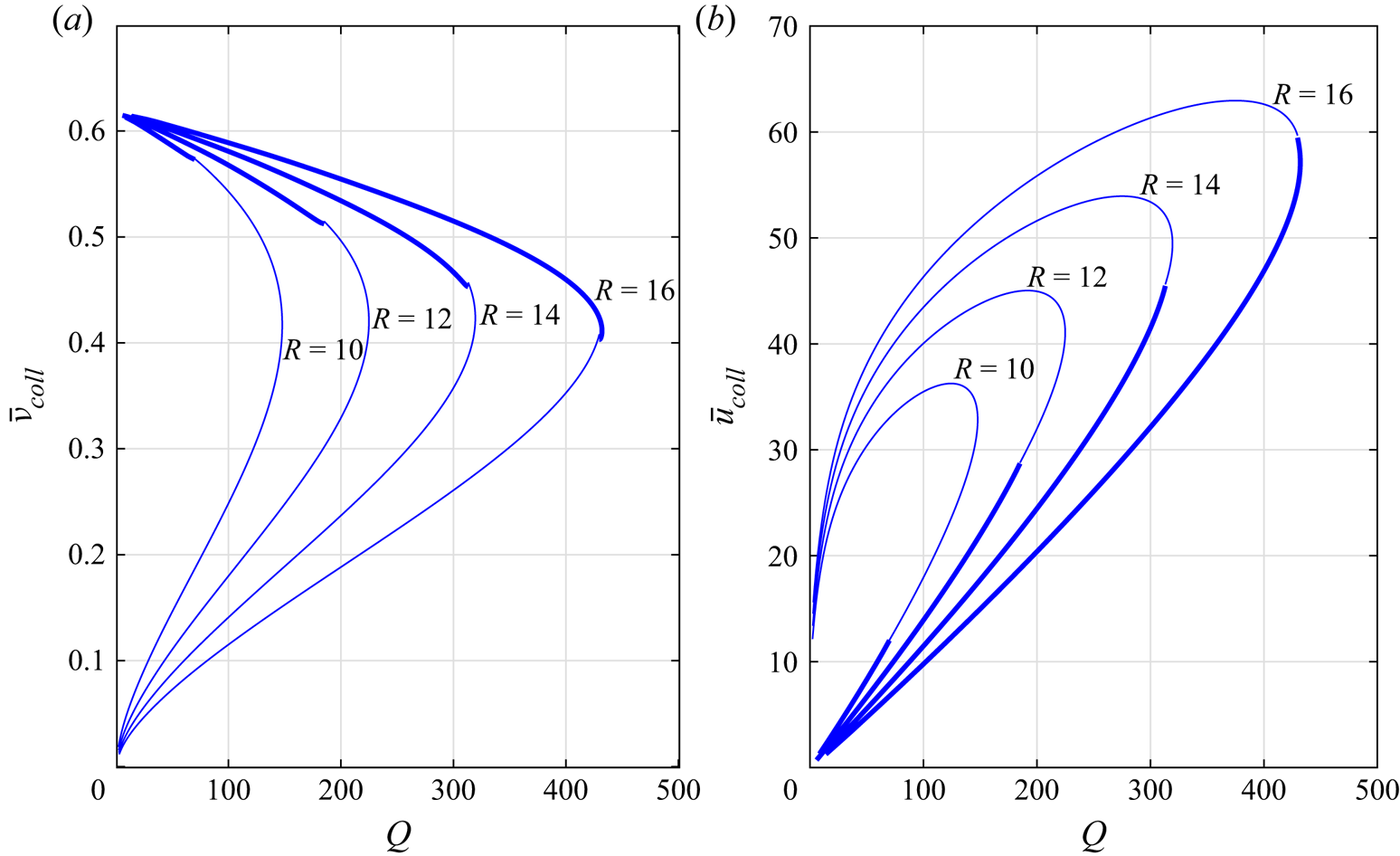
Figure 4. Variation with the total flow rate  $Q$ of (a) average solid volume fraction $\bar {\nu }_{coll}$, and (b) average mean velocity $\bar {u}_{coll}$. The thick lines indicate collisional flows with a bed; the thin lines indicate the collisional flows without a bed. The curves for both types of flow meet.
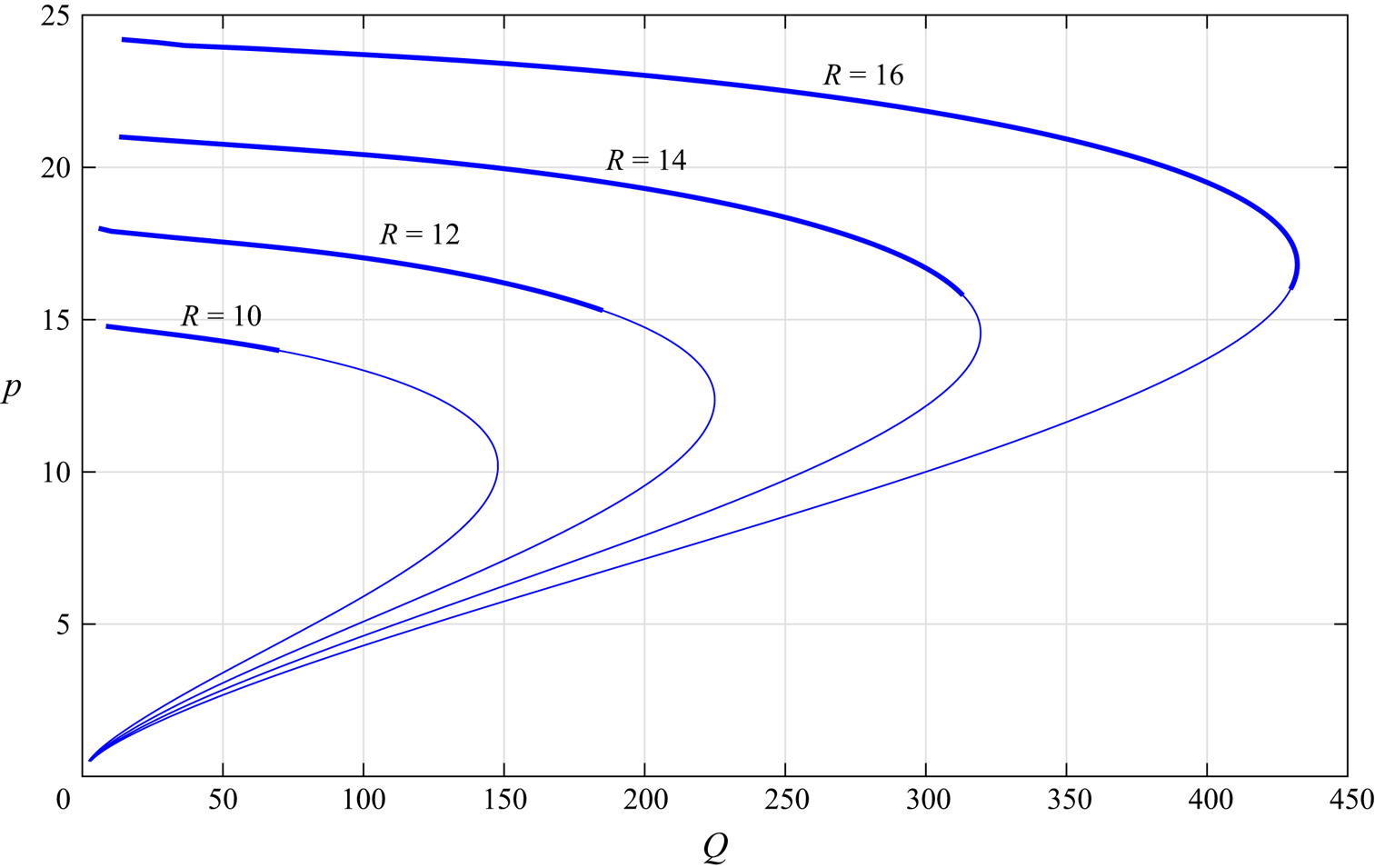
Figure 5. Variation of pressure  $p$ with the total flow rate $Q$ for different chute widths $R$. The thick lines indicate collisional flows with a bed; the thin lines indicate the collisional flows without a bed. The curves for both types of flow meet.
In figures 6 and 7, we show representative profiles of  $\nu$, $s$,
$s$,  $u$ and $w$ over the half chute width of two solutions, with and without bed, respectively, at $Q=150$, and $R=12$ and $14$. The solution with the higher pressure exhibits relatively denser flow with lesser velocity, while the solution branch with lower pressure exhibits comparatively lesser concentration along with higher mean velocity. Also, in figure 8, we provide profiles of $\nu$, $s$,
$s$,  $u$ and $w$ at $Q=150$ and $R=14$ for solutions on the branches with higher and lower pressures.
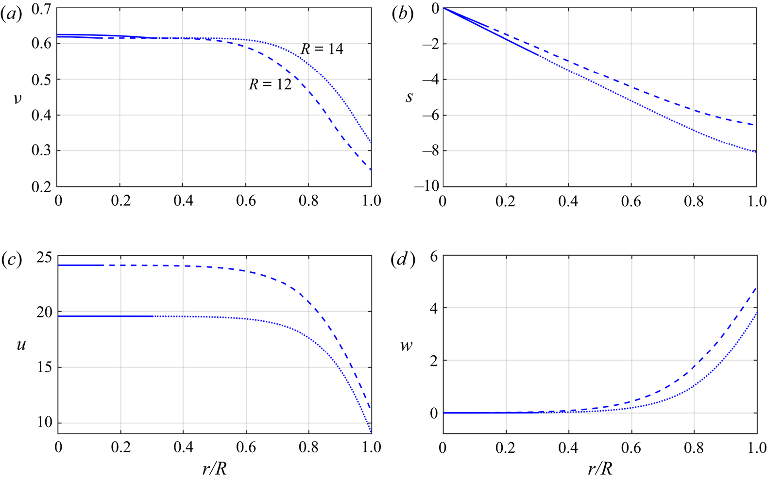
Figure 6. Profiles of (a)  $\nu$, (b) $s$, (c) $u$, and (d) $w$, for $Q=150$, and $R=12$ and $14$, for solutions on the high-pressure branch. These include both an erodible bed and a collisional flow. The solid lines indicate the erodible bed, the width of which increases with the width of the chute.
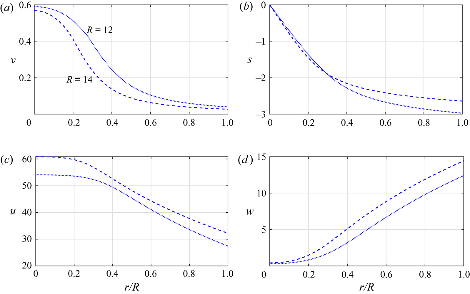
Figure 7. Profiles of (a)  $\nu$, (b) $s$, (c) $u$, and (d) $w$, for $Q=150$, and $R=12$ and $14$, for solutions on the low-pressure branch. Flows on this branch are fully collisional and are characterized by a smaller concentration and a higher mean velocity than those on the high-pressure branch (cf. figure 6).
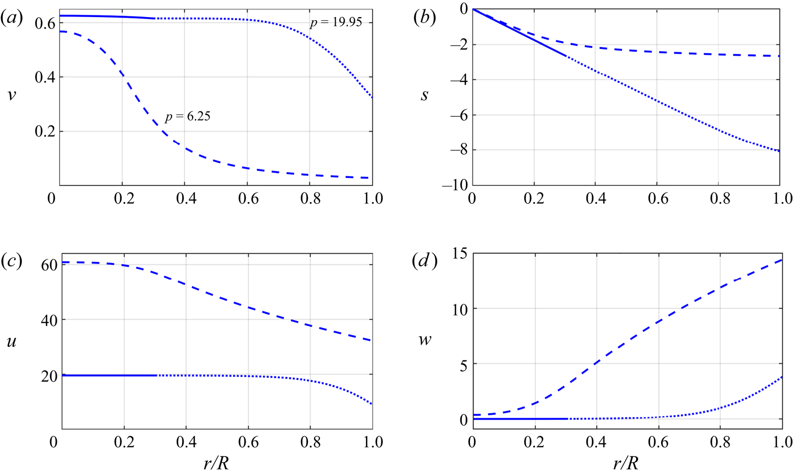
Figure 8. Profiles of (a)  $\nu$, (b) $s$, (c) $u$, and (d) $w$, for $Q=150$ and $R=14$, on the low-pressure and high-pressure branches. The higher-pressure solutions include an erodible bed that is indicated by the solid lines.
In the results presented thus far, the coefficient of normal restitution  $e_n$ has been taken as $0.85$. In figure 9, we show the effect of the coefficient of normal restitution $e_n$ on the variation of pressure with total mass flow rate. Lower coefficients of restitution lead to increased dissipation of kinetic energy and consequently granular temperature. Therefore, for a fixed mass flow rate, the pressure in the chute decreases when the coefficient of restitution is reduced. In Appendices A and B we present the effect of the dimensionless stiffness and critical solid volume fraction on the flow behaviour.
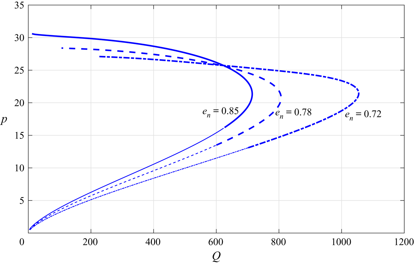
Figure 9. Variation of pressure  $p$ with the total flow rate $Q$, for chute width $R=20$ and three values of $e_n$. The thick lines indicate collisional flows with a bed; the thin lines indicate the collisional flows without a bed.
Vescovi et al. (Reference Vescovi, Berzi, Richard and Brodu2014) have shown that for coefficients of restitution within the range 0.7–0.95, the EKT predictions of granular temperature and stresses, for plane shear flows of frictionless spheres, are well within the numerical simulation results in the entire range of volume fractions. Berzi & Jenkins (Reference Berzi and Jenkins2018) compared the predictions of theories that are linear and nonlinear in the spatial gradients with the results of numerical simulations of steady, homogeneous shearing at a normal coefficient of restitution  $0.70$. The results indicate that the theory linear in the spatial gradients is performing rather well in this simple flow. In the next subsection, we compare our predictions using EKT with the DEM simulation results of Debnath et al. (Reference Debnath, Kumaran and Rao2022a).
5.1. Comparison with DEM results
In this subsection, we compare our results with the DEM simulation results of Debnath et al. (Reference Debnath, Kumaran and Rao2022a) for  $R=20$. In order to do this, we calculate the volume flow rate via numerical integration from the profiles of solid volume fraction $\nu$ and mean velocity $u$ across the half chute width obtained from DEM simulations for a specified average solid volume fraction $(\bar {\phi })$. For the parameter values $\mu = 0.5$, $e_n = 0.7$, $k_n = 1.2 \times 10^6$ and $R= 20$, and the flow rate $Q$, and compare the profiles $\nu$ and $u$ with those of Debnath et al. (Reference Debnath, Kumaran and Rao2022a). As shown in figure 10, the results are in good agreement. This is quite remarkable, considering that the normal coefficient of restitution is 0.7. The flow rates at $\bar {\phi }=0.61$, 0.60 and $0.59$, and chute width $R=20$, calculated from Debnath et al. (Reference Debnath, Kumaran and Rao2022a), are $65$,
$65$,  $105$ and $147$, respectively. For the same flow rates, the average solid volume fractions $\bar {\nu }_{total}$ across the same half chute width predicted by EKT are $0.616$, $0.612$ and $0.608$, respectively. In the limit $\nu \to \nu _c$, the slope of $\nu$ in the collisional regime approaches zero. This was also shown by Debnath et al. (Reference Debnath, Kumaran and Rao2022a). It can also be shown that the slope of $\nu$ in the bed at the interface is small, negative and independent of $\nu _c$. Therefore, there is a discontinuity in the slope of $\nu$ at the interface, which leads to the kink at the interface in the profile of $\nu$ obtained from EKT, as shown in figures 10(d–f).
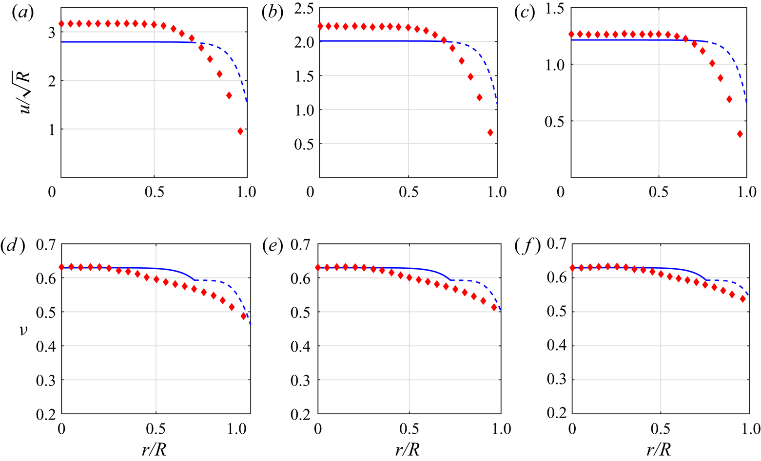
Figure 10. Profiles of (a–c)  $u/\sqrt {R}$, and (d–f) $\nu$. The DEM results of Debnath et al. (Reference Debnath, Kumaran and Rao2022a) correspond to symbols, and the blue curves correspond to the results predicted by EKT. The erodible bed is indicated by the solid lines. All the profiles are for the half chute width $R=20$: (a,d) $\bar {\phi }=0.59$, $Q=147$, $\bar {\nu }_{total}=0.608$; (b,e) $\bar {\phi }=0.60$, $Q=105$, $\bar {\nu }_{total}=0.612$; (c,f) $\bar {\phi }=0.614$, $Q=65$, $\bar {\nu }_{total}=0.616$; where $\bar {\phi }$ and $Q$ are from Debnath et al. (Reference Debnath, Kumaran and Rao2022a), corresponding to the $\bar {\nu }_{total}$ predictions of EKT.
In figure 11, we present the comparison of shear stress profile across the half chute width for  $R=15$ (figure 11a) and $R=20$ (figure 11b) with $\bar {\phi }= 0.60$ from Debnath et al. (Reference Debnath, Kumaran and Rao2022a), which corresponds to $\bar {\nu }_{total}=0.612$ in the EKT predictions. We find that the variations of shear stress across the chute are in good agreement with the measurements of Debnath et al. (Reference Debnath, Kumaran and Rao2022a). In the insets of figures 11(a) and 11(b), we also present the variation of dynamic friction coefficient $-s/p$ across the half chute width for $R=15$ and $20$ . However, the pressure is constant across the chute and $s/p$ is just a scaled representation of the shear stress for the vertical chute. (The solid volume fraction $\nu$ is continuous at the interface (i.e. $\nu =\nu _c$); however, the radial distribution function $g_0$ is singular at $\nu =\nu _c$. To avoid this singularity, we take the interface condition to be $\nu =\nu _c - \varepsilon$, where $\varepsilon$ is small. This numerical artefact leads to a jump in pressure from the erodible bed to the collisional flow; this jump decreases with $\varepsilon$.) In contrast, in the inclined flow, the pressure and shear stress both vary with the depth of the bed, and the dynamic friction coefficient is an important parameter there.
Figure 11. Profiles of  $-s/R$ for (a) $R=15$ and (b) $R=20$. The DEM results of Debnath et al. (Reference Debnath, Kumaran and Rao2022a) correspond to symbols, and the blue curves correspond to the results predicted by EKT. The erodible bed is indicated by the solid lines. Profiles are at $\bar {\phi }=0.60$, $Q=105$ from Debnath et al. (Reference Debnath, Kumaran and Rao2022a), which correspond to the predictions of EKT at $\bar {\nu }_{total}=0.6119$, $Q=105$. (c) Variation of scaled pressure $p/R$ with average solid volume fraction $\bar {\nu }_{total}$. (d) Variation of collisional flow width $h_1$, corresponding to the thickness of shear layer variation from Debnath et al. (Reference Debnath, Kumaran and Rao2022a) with $\bar {\nu }_{total}$. In (c) and (d). $R=15$ and $R=20$ are given by triangles and diamonds, respectively. The insets in (a) and (b) show variation of the dynamic friction coefficient $-s/p$ across the half chute width at the same parameter values of (a) and (b), respectively.
Further, in figure 11(c), we report the variation of scaled pressure with average solid volume fraction for  $R=15$ and $20$, compared with that reported by Debnath et al. (Reference Debnath, Kumaran and Rao2022a). The EKT results are closer to the DEM simulation predictions than the predictions of other theories considered by Debnath et al. (Reference Debnath, Kumaran and Rao2022a) (not shown). As reported in Debnath et al. (Reference Debnath, Kumaran and Rao2022a), we also observe that for a specified $R$, pressure $p$ decreases as average solid volume fraction $\bar {\nu }_{total}$ decreases. In figure 11(d), the variation of the thickness of the shear layer with average solid volume fraction in Debnath et al. (Reference Debnath, Kumaran and Rao2022a) is compared with the variation of the collisional flow width ( $h_1$) with $\bar {\nu }_{total}$. Again, the variation of the collisional flow width with the average solid volume fraction matches quite well with the corresponding shear layer thickness variation in Debnath et al. (Reference Debnath, Kumaran and Rao2022a), compared to the prediction of the other theories considered there (not shown).
6. Conclusions
We have employed extended kinetic theory to study steady, fully developed flows of deformable, inelastic, spherical grains driven by gravity between identical bumpy walls. For a given chute width and total flow rate, there exist two solutions characterized by high and low pressures. The solution with the higher pressure is denser and has a smaller mean velocity than the solution with the lower pressure. Also, for a range of the total flow rate, the solution branch at the higher pressure has a solid volume fraction near the centreline that is large enough to form an erodible bed. We also compared the profiles of the mean velocity, solid volume fraction and shear stress for the scenario with erodible bed obtained from the EKT and the DEM simulation of Debnath et al. (Reference Debnath, Kumaran and Rao2022a) for a few sets of parameters, and obtained excellent agreement. We will address the stability of the two solution branches in subsequent work.
Declaration of interests
The authors report no conflict of interest.
Appendix A. Effect of dimensionless stiffness ( $k_n$)

In this appendix, we study the effect of dimensionless stiffness on the flow behaviour. We vary the dimensionless stiffness  $k_n$ from $3\times 10^{6}$ to $3\times 10^{14}$. The other parameters are $\mu =0.15$, $e_n=0.85$ and $R=20$. Figures 12(a,b) show the variation of average solid volume fraction and average velocity, respectively with the volume flow rate. Considerable variation is observed above the dimensionless stiffness value $3\times 10^{8}$. The effect of stiffness on the variation of pressure with the volume flow rate is less (figure 12c), whereas the collisional flow width changes significantly with the stiffness (figure 12d).
Figure 12. Variation with the total flow rate  $Q$ of (a) average solid fraction, (b) average velocity, (c) wall pressure and (d) collisional flow width, for chute width $R=20$ for different values of dimensionless stiffness $k_n$. The thick lines indicate collisional flows with a bed; the thin lines indicate the collisional flows without a bed.
We also present the profiles of  $\nu$, $s$,
$s$,  $u$ and $w$ on the low-pressure and high-pressure branches for the different values of dimensionless stiffness as shown in figure 13. Recently, Debnath, Rao & Kumaran (Reference Debnath, Rao and Kumaran2022b) have shown that the effect on the temperature of the stiffness variation is less in the collisional flow and higher in the bed. With an increase in stiffness, the temperature decreases in the bed. They also report that the profiles of solid volume fraction and velocity above $k_n\geq 10^5$ are independent of $k_n$. We also found that variations in stiffness above $3 \times 10^6$ have little effect on the variation of solid volume fraction, shear stress and velocity in the collisional region, but do effect the bed.
Figure 13. Profiles of (a)  $\nu$, (b) $s$, (c) $u$, and (d) $w$, for $Q=600$ and $R=20$, on the low-pressure and high-pressure branches. The higher-pressure solutions include an erodible bed that is indicated in different colours. The black dotted line corresponds to $k_n=3\times 10^{12}$, the red dashed line corresponds to $k_n=3\times 10^{8}$, and the green line corresponds to $k_n=3\times 10^{6}$. The thinner lines correspond to the lower-pressure solutions and do not change much while changing the stiffness values. The inset in (d) is the variation of temperature across the chute for $R=20$, where the blue line, green line, red line and black line correspond to the $k_n$ values $3\times 10^{6}$, $3\times 10^{7}$, $3\times 10^{8}$ and $3\times 10^{12}$, respectively.
We found that there is an increase in the width of the erodible bed with the stiffness  $k_n$ between $3 \times 10^8$ and $3 \times 10^{12}$. The EKT prediction of temperature profiles across the chute at different stiffness values is shown in the inset of figure 13(d); it agrees qualitatively with the observation of Debnath et al. (Reference Debnath, Rao and Kumaran2022b) (not shown) that it decreases with increasing stiffness. Also, Debnath et al. (Reference Debnath, Rao and Kumaran2022b) claim that the decrease in granular temperature due to increase in stiffness suggests that $T$ will decrease to zero in the hard particle limit; the same is reflected by EKT predictions as the temperature is close to zero at stiffness value $3\times 10^{12}$.
Appendix B. Effect of the critical solid volume fraction ($\nu _c$)

The critical solid volume fraction and its dependence on the particle friction coefficient has been discussed in detail by Chialvo et al. (Reference Chialvo, Sun and Sundaresan2012). In order to change the value of  $\nu _c$, we must change the value of friction coefficient $\mu$. The other parameters used are $e_n=0.7$ and $k_n=3 \times 10^6$, unless specified otherwise. For the $\mu$ values $0.1105$, $0.32$ and $0.5$, the corresponding profiles of velocity and solid volume fraction for $R=20$ at different flow rates, and that from Debnath et al. (Reference Debnath, Kumaran and Rao2022a), are shown in figure 14. As we increase $\mu$, $\nu _c$ and the average solid volume fraction increase, and at the same volume flow rates, the corresponding profiles show small quantitative changes. Decrease of the particle friction coefficient decreases the thickness of the erodible bed and increases that of the collisional flow. Also with decrease of the particle friction coefficient, the velocity profiles decrease in the erodible bed region, and the solid volume fraction increases. These profiles do not vary much with $\mu$ (or $\nu _c$) near the bumpy boundary.
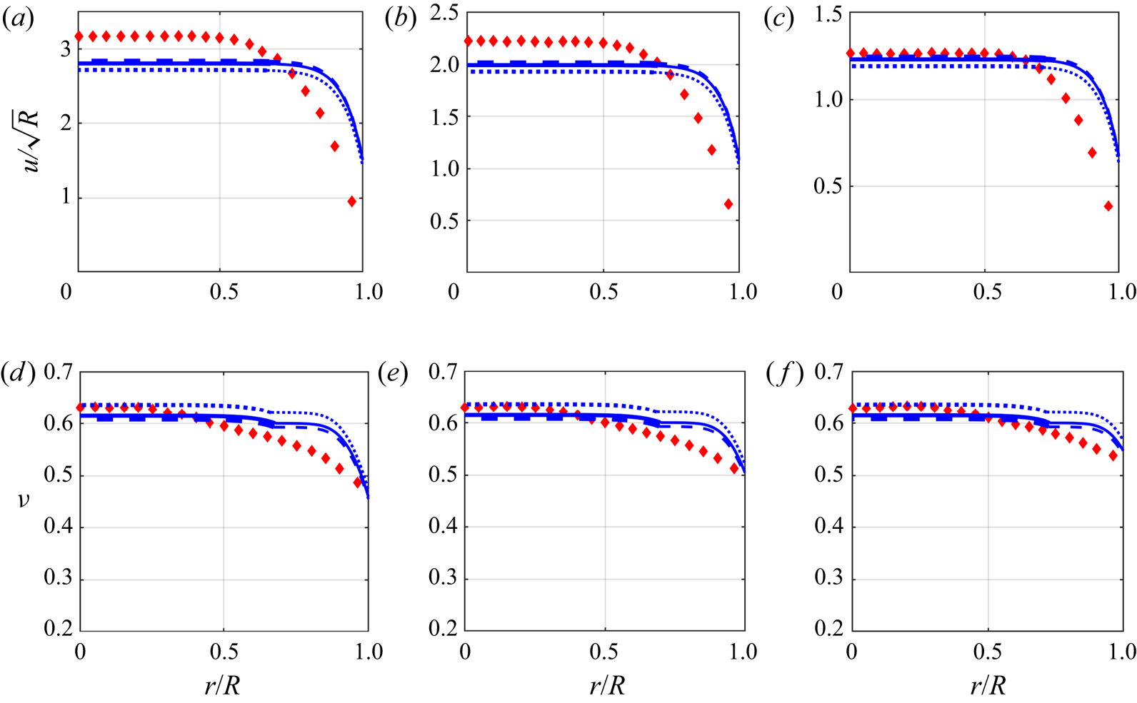
Figure 14. Profiles of (a–c)  $u / \sqrt {R}$, and (d–f) $\nu$. The DEM results of Debnath et al. (Reference Debnath, Kumaran and Rao2022a) correspond to symbols, and the blue curves correspond to the results predicted by EKT. The erodible bed is indicated by thicker blue lines. All the profiles are for the half chute width $R=20$: (a,d) $\bar {\phi }=0.59$, $Q=147$; (b,e) $\bar {\phi }=0.60$, $Q=105$; (c,f) $\bar {\phi }=0.61$, $Q=65$; from Debnath et al. (Reference Debnath, Kumaran and Rao2022a), corresponding to the predictions of EKT. Dashed lines are at $\mu =0.5$ and $\nu _c=0.5929$; solid lines are at $\mu =0.32$ and $\nu _c=0.6001$; and dotted lines are at $\mu =0.1105$ and $\nu _c=0.6211$. The other parameters used are $k_n=3\times 10^6$ and $e_n=0.7$.
Figures 15(a,b) show the profiles of scaled shear stress across the half chute width for different critical solid volume fractions. There is little variation in erodible bed thickness and almost negligible change in the shear stress profiles. In figures 15(c,d), the profiles of scaled pressure and collisional flow width at different critical solid volume fractions are compared with the scaled pressure and shear layer thickness of Debnath et al. (Reference Debnath, Kumaran and Rao2022a). The results follow a similar trend with the average solid volume fraction as observed in Debnath et al. (Reference Debnath, Kumaran and Rao2022a).
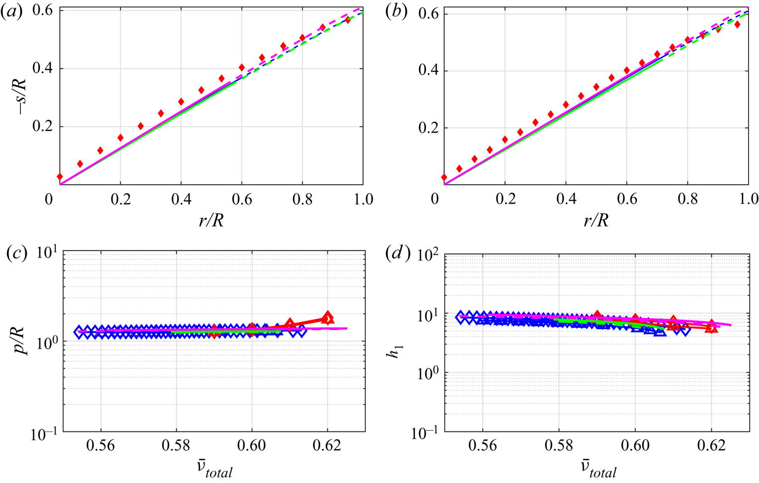
Figure 15. Profiles of  $-s/R$ for (a) $R=15$, and (b) $R=20$. The DEM results of Debnath et al. (Reference Debnath, Kumaran and Rao2022a) correspond to symbols, and the coloured lines correspond to the results predicted by EKT at different particle friction coefficients. The erodible bed is indicated by the solid lines. Profiles are at $\bar {\phi }=0.60$, $Q=105$ from Debnath et al. (Reference Debnath, Kumaran and Rao2022a), which correspond to the predictions of EKT at $Q=105$. Green lines are for $\mu =0.32$, $\nu _c=0.6003$ and $k_n=3 \times 10^6$; magenta lines are for $\mu =0.1105$, $\nu _c= 0.6211$ and $k_n=3 \times 10^6$; and blue lines are for $\mu =0.5$, $\nu _c=0.5929$ and $k_n=1.2\times 10^6$. (c) Variation of scaled pressure $p/R$ with average solid volume fraction $\bar {\nu }_{total}$. (d) Variation of collisional flow width $h_1$, corresponding to the thickness of shear layer variation from Debnath et al. (Reference Debnath, Kumaran and Rao2022a) with $\bar {\nu }_{total}$. In (c) and (d), $R=15$ and $R=20$ are represented by triangles and diamonds, respectively, for $\mu =0.5$, $\nu _c=0.592$ and $k_n=1.2 \times 10^6$. The green dashed lines and solid lines correspond to $\mu =0.32$, $\nu _c=0.6001$ and $k_n=3\times 10^6$ for $R=15$ and $R=20$, respectively. The magenta dashed lines and solid lines correspond to $\mu =0.1105$, $\nu _c=0.6211$ and $k_n=3\times 10^6$ for $R=15$ and $R=20$, respectively. The value of $e_n$ is taken as $0.7$ for all the profiles.


 Open access