3.1. Axisymmetric inertial-like waves

In this paper, we assume tacitly the existence of an axis of anisotropy in the $z$-direction, established by a secondary mechanism such as a magnetic field or rotation, to which, however, we make no reference. Consider an inviscid liquid endowed with odd viscosity as in (2.3), and an axially symmetric wave propagating along the axis of the magnetic field. Following Landau & Lifshitz (Reference Landau and Lifshitz1987, § 14), we consider cylindrical polar coordinates $r, \phi, z$ (cf. figure 2); the fields are independent of $\phi$, we neglect nonlinear terms (assuming small-amplitude motions), and the time and axial dependence are given by the factor $\exp [ {\rm i} (kz-\omega t)]$ where the frequency $\omega$ and wavenumber $k$ along the axis are both real. Employing the constitutive law (2.3), the linearized equations of motion (see Appendix A) become

(3.1)$$\begin{gather} -{\rm i}\omega v_r ={-}\frac{1}{\rho}\,\frac{\partial p'}{\partial r} - \nu_o\left[ \frac{1}{r}\, \frac{\partial}{\partial r} \left( r\,\frac{\partial v_\phi}{\partial r}\right) - \frac{v_\phi}{r^2}\right], \end{gather}$$

(3.2)$$\begin{gather}-{\rm i}\omega v_\phi = \nu_o\left[ \frac{1}{r}\,\frac{\partial}{\partial r} \left( r\,\frac{\partial v_r}{\partial r}\right) - \frac{v_r}{r^2}\right], \end{gather}$$

(3.3)$$\begin{gather}-{\rm i}\omega v_z ={-}\frac{{\rm i} k}{\rho}\,p', \end{gather}$$

where $p'$ is the variable part of the pressure in the wave, and $\rho$ is the liquid's constant density. The equation of continuity is

(3.4)\begin{equation} \frac{1}{r}\,\frac{\partial}{\partial r} \left( r v_r\right) + {\rm i} kv_z= 0. \end{equation}

Because of (3.3) and continuity,

(3.5)\begin{equation} p'/\rho = \omega v_z /k = \frac{{\rm i}\omega}{k^2}\,\frac{1}{r}\,\frac{\partial}{\partial r} ( r v_r), \end{equation}

and the identity

(3.6)\begin{equation} \frac{\partial}{\partial r} \left(\frac{1}{r}\,\frac{\partial}{\partial r} ( r v_r)\right) = \frac{1}{r}\, \frac{\partial}{\partial r} \left( r\,\frac{\partial v_r}{\partial r}\right) - \frac{v_r}{r^2}, \end{equation}

we obtain

(3.7)\begin{equation} \frac{1}{\rho}\,\frac{\partial p'}{\partial r} = \frac{{\rm i}\omega}{k^2} \left[ \frac{1}{r}\, \frac{\partial}{\partial r} \left( r\,\frac{\partial v_r}{\partial r}\right) - \frac{v_r}{r^2} \right]. \end{equation}

Thus, introducing the linear operator

(3.8)\begin{equation} \mathcal{L} = \partial_r^2 + \frac{1}{r}\,\partial _r - \frac{1}{r^2}, \end{equation}

the $r$ and $\phi$ momentum equations become

(3.9)$$\begin{gather} -{\rm i}\omega v_r ={-} {\rm i}\,\frac{\omega}{k^2}\,\mathcal{L} v_r - \nu_o\mathcal{L} v_\phi, \end{gather}$$

(3.10)$$\begin{gather}-{\rm i}\omega v_\phi = \nu_o\mathcal{L} v_r. \end{gather}$$

Expressing the velocities $v_r$ and $v_\phi$ in terms of Bessel or modified Bessel functions, $v_r = A\,{\rm J}_m(\kappa r)$, $v_\phi = B\,{\rm J}_m(\kappa r)$, or $v_r=A\,{\rm I}_m(\kappa r)$, $v_\phi =B\,{\rm I}_m(\kappa r)$, etc. (where $A$ and $B$ are constants, and $\kappa$ is an eigenvalue), we find that $m=1$. With the identity $\mathcal {L}\,{\rm J}_1(\kappa r) = - \kappa ^2\,{\rm J}_1(\kappa r)$, the system (3.9) and (3.10) has a solution when the determinant $\kappa ^4 k^2\nu _o^2 - \omega ^2(\kappa ^2 + k^2)$ of the coefficients of the resulting linear system

(3.11a,b)\begin{equation} Ak^2\omega - \kappa^2({\rm i}\nu_o Bk^2 - A\omega) =0 \quad \text{and} \quad {\rm i}\nu_o A\kappa^2 +\omega B = 0 \end{equation}

vanishes. Consider first the case where the origin is included in the domain. It is not difficult to show that the solution is the Bessel function ${\rm J}_1(\kappa r)$ for which $\kappa$ satisfies

(3.12)\begin{equation} \kappa^2 = \omega\,\frac{\omega \pm \sqrt{\omega^2 + (2k^2\nu_o)^2}}{2k^2\nu_o^2}. \end{equation}

Thus overall we found

(3.13a–c)\begin{align} v_r = A\,{\rm J}_1(\kappa r)\,{\rm e}^{{\rm i} (kz-\omega t)}, \quad v_\phi ={-}{\rm i}A\,\frac{\nu_o\kappa^2}{\omega}\,{\rm J}_1(\kappa r)\,{\rm e}^{{\rm i} (kz-\omega t)}, \quad v_z = {\rm i}A\,\frac{\kappa}{k}\,{\rm J}_0(\kappa r)\,{\rm e}^{{\rm i} (kz-\omega t)}. \end{align}

The motion comprises regions between coaxial cylinders with radius $r_n$ such that

(3.14)\begin{equation} r_n\kappa = \gamma_n, \end{equation}

and $\gamma _n$ are the zeros of ${\rm J}_1(x)$. Both $v_r$ and $v_\phi$ vanish at these coaxial cylinders, and the fluid does not cross them. The allowed values of the frequency $\omega$ in (3.12) are not restricted in any way in the infinite medium under consideration. (In contrast, in the rotating fluid case where $\kappa = k\sqrt {{4\varOmega ^2}/{\omega ^2} -1}$, the angular velocity $\varOmega$ of the liquid is required to satisfy the bound $\omega <2\varOmega$, for the solution to be finite.) In defining (3.12), we have assumed tacitly that the solutions that we pursue are finite in the radial direction $r$ and have thus discarded $\kappa$ terms associated with (exponentially increasing/decreasing) modified Bessel function solutions. The $\kappa$ terms in our discussion are always real (which can be justified by choosing large $\omega$, for instance).

Employing the radial and azimuthal momentum equations (3.1) and (3.2), we can now give a more satisfying explanation of the ‘elasticity’ of an odd viscous liquid and its tendency to restore a fluid particle back to its original position. Following Davidson (Reference Davidson2013, § 1.1) and Yih (Reference Yih1988, § 5), consider a circular ring of fluid in an odd viscous liquid with zero shear viscosity, located wholly on the $x$–$y$ plane. By some perturbation, the ring starts moving outwards with velocity $v_r>0$, and thus expands, so that $\partial _r v_r + ({1}/{r})v_r + ({1}/{r})\,\partial _\phi v_\phi >0$, where the last expression is the divergence of the velocity field in two dimensions. Rewrite (3.9)–(3.10) as

(3.15a,b)\begin{equation} -{\rm i}\omega \left(1 + \frac{\kappa^2}{k^2}\right) v_r= F_r, \quad -{\rm i}\omega v_\phi = F_\phi, \end{equation}

where $F_r \equiv - \nu _o\mathcal {L} v_\phi = \nu _o \kappa ^2 v_\phi$ and $F_\phi \equiv \nu _o\mathcal {L} v_r = -\nu _o\kappa ^2 v_r$. Since $v_r>0$, the second equation of (3.15) implies that there will be an azimuthal force $F_\phi = -\kappa ^2 \nu _o v_r<0$, an acceleration of the liquid in the $-\hat {\boldsymbol {\phi }}$ direction, and a commensurate negative velocity $v_\phi$, where we employed the eigenvalue $-\kappa ^2$ of the linear operator $\mathcal {L}$ in (3.8). This velocity will give rise to a radial force $F_r = - \kappa ^2 \nu _o\,|v_\phi |$ in the first equation of (3.15). This force endows the ring with an acceleration that points towards the origin, that is, towards the original location of the fluid ring, so it tries to reverse its expansion (the pressure contributes the $-{\rm i}\omega ({\kappa ^2}/{k^2})$ term in (3.15)). As the ring passes through its original position due to inertia and contracts, $\partial _r v_r + ({1}/{r})v_r + ({1}/{r})\,\partial _\phi v_\phi <0$, there will be a new azimuthal velocity component with sign opposite to the above one, that will lead to an eventual expansion towards equilibrium.

3.2. Axial inertial-like waves interior to a cylinder

We consider the liquid confined within a solid cylindrical surface located, say, at $r=a$, that would be realistic in a laboratory setting. This boundary will be a streamline located at an integral number of cells in the radial direction. If by $\gamma _n$ we denote the $n$th zero of the Bessel function ${\rm J}_1$, then (3.12) with the condition $\kappa a= \gamma _n$ leads to the constraint

(3.16)\begin{equation} a\left(\omega\,\frac{\omega + \sqrt{\omega^2 + (2k^2\nu_o)^2}}{2k^2\nu_o^2}\right)^{1/2} = \gamma_n, \end{equation}

and $n$ denotes the number of cells in the radial direction (cf. figure 3). From (3.16), we derive the dispersion relation

(3.17)\begin{equation} \omega = \frac{\nu_o k\gamma_n^2}{a \sqrt{k^2a^2 + \gamma_n^2}} , \end{equation}

where $n$ denotes the number of cells in the radial direction. (For clarity, we have suppressed the symbol $\pm$ in (3.17), and consider only the positive sign.) It is clear that in the limit $ka\gg \gamma _n$, the frequency in (3.17) becomes $\omega \sim {\nu _o}/{a^2}$, which recovers the qualitative frequency (1.4) that we obtained in the Introduction.

Figure 3. Instantaneous streamlines in the $r\unicode{x2013}z$ plane with streamfunction (3.18a–c), representing a simple harmonic wave propagating in the $z$-direction with phase velocity $c_p = \omega /k$ (see (3.19a,b)). Vertical lines are cross-sections of cylinders wrapping around the central axis, and were formed from the zeros of the Bessel function ${\rm J}_1$, where $v_r =0$. The radius $b$ of the external cylinder is determined by the condition $\kappa b = \gamma _3$, where $\gamma _3$ is the third root of the Bessel function ${\rm J}_1$ in the streamfunction (3.18a–c), or equivalently, in the radial velocity field in (3.13a–c).

In figure 3, we plot the streamlines interior to a cylinder of radius $b$ with the instantaneous streamfunction

(3.18a–c)\begin{equation} \psi(r,z) = \frac{\kappa}{3.83}\,r\,{\rm J}_1(\kappa r) \sin (kz), \quad v_z = \frac{1}{r}\,\frac{\partial \psi}{\partial r}, \quad v_r ={-}\frac{1}{r}\,\frac{\partial \psi}{\partial z}, \end{equation}

for $k=1$ and $\kappa = 2$ for comparison with figure 7.6.4 of Batchelor (Reference Batchelor1967, p. 561), which employs the same form for the streamfunction with the first zero $3.83$ of the Bessel function to modulate the amplitude in the denominator of (3.18a–c). The horizontal lines are locations where $v_r=0$ (zeros of the Bessel function).

There is important information to be surmised from the phase and group velocities

(3.19a,b)\begin{equation} c_p = \frac{\nu_o \gamma_n^2}{a \sqrt{k^2a^2 + \gamma_n^2}} \quad \text{and} \quad c_g =\frac{\nu_o \gamma_n^4}{a \left(k^2a^2 + \gamma_n^2\right)^{3/2}}, \end{equation}

that we derive from (3.17) (we have suppressed the symbol $\pm$ and employed only the positive sign in (3.17)). Since

(3.20)\begin{equation} c_p = c_g + \frac{a\nu_o k^2 \gamma_n^2}{ \left(k^2a^2 + \gamma_n^2\right)^{3/2}} > c_g, \end{equation}

the energy of a disturbance caused by a slowly moving body along the axis of the cylinder, with velocity $c_p$, cannot advance upstream relative to the body. Waves will be formed in the downstream direction. We reach the analogous conclusion if we employ the negative sign in (3.17). This situation is thus similar to the rotating liquid case, where the energy cannot propagate upstream and thus waves are formed only downstream, as described in many experiments, e.g. those of Long (Reference Long1953). We verify these claims in § 3.4 by combining numerical simulations of the Navier–Stokes equations with the theoretical predictions of the present subsection. (Note how the expression for $\omega$ in (3.17) contrasts with the inviscid liquid rotating at angular velocity $\varOmega$, where $\omega = 2\varOmega k/\sqrt {k^2 + ({\gamma _n}/{a})^2}$.)

3.3. Allowed wavenumbers

When the number of cells in the radial direction is $n$, from (3.16) allowed wavenumbers supporting propagation with phase velocity $c_p=\omega /k$, and for which the boundary at $r=a$ is a streamline, satisfy

(3.21)\begin{equation} ak = \gamma_n\left( \left(\frac{\nu_o\gamma_n}{ac_p}\right)^2 - 1\right)^{1/2}. \end{equation}

Wave propagation is thus possible when

(3.22)\begin{equation} \frac{ac_p}{\nu_o} < \gamma_n, \end{equation}

where $n$ denotes the number of cells in the radial direction. Thus although (3.12) does not introduce a restriction on frequencies for the propagation of waves, (3.21) does: defining a Maxworthy number $\mathcal {M}_a$ based on the phase velocity $c_p$ and cylinder radius $a$ (cf. (6.2a,b) for the definition of the dimensionless number $\mathcal {M}$),

(3.23)\begin{equation} \mathcal{M}_a = \frac{\nu_o}{ac_p}, \end{equation}

inertial motions with $n$ cylinders ($n$th zero of ${\rm J}_1$) are possible only when

(3.24)\begin{equation} \mathcal{M}_a > \frac{1}{\gamma_n}. \end{equation}

3.4. Numerical determination of odd viscous inertial oscillations inside a cylinder of radius $a$

By the inequality (3.20), we argued that, based on the inertial-like waves construction of §§ 3.1–3.3, the energy of a disturbance caused by a slowly moving body along the axis of the cylinder, with velocity $c_p$, cannot advance upstream relative to the body. Waves will be formed in the downstream direction.

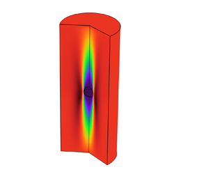
To verify this claim, we perform numerical simulations of the full Navier–Stokes equations of a slowly moving body with velocity $U=0.05\,{\rm cm}\,{\rm s}^{-1}$ in a cylinder of base radius $a = 25$ cm filled with an odd viscous liquid of dynamic coefficient $\eta _o = 0.7\,{\rm g}\,({\rm cm}\,{\rm s})^{-1}$, shear viscosity $\eta = 0.01\,{\rm g}\,({\rm cm}\,{\rm s})^{-1}$ and density $\rho = 1.1\,{\rm g}\,\text {cm}^{-3}$. Figure 4(b) displays the streamlines in the $r\unicode{x2013}z$ plane of the liquid downstream of the moving body, which show wave-like behaviour. To determine the wavelength, the colour bar shows the strength of the radial liquid velocity $v_r$ whose direction changes sign as we move down. From the plot, we can determine visually that the wavelength $\lambda$ is approximately $25$ cm. We compare this estimate to the theoretical prediction of §§ 3.1–3.3: from (3.21), we find that

(3.25)\begin{equation} \lambda = \frac{2{\rm \pi}}{k} = \frac{2{\rm \pi} a}{\gamma_1 \sqrt{\left(\dfrac{\nu_o \gamma_1}{aU}\right)^2 - 1}} =24.4764\,\text{cm}, \end{equation}

where $\gamma _1 = 3.8317$ is the first root of the Bessel function ${\rm J}_1$. Figure 4(a) displays the same system as in figure 4(b) but with $\eta_o =0$. No radial disturbance is visible in this case. Figure 4 was produced with the finite-element package comsol by solving the full Navier–Stokes equations in a three-dimensional axisymmetric domain. The flow Reynolds number, based on cylinder radius $a=25$ cm, is 125.

Figure 4. (a) In the absence of odd viscosity, no radial disturbance is visible as we move down and away from the body. The colour bar denotes radial velocity. The plot was produced with the finite-element package comsol by solving the full Navier–Stokes equations including inertial terms in a three-dimensional axisymmetric domain. (b) Waves generated by a small ($3.8$ cm) slowly-moving sphere (located at the centre of the cylinder – upper left of the plot) in an odd viscous liquid contained in a cylinder of radius $25$ cm. The colour bar denotes the strength of the radial liquid velocity $v_r$. Its direction changes sign as we move down and away from the body, and it is thus responsible for the distortion of the streamlines (in white). From this plot, we can determine visually the wavelength to be approximately $25$ cm. This agrees rather well with the theoretical estimate $24.476$ cm obtained from (3.25).

This situation is thus analogous to the rotating liquid case where the energy cannot propagate upstream and thus waves are formed only downstream, as described by the experiments of Long (Reference Long1953); cf. Batchelor (Reference Batchelor1967, pp. 564–566 and plate 24).

3.5. Axial inertial-like waves exterior to a cylinder

The above discussion can also be employed to establish wave propagation when the odd viscous liquid occupies the region $r>a$, exterior to a solid cylinder located at $r=a$. Now, the solution is of the form of a Bessel function of the second kind in the radial coordinate,

(3.26a–c)\begin{align} v_r = A\,{\rm Y}_1(\kappa r)\,{\rm e}^{{\rm i} (kz-\omega t)}, \quad v_\phi ={-}{\rm i}A\,\frac{\nu_o\kappa^2}{\omega}\,{\rm Y}_1(\kappa r)\,{\rm e}^{{\rm i} (kz-\omega t)}, \quad v_z = {\rm i}A\,\frac{\kappa}{k}\,{\rm Y}_0(\kappa r)\,{\rm e}^{{\rm i} (kz-\omega t)}, \end{align}

and the results of the previous subsections hold with the replacement

(3.27a,b)\begin{equation} {\rm J}_1 \rightarrow {\rm Y}_1, \quad \gamma_n \rightarrow \alpha_n, \end{equation}

where $\alpha _n$ is the $n$th zero of ${\rm Y}_1(x)$. In figure 5, we plot the streamlines exterior to a cylinder of radius $b$ with the instantaneous streamfunction

(3.28a–c)\begin{equation} \psi(r,z) = \frac{\kappa}{3.83}\,r\,{\rm Y}_1(\kappa r) \sin (kz), \quad v_z = \frac{1}{r}\,\frac{\partial \psi}{\partial r}, \quad v_r ={-}\frac{1}{r}\,\frac{\partial \psi}{\partial z}, \end{equation}

for $k=1$ and $\kappa = 2$ for comparison with figure 7.6.4 of Batchelor (Reference Batchelor1967, p. 561).

Figure 5. Instantaneous streamlines exterior to a cylinder of radius $r={\alpha _3}/{\kappa }$, where $\alpha _3$ is the third zero of ${\rm Y}_1$. This is a simple harmonic wave propagating in the $z$-direction with phase velocity $\omega /k$. Vertical lines correspond to zeros of the Bessel function of the second kind ${\rm Y}_1$, where $v_r =0$.

3.6. Plane-polarized waves induced by odd viscosity

The axisymmetric inertial-like waves that we discussed earlier propagate along the $z$ axis (the axis of anisotropy) and are three-dimensional in the sense that the wave amplitude varies along both the propagation direction and normal to it. In this subsection, we will consider different types of inertial-like waves that propagate along an arbitrary direction $\unicode{x1D4C0}$ and are polarized in the plane perpendicular to the propagation axis. This subsection follows the notation of Landau & Lifshitz (Reference Landau and Lifshitz1987, § 14). The odd-viscous Navier–Stokes equations

(3.29)\begin{equation} \frac{{\rm D}\boldsymbol{v}}{{\rm D}t} ={-}\frac{1}{\rho}\,\boldsymbol{\nabla} p +\nu_o\, \nabla_2^2\hat{\boldsymbol{z}} \times \boldsymbol{v}, \end{equation}

where $\nabla ^2_2 = \partial _x^2 + \partial _y^2$ and ${\rm D}/{\rm D}t$ is the convective derivative, become, after taking the curl of both sides,

(3.30)\begin{equation} \frac{{\rm D}}{{\rm D}t}\text{curl}\,\boldsymbol{v} =(\text{curl}\,\boldsymbol{v}) \boldsymbol{\cdot} \boldsymbol{\nabla} \boldsymbol{v} - \nu_o\,\nabla_2^2\,\frac{\partial \boldsymbol{v}}{\partial z}. \end{equation}

Linearizing,

(3.31)\begin{equation} \partial_t\,\text{curl}\,\boldsymbol{v} ={-} \nu_o\,\nabla_2^2 \frac{\partial \boldsymbol{v}}{\partial z}, \end{equation}

we seek plane-wave solutions of the form

(3.32)\begin{equation} \boldsymbol{v} = \boldsymbol{A} \exp({{\rm i}(\boldsymbol{k}\boldsymbol{\cdot} \boldsymbol{r} - \omega t)}), \end{equation}

where $\boldsymbol {A}$ is normal to $\boldsymbol {k}$ from the incompressibility condition.

Substituting the plane-wave solution into (3.31), we obtain

(3.33)\begin{equation} \omega \boldsymbol{k} \times \boldsymbol{v} = {\rm i} \nu_o (k_x^2 + k_y^2) k_z\boldsymbol{v}. \end{equation}

Taking the cross-product of both sides of (3.33) with $\boldsymbol {k}$, we obtain

(3.34)\begin{equation} {-\omega} k^2 \boldsymbol{v} = {\rm i} \nu_o (k_x^2 + k_y^2) k_z\boldsymbol{k} \times \boldsymbol{v}. \end{equation}

System (3.33)–(3.34) has a solution when the determinant of the coefficients vanishes. Solving for $\omega$, we obtain

(3.35)\begin{equation} \omega ={\pm} \frac{\nu_o (k_x^2 + k_y^2) k_z}{k}, \quad \text{or} \quad \omega ={\pm} \nu_o k^2 \cos\theta \sin^2\theta, \end{equation}

where $k = \sqrt {k_x^2 + k_y^2 + k_z^2}$, and the latter equation implies that $\theta$ is the angle between $\boldsymbol {k}$ and the anisotropy axis (cf. figure 6). In figure 7, we plot the dispersion $\omega$ (see (3.35)) versus angle $\theta$ between the wavevector $\boldsymbol {k}$ and the $z$ (anisotropy) axis. It differs qualitatively from the corresponding relation

(3.36)\begin{equation} \omega = 2\varOmega \cos \theta \end{equation}

of a (non-odd viscous) inviscid fluid rotating with angular velocity $\varOmega$; cf. Greenspan (Reference Greenspan1968). Comparing (3.35) with (3.36), when the coefficients $\nu _o$ and $\varOmega$ are kept constant, it becomes evident that the dispersion relation (3.35) obtained due to the specific form of the constitutive law (2.3) that we adopted for an odd viscous liquid becomes prominent for large in-plane wavenumbers and small corresponding wavelengths.

Figure 6. (a) Coordinate system employed in plane-polarized waves, showing the definition of angles for the propagation wavevector $\boldsymbol {k}$. (b) When the propagation direction is normal to the axis $\hat {\boldsymbol {z}}$, the group velocity $\boldsymbol {c}_g = \boldsymbol {\nabla }_{\boldsymbol {k}}\omega$ in (3.41) becomes co-axial to the axis $\hat {\boldsymbol {z}}$, and acquires its maximum value.

Figure 7. Subsection 3.6 plane-polarized wave dispersion $\omega$ (see (3.35)) versus angle $\theta$ between the wavevector $\boldsymbol {k}$ and the $z$ (anisotropy) axis (setting $k=\nu _o = 1$). Of interest is the low-frequency range at $\theta \sim {{\rm \pi} }/{2}$ where group velocity is maximum. This curve structure should be contrasted to the corresponding relation $\omega = 2\varOmega \cos \theta$ of an inviscid fluid rotating with angular velocity $\varOmega$.

Following Landau & Lifshitz (Reference Landau and Lifshitz1987), we introduce the unit vector $\hat {\boldsymbol {k}} = {\boldsymbol {k}}/{k}$ in the direction of the wavevector, and the complex amplitude $\boldsymbol {A} = \boldsymbol {a} +{\rm i} \boldsymbol {b}$, where $\boldsymbol {a}$ and $\boldsymbol {b}$ are real vectors. Considering (3.33) and the dispersion relation (3.35), we obtain $\hat {\boldsymbol {k}} \times \boldsymbol {b} = \boldsymbol {a}$, that is, the two vectors $\boldsymbol {a}$ and $\boldsymbol {b}$ are perpendicular to each other, are of the same magnitude, and lie in the plane whose normal is $\boldsymbol {k}$. Thus the velocity field is polarized circularly in the plane defined by $\boldsymbol {a}$ and $\boldsymbol {b}$, and is of the form

(3.37)\begin{equation} \boldsymbol{v} = \boldsymbol{a} \cos (\boldsymbol{k}\boldsymbol{\cdot} \boldsymbol{r} - \omega t) - \boldsymbol{b} \sin (\boldsymbol{k}\boldsymbol{\cdot} \boldsymbol{r} - \omega t), \quad \boldsymbol{a}\perp\boldsymbol{b}. \end{equation}

Employing the negative sign of the dispersion relation (3.35), the above analysis leads to the same velocity field (3.37) but with the sense of the vectors $\boldsymbol {a}$ and $\boldsymbol {b}$ reversed: $\hat {\boldsymbol {k}} \times \boldsymbol {b} = -\boldsymbol {a}$. This will become important in § 4, where the helicity associated with wave propagation will be determined.

It is of interest to calculate the direction of propagation of energy. We obtain

(3.38a–c)\begin{equation} \frac{\partial \omega}{\partial k_x} = \nu_o\,\frac{k_xk_z(k^2 + k_z^2)}{k^3}, \quad \frac{\partial \omega}{\partial k_y} = \nu_o\,\frac{k_yk_z(k^2 + k_z^2)}{k^3}, \quad \frac{\partial \omega}{\partial k_z} = \nu_o\,\frac{(k_x^2 + k_y^2)^2}{k^3}, \end{equation}

or, taking the $z$ axis to be the axis of anisotropy,

(3.39a,b)\begin{equation} \left(\frac{\partial \omega}{\partial k_x}, \frac{\partial \omega}{\partial k_y} \right) = k\nu_o \sin \theta \cos \theta (1 + \cos^2 \theta)( \cos \phi, \sin \phi), \quad \frac{\partial \omega}{\partial k_z} = k\nu_o \sin^4 \theta. \end{equation}

The group velocity $\boldsymbol {c}_g = {\partial \omega }/{\partial \boldsymbol {k}}$ in vector form can be written as

(3.40)\begin{equation} \frac{\partial \omega}{\partial \boldsymbol{k}} = \nu_ok \left\{ \hat{\boldsymbol{k}}(\hat{\boldsymbol{z}}\boldsymbol{\cdot} \hat{\boldsymbol{k}}) \left[ 1+ (\hat{\boldsymbol{z}}\boldsymbol{\cdot} \hat{\boldsymbol{k}})^2\right] + \hat{\boldsymbol{z}}\left[1- 3(\hat{\boldsymbol{z}}\boldsymbol{\cdot} \hat{\boldsymbol{k}})^2 \right] \right\}, \end{equation}

which can be compared with its rigidly rotating (non-odd viscous) counterpart ${\partial \omega }/{\partial \boldsymbol {k}} = ({2\varOmega }/{k})[\hat {\boldsymbol {z}} - \hat {\boldsymbol {k}}(\hat {\boldsymbol {z}}\boldsymbol {\cdot } \hat {\boldsymbol {k}}) ]$, where the group velocity is perpendicular to the phase velocity $\boldsymbol {c}_p = ({\omega }/{k}) \hat {\boldsymbol {k}}$ (see table 1). Here, the group velocity is not perpendicular to the phase velocity. A calculation gives $\boldsymbol {c}_g \boldsymbol {\cdot } \boldsymbol {c}_p = 2|\boldsymbol {c}_p|^2 = 2\nu _o^2k^2\cos ^2\theta \sin ^4\theta$. Thus, in contrast to the case of inertial waves in a rotating fluid where the energy propagates perpendicularly to the wavevector, here the energy propagation direction has a component along the $\hat {\boldsymbol {k}}$ axis. The modulus of the group velocity is

(3.41)\begin{equation} \left|\frac{\partial \omega}{\partial \boldsymbol{k}} \right|= k\nu_o \sin\theta \sqrt{5 \cos^4\theta - 2 \cos^2 \theta + 1}. \end{equation}

In figure 8, we plot the group velocity components (3.39a,b) and its magnitude (3.41) versus angle $\theta$ between the wavevector $\boldsymbol {k}$ and the $z$ (anisotropy) axis (setting $k=\nu _o = 1$).

Table 1. Summary of odd viscous plane-polarized inertial-like wave behaviour at low and high frequencies (see (3.35)) and comparison with their rigidly rotating counterparts. Here, $\boldsymbol {c}_g$ is the group velocity ${\partial \omega }/{\partial \boldsymbol {k}}$, and $\boldsymbol {c}_p = ({\omega }/{k}) \hat {\boldsymbol {k}}$ is the phase velocity. The group velocity is maximum when the angle is $\theta = {\rm \pi}/2$, propagation takes place perpendicular to the anisotropy axis ($\hat {\boldsymbol {z}}$), the group velocity acquires its maximum propagation along the anisotropy axis, and helicity becomes segregated; cf. § 4. Helicity density $\boldsymbol {v} \boldsymbol {\cdot } \text {curl}\,\boldsymbol {v}$ has the same functional form in both odd viscous and rigidly rotating liquids. Although in a rigidly rotating liquid the group velocity is always perpendicular to the phase velocity, in an odd viscous liquid there is dependence on the angle $\theta$ (see the third row of the table), were $\theta$ denotes the angle between $\boldsymbol {\varOmega } = \varOmega \hat {\boldsymbol {z}}$ and the propagation direction $\boldsymbol {k}$; cf. figure 6.

Figure 8. Subsection 3.6 plane-polarized wave group velocity components and magnitude (3.39a,b) and (3.41) versus angle $\theta$ between the wavevector $\boldsymbol {k}$ and the $z$ (anisotropy) axis, setting $k=\nu _o = 1$ (and $\phi ={\rm \pi} /4$, for simplicity). Of interest is the low-frequency range at $\theta \sim {{\rm \pi} }/{2}$, where group velocity is maximum. The modulus of the group velocity should be contrasted to $|{\partial \omega }/{\partial \boldsymbol {k}} |= (2\varOmega /k) \sin \theta$ in the case of an inviscid rigidly rotating liquid with angular velocity $\varOmega$.

In addition to the information in table 1, the frequency is maximum at $\theta =\cos ^{-1}({\sqrt {3}}/{3}) \sim 0.3{\rm \pi}$, acquiring the value $\omega = \pm \nu _ok^2({2\sqrt {3}}/{9})$. The group velocity becomes $({4k\nu _o}/{9})(\sqrt {2} \cos \phi, \sqrt {2} \sin \phi, 1)$, and its modulus is $c_g = 4k\nu _o \sqrt {3}/9$. In addition, the group velocity has a local maximum at $\theta =\cos ^{-1}({\sqrt {15}}/{5}) \sim 0.22{\rm \pi}$. The frequency is $\omega = \pm \nu _ok^2({2\sqrt {15}}/{25})$, and the group velocity becomes $({4k\nu _o}/{25})(2\sqrt {6} \cos \phi, 2\sqrt {6} \sin \phi, 1)$, with modulus $c_g = 4k\nu _o / 5$. Comparison can be made of (3.41) with plane-polarized waves rotating rigidly (Landau & Lifshitz Reference Landau and Lifshitz1987, § 14), where $|{\partial \omega }/{\partial \boldsymbol {k}} |= (2\varOmega /k) \sin \theta$.

4.1. Conservation of helicity in plane-polarized waves of an odd viscous liquid

From the plane-polarized velocity field (3.37), we obtain $\text {curl}\,\boldsymbol {v} =-\boldsymbol {k}\times \boldsymbol {b} \cos (\boldsymbol {k}\boldsymbol {\cdot } \boldsymbol {r} - \omega t)$$-\boldsymbol {k}\times \boldsymbol {a} \sin (\boldsymbol {k}\boldsymbol {\cdot } \boldsymbol {r} - \omega t)$. The relation $\hat {\boldsymbol {k}} \times \boldsymbol {b} = \pm \boldsymbol {a}$ (where the $\pm$ symbol corresponds to the sign of the dispersion relation (3.35)) leads to $\text {curl}\,\boldsymbol {v} = \mp k\boldsymbol {v}$, thus

(4.2a,b)\begin{equation} \boldsymbol{v} \boldsymbol{\cdot} \text{curl}\,\boldsymbol{v} ={\mp} k\,|\boldsymbol{v}|^2 \quad \text{and} \quad \mathcal{H} = \int_V \boldsymbol{v} \boldsymbol{\cdot} \text{curl}\,\boldsymbol{v}\,{\rm d}V ={\mp} k\,|\boldsymbol{v}|^2\,V, \end{equation}

where $|\boldsymbol {v}|^2=|\boldsymbol {a}|^2 + |\boldsymbol {b}|^2$ is the constant magnitude of the velocity in (3.37), $V$ is the volume of the region under consideration, and $k = \sqrt {k_x^2 + k_y^2 + k_z^2}$. The negative sign in (4.2a,b) (corresponding to the positive sign in the dispersion relation (3.35)) is associated with particle paths following left-handed helices, and the positive sign is associated with right-handed helices. Energy propagates along a cone whose normal is the vector $\hat {\boldsymbol {k}}$ (cf. Davidson (Reference Davidson2013) for the case of a rigidly rotating liquid).

Inertial-like waves give rise to maximal helicity. This can be seen by substituting (4.2a,b) into the the Cauchy–Schwarz inequality $\mathcal {H}^2\leq \mathcal {E}\mathcal {W}$ expressed in terms of the helicity (4.1) and the energy and enstrophy integrals (Moffatt Reference Moffatt1969)

(4.3a,b)\begin{equation} \mathcal{E} = \int_V \boldsymbol{v}^2 \,{\rm d}V , \quad \mathcal{W} = \int_V (\text{curl}\,\boldsymbol{v})^2 \,{\rm d}V. \end{equation}

As shown by Moffatt (Reference Moffatt1970) for the case of rigidly rotating liquids, inertial waves exhibit a loss of reflection symmetry when the energy propagates parallel to the rotation axis (and the phase velocity is perpendicular to this axis). Davidson (Reference Davidson2013) associates each direction of propagation of energy with one of the signs of helicity in (4.2a,b): negative sign of helicity for energy propagating in the $+\hat {\boldsymbol {z}}$ direction, and positive sign of helicity for energy propagating in the $-\hat {\boldsymbol {z}}$ direction. This is called the ‘segregation of helicity’ and has found applications in problems of magnetohydrodynamics (Davidson Reference Davidson2013; Davidson & Ranjan Reference Davidson and Ranjan2018). The waves that correspond to this type of behaviour have low frequencies (the frequency $\omega$ in (3.35) is nearly zero). The consequence of this behaviour in an odd viscous liquid can be seen more easily by going back to the original equation of motion (3.29). Linearizing, and taking the limit $\omega \rightarrow 0$, amounts to dropping the time derivative. Then the equation of motion becomes (5.1a–c) of the next section, which makes the dynamics effectively two-dimensional (perpendicular to the anisotropy axis), leads to the Taylor–Proudman theorem, and gives rise to Taylor columns.

4.2. Helicity in axisymmetric inertial-like waves of an odd viscous liquid

It turns out that vorticity is also parallel to the velocity field for the inertial-like waves of § 3.1. This can be shown directly by taking the curl of the velocity field (3.13a–c) and solving in expression (3.12) for the frequency $\omega = {\nu _o k\kappa ^2}/{\sqrt {k^2 + \kappa ^2}}$. (In contrast to the previous section, $k$ here denotes the wavenumber $k_z$ along the axis; cf. § 3.1.) Alternatively, setting $A = a\,{\rm e}^{{\rm i}\theta }$ for real amplitude $a$ and phase $\theta$, we obtain

(4.4a,b)\begin{equation} v_r = a\,{\rm J}_1(\kappa r)\cos(kz-\omega t+\theta), \quad v_\phi = \frac{\nu_o \kappa^2}{\omega}\,a\,{\rm J}_1(\kappa r)\sin(kz-\omega t+\theta), \end{equation}

and $v_z = -({\kappa }/{k})a\,{\rm J}_0(\kappa r)\sin (kz-\omega t+\theta )$. In either case, the final result is

(4.5a,b)\begin{equation} \text{curl}\,\boldsymbol{v} ={\mp} \sqrt{k^2 + \kappa^2}\,\boldsymbol{v} \quad \text{and} \quad \boldsymbol{v} \boldsymbol{\cdot} \text{curl}\,\boldsymbol{v} ={\mp} \sqrt{k^2 + \kappa^2}\,|\boldsymbol{v}|^2. \end{equation}

When the liquid is contained in a solid cylinder of radius $b$, $\omega$ is replaced by (3.17) and $\kappa$ by $\gamma _n/b$, where $\gamma _n$ is the $n$th zero of ${\rm J}_1(x)$.

8.1. Plane-polarized waves

We define the linear operator

(8.2)\begin{equation} \mathcal{S} = (\nu_o-\nu_4)\,\nabla^2_2 + \nu_4\,\partial_z^2, \end{equation}

where $\nu _4 = \eta _4/\rho$, and $\nabla ^2_2 = \partial _x^2 + \partial _y^2$. To obtain an understanding of the effect of odd viscosity parameters on the type of solutions, we classify the operator $\mathcal {S}$ in (8.2) as follows (assume here that $\nu _4>0$):

1. (i) $\mathcal {S}$ is elliptic when $\nu _o>\nu _4$;

2. (ii) $\mathcal {S}$ is hyperbolic when $\nu _o<\nu _4$;

3. (iii) $\mathcal {S}$ is parabolic when $\nu _o=\nu _4$.

Here, we have assumed that $z$ plays the role of the time-like variable. This is the standard route followed in rigidly rotating liquids; see Whitham (Reference Whitham1974, § 12.6). With the notation $\zeta = \partial _x v - \partial _y u$ for the component of vorticity in the $z$-direction, and a modified pressure $\tilde {p} = p + \eta _4 \zeta$, the Navier–Stokes equations (3.29) are replaced by

(8.3)\begin{equation} \frac{{\rm D}\boldsymbol{v}}{{\rm D}t} ={-}\frac{1}{\rho}\,\boldsymbol{\nabla} \tilde{p} +\mathcal{S}\hat{\boldsymbol{z}} \times \boldsymbol{v}, \end{equation}

and the vorticity equation (3.31) by

(8.4)\begin{equation} \partial_t\,\text{curl}\,\boldsymbol{v} ={-} \mathcal{S}\,\frac{\partial \boldsymbol{v}}{\partial z}. \end{equation}

With $\boldsymbol {v} = \boldsymbol {A} \exp ({{\rm i}(\boldsymbol {k}\boldsymbol {\cdot } \boldsymbol {r} - \omega t)})$, the vorticity equation (8.4) becomes a system of three equations for the three unknown components of the amplitude $\boldsymbol {A}$. This system has a non-trivial solution when the determinant of the matrix

(8.5)\begin{equation} \left(\begin{array}{@{}ccc@{}} -{\rm i}k_z\,\mathcal{S}(\boldsymbol{k}) & \omega k_z & -\omega k_y\\ -\omega k_z & -{\rm i}k_z\,\mathcal{S}(\boldsymbol{k}) & \omega k_x\\ \omega k_y & -\omega k_x & -{\rm i}k_z\,\mathcal{S}(\boldsymbol{k}) \end{array} \right) \end{equation}

vanishes. Here,

(8.6)\begin{equation} \mathcal{S}(\boldsymbol{k}) ={-} (\nu_o - \nu_4) (k_x^2+k_y^2) - \nu_4 k_z^2. \end{equation}

The dispersion relation becomes

(8.7)\begin{equation} \omega ={\mp} \mathcal{S}(\boldsymbol{k})\,\frac{k_z}{k} \quad \text{or} \quad \omega ={\pm} \cos (\theta )\,k^{2} \left[\nu_o -\nu_4 -\left(\nu_o -2 \nu_4 \right)\cos^{2}\theta \right]. \end{equation}

Here and below, the reader can keep in mind the parabolic case $\nu _o=\nu _4$ and the elliptic case $\nu _o = 2\nu _4$ (parabolic and elliptic with respect to the operator $\mathcal {S}$ in (8.2)), which simplify all relations significantly and are to be discussed in what follows.

We display the dispersion (8.7) for $\nu _o = 0$ in figure 12(a), to be compared with figure 7. This dispersion relation is interesting as it crosses the $\omega =0$ axis at angle $\theta = {\rm \pi}/4$ (different to the ${\rm \pi} /2$ of rigidly rotating liquids or the $\eta _o$ of odd viscous liquid). Likewise, it has an inflection point at $\theta \neq {\rm \pi}/2$, which signals the presence of a maximum for the group velocity that differs from those of rigidly rotating liquids and the $\eta _o$ of odd viscous liquid. The group velocity (3.39a,b) is replaced by

(8.8)$$\begin{gather} \left(\frac{\partial \omega}{\partial k_x}, \frac{\partial \omega}{\partial k_y} \right) ={\pm} k \left((\nu_o -2 \nu_4 ) \cos^{2}\theta+\nu_o -\nu_4 \right)\sin \theta \cos \theta\,( \cos \phi, \sin \phi), \end{gather}$$

(8.9)$$\begin{gather}\frac{\partial \omega}{\partial k_z} ={\pm} k \left((\nu_o -2 \nu_4 ) \cos^{4}\theta +(-2 \nu_o +5 \nu_4 )\cos^{2}\theta+\nu_o -\nu_4 \right), \end{gather}$$

with modulus

(8.10)$$\begin{gather} |c_g| = k \left[{-}5 (\nu_o -2 \nu_4 )^{2} \cos^{6}\theta + (7\nu_o -16 \nu_4) (\nu_o -2 \nu_4 ) \cos^{4}\theta \right.\nonumber\\ \left. {}-3 (\nu_o -\nu_4 ) (\nu_o -3 \nu_4 ) \cos^{2}\theta+(\nu_o -\nu_4 )^{2}\right]^{1/2}. \end{gather}$$

Its components and modulus are displayed in figure 12(b) for the case $\nu _o =0$. The modulus of the group velocity displays a maximum at $\theta \neq {\rm \pi}/2$, as expected from the properties of the corresponding dispersion relation (8.7).

Figure 12. (a) Plane-polarized wave dispersion $\omega$ (see (8.7)) versus angle $\theta$ between the wavevector $\boldsymbol {k}$ and the $z$ (anisotropy) axis (setting $k=-\nu _4 = 1$, $\nu _o = 0$). It differs qualitatively from its $\eta _o \neq 0$ counterpart displayed in figure 7 (and here denoted by the dash-dotted curve) by crossing the $\omega =0$ axis at angles different from ${\rm \pi} /2$. The case $\eta _0=2\eta _4$, discussed in detail in § 8.3, is denoted by the dashed curve. (b) Group velocity magnitude versus angle $\theta$ between the wavevector $\boldsymbol {k}$ and the $z$ (anisotropy) axis, setting $k=-\nu _4 = 1$, $\nu _o = 0$. The magnitude develops maxima at angles $\theta \neq {\rm \pi}/2$, differing from those of the rigidly rotating liquid or the $\eta _o$ odd viscous liquid (here denoted by the dash-dotted curve); cf. figure 8. The case $\eta _0=2\eta _4$, discussed in detail in § 8.3, is denoted by the dashed curve.

When the flow field is determined by the plane-polarized waves $\boldsymbol {v} = \boldsymbol {A} \exp ({{\rm i}(\boldsymbol {k}\boldsymbol {\cdot } \boldsymbol {r} - \omega t)})$ considered in this section, its helicity is conserved for an odd viscous liquid that incorporates both constitutive laws (7.1) and (8.1). That is the case because in wavenumber and frequency space, the linearized vorticity equation (8.4) can be written in the form

(8.11)\begin{equation} -{\rm i}\omega \boldsymbol{B} ={-} {\rm i} \boldsymbol{A}k_z\,\mathcal{S}(\boldsymbol{k}), \end{equation}

when $\text {curl}\,\boldsymbol {v} = \boldsymbol {B} \exp ({{\rm i}(\boldsymbol {k}\boldsymbol {\cdot } \boldsymbol {r} - \omega t)})$ and $\mathcal {S}(\boldsymbol {k})$ is defined in (8.6). Since $\omega = \mp \mathcal {S}(\boldsymbol {k})\,({k_z}/{k})$ (from (8.7)), we obtain $\boldsymbol {B} = \mp k \boldsymbol {A}$, or

(8.12)\begin{equation} \text{curl}\,\boldsymbol{v} ={\mp} k\boldsymbol{v}. \end{equation}

Thus the helicity of the flow field determined by the odd stress tensors (7.1) and (8.1) is conserved:

(8.13)\begin{equation} \boldsymbol{v} \boldsymbol{\cdot} \text{curl}\,\boldsymbol{v} ={\mp} k\,|\boldsymbol{v}|^2. \end{equation}

In addition, $\boldsymbol {c}_g \boldsymbol {\cdot } \boldsymbol {c}_p = 2 [ (\nu _o-2\nu _4)\cos ^2\theta -\nu _o+\nu _4 ]^2k^2\cos ^2\theta = 2\,|\boldsymbol {c}_p|^2$, so the last two rows of table 1 remain unchanged.

Equation (8.3) can be employed to investigate the possibility of Taylor column formation in an odd viscous liquid that incorporates the stress tensor (7.1) and (8.1). Dropping the left-hand side of (8.3), it reads, in component form,

(8.14a–c)\begin{equation} \frac{1}{\rho}\,\frac{\partial \tilde{p}}{\partial x} ={-}\mathcal{S} v, \quad \frac{1}{\rho}\,\frac{\partial \tilde{p}}{\partial y} = \mathcal{S} u, \quad \frac{\partial \tilde{p}}{\partial z} = 0, \end{equation}

and carrying out the same manipulations as in § 5, we obtain the conditions

(8.15a,b)\begin{equation} \partial_z\mathcal{S} u = \partial_z\mathcal{S}v=\partial_z\mathcal{S}w =0 \quad \text{and} \quad \partial_x\mathcal{S}u +\partial_y\mathcal{S} v =0, \end{equation}

which replace (5.7). The forms of equations (8.14a–c) and (8.15a,b) are appealing and resemble (5.1a–c) and (5.7), respectively. They still lead to Taylor-column-like structures, which, however, are not identical to those of rigidly rotating liquids.

8.2. Axisymmetric inertial-like waves when $\eta _o, \eta _4 \neq 0$

We express the constitutive law (8.1) in cylindrical coordinates as

(8.16)\begin{equation} \boldsymbol{\sigma}' = \eta_4 \left(\begin{array}{@{}ccc@{}} 0 & 0 & -\left(\dfrac{1}{r}\,\partial_\phi v_z + \partial_z v_\phi\right)\\ 0 & 0 & \partial_r v_z + \partial_z v_r\\ -\left(\dfrac{1}{r}\,\partial_\phi v_z + \partial_z v_\phi\right) & \partial_r v_z + \partial_z v_r & 0 \end{array} \right), \end{equation}

and repeat the construction of axial waves of § 3.4. The linearized equations of motion (see Appendix A) become

(8.17)$$\begin{gather} -{\rm i}\omega v_r ={-}\frac{1}{\rho}\,\frac{\partial p'}{\partial r} - (\nu_o-\nu_4)\left[ \frac{1}{r}\,\frac{\partial}{\partial r} \left( r\,\frac{\partial v_\phi}{\partial r}\right) - \frac{v_\phi}{r^2}\right] + \nu_4 k^2 v_\phi, \end{gather}$$

(8.18)$$\begin{gather}-{\rm i}\omega v_\phi = (\nu_o-\nu_4)\left[ \frac{1}{r}\,\frac{\partial}{\partial r} \left( r\, \frac{\partial v_r}{\partial r}\right) - \frac{v_r}{r^2}\right] - \nu_4 k^2 v_r , \end{gather}$$

(8.19)$$\begin{gather}-{\rm i}\omega v_z ={-}\frac{{\rm i} k}{\rho}\,p' - {\rm i}k \nu_4\,\frac{1}{r}\,\frac{\partial}{\partial r}(r v_\phi) , \end{gather}$$

where we simplified (8.18) by employing the incompressibility condition (3.4). Introducing the linear operator (3.8) $\mathcal {L} = \partial _r^2 + ({1}/{r})\,\partial _r - 1/r^2$, the $r$ and $\phi$ momentum equations become

(8.20)$$\begin{gather} -{\rm i}\omega v_r ={-} {\rm i}\,\frac{\omega}{k^2}\,\mathcal{L} v_r +\nu_4(\mathcal{L} +k^2) v_\phi-\nu_o\mathcal{L}v_\phi, \end{gather}$$

(8.21)$$\begin{gather}-{\rm i}\omega v_\phi ={-}\nu_4(\mathcal{L} +k^2) v_r + \nu_o\mathcal{L}v_r. \end{gather}$$

System (8.20)–(8.21) has a solution when the determinant $-(\nu _o -\nu _4 )^{2} k^{2} \kappa ^{4}+(-2 k^{4} \nu _o \nu _4 +2 k^{4} \nu _4^{2}+\omega ^{2}) \kappa ^{2}-k^{2} (k^{2} \nu _4 -\omega ) (k^{2} \nu _4 +\omega )$ of the coefficients of the resulting linear system

(8.22a,b)\begin{align} &\frac{{\rm i}Bk^{4} \nu_4 \,{+}\,{\rm i} (\nu_o \,{-}\,\nu_4 ) \kappa^{2} B k^{2}\,{-}\,A \,\kappa^{2} \omega}{k^{2} \omega}-A =0\quad \text{and}\quad -\frac{{\rm i} A \left((\nu_o \,{-}\,\nu_4 ) \kappa^{2}\,{+}\,k^{2} \nu_4 \right)}{\omega}\,{-}\,B = 0 \end{align}

vanishes.

The velocity field is again expressed with respect to Bessel functions: $v_r = A\,{\rm J}_1(\kappa r)$ and $v_\phi = B\,{\rm J}_1(\kappa r)$. For real $\omega$ and $k$, the eigenvalue $\kappa$ is

(8.23)\begin{equation} \kappa^2 = \frac{\pm\omega \sqrt{4 (\nu_o -\nu_4 ) (\nu_o -2 \nu_4 ) k^{4}+\omega^{2}}+\omega^{2}-2 k^{4} \nu_4 (\nu_o -\nu_4 )}{2 (\nu_o -\nu_4 )^{2} k^{2}}. \end{equation}

To understand the structure of the solutions, we define the frequency squared parameter $\alpha$ and quartic power of frequency $\beta$ of the form

(8.24a,b)\begin{equation} \alpha = \omega^{2}+2 k^{4} \nu_4 (\nu_4 -\nu_o ), \quad \beta = 4k^4(\nu_o-\nu_4)^2(\omega^2 - \nu_4^2k^4). \end{equation}

With this notation, (8.23) simplifies to

(8.25)\begin{equation} 2(\nu_o - \nu_4)^2 k^2 \kappa^2 = \alpha \pm \sqrt{\alpha^2 + \beta}. \end{equation}

In figure 13, we display all possible $\kappa$ behaviours inherent in (8.23) and (8.25), and two cases are summarized in table 2. Thus, referring to figure 13, when $\eta _4 \equiv 0$, $\beta$ is positive and there are two real and two imaginary roots $\kappa$ (the case considered in § 3.4). When $\eta _o \equiv 0$, $\alpha$ is always positive and $\alpha ^2+\beta >0$. Thus when $\beta <0$, there are four real $\kappa$ roots. In the opposite case, there are two imaginary and two real roots. In the elliptic case, $\eta _o = 2\eta _4$, there can be four imaginary or two imaginary and two real $\kappa$, as tabulated in table 2. The fact that the operator $\mathcal {S}$ in (8.2) is hyperbolic when $\nu _o=0$, and elliptic when $\nu _o = 2\nu _4$, is reflected clearly in the type of roots $\kappa$ and thus the form of the velocity field.

Figure 13. Behaviour of roots $\kappa$ of (8.23) and (8.25) in the parameter space $(\alpha,\beta )$ defined in (8.24a,b). This includes the oscillatory Bessel functions for real $\kappa$, exponentially increasing/decreasing Bessel functions for imaginary $\kappa$, and exponential oscillating Bessel functions for complex $\kappa$.

Table 2. Types of roots $\kappa$ from (8.23)/(8.25), where $\kappa ^2 \propto \alpha \pm \sqrt {\alpha ^2 + \beta }$ according to the sign of the parameters $\alpha$ and $\beta$ defined in (8.24a,b) for two special choices of the odd viscosity parameters. In all cases, $\alpha ^2 + \beta >0$. Here, Re indicates real $\kappa$, and Im indicates imaginary $\kappa$.

Finally, of interest might also be the parabolic case where $\nu _o = \nu _4$. This case is separate from (8.23) since the equations determining $\kappa$ are of second order in spatial derivatives (they are fourth order in the case (8.23)). We obtain

(8.26a,b)\begin{equation} \kappa^2 = \frac{\left(k^{4} \nu_4^{2}-\omega^{2}\right) k^{2}}{\omega^{2}}, \quad \omega ={\pm} \frac{\nu_4 k^3}{\sqrt{\kappa^2 + k^2}}, \end{equation}

giving rise to either two real $\kappa$ or two imaginary $\kappa$, and the dispersion relation.

8.3. The $\eta _o = 2 \eta _4$ case

The governing differential operator $\mathcal {S}$ can be written in the form $(\nu _o-2\nu _4)\,\nabla _2^2 + \nu _4\,\nabla ^2$, thus in the limit $\nu _0 \rightarrow 2\nu _4$, $\mathcal {S}$ is just the Laplace operator

(8.27)\begin{equation} \mathcal{S} = \nu_4\,\nabla^2. \end{equation}

Mere inspection of the dispersion (8.7), group velocities (8.8)–(8.10) and parameter $\kappa$ in (8.23), shows that they all contain the combination $\nu _o - 2\nu _4$. Setting this equal to zero makes the operator $\mathcal {S}$ elliptic, which has consequences for the direction of propagation of data along characteristics, in an odd viscous liquid. The dispersion relation (8.7),$\omega = -k^{2}((\nu _o -2 \nu _4 ) \cos ^{2}\theta - \nu _o + \nu _4 ) \cos \theta$, simplifies significantly, giving

(8.28)\begin{equation} \omega = \nu_4 k k_z, \end{equation}

which recovers the dispersion relation of a Hamiltonian formulation of spinning molecules (Markovich & Lubensky Reference Markovich and Lubensky2021, equation (8)).

In addition, this combination was shown in a series of experiments of pressure-driven gas flow (Hulsman et al. Reference Hulsman, van Waasdijk, Burgmans, Knaap and Beenakker1970, equation (13)) to arise naturally in the limit of low magnetic field magnitude to pressure, $B/p\rightarrow 0$, as was also discussed by Khain et al. (Reference Khain, Scheibner, Fruchart and Vitelli2022). To this end, in table 2 we display the possible forms of roots $\kappa$ obtained in (8.23) for the axisymmetric flow of the odd viscous liquid in a cylinder. Inertial oscillations (real $\kappa$) may be present, but they will be mixed with evanescent waves (imaginary $\kappa$), which will become prominent near the vessel walls.

In figure 12, we display the dispersion relation and group velocity of plane inertial-like waves for an odd viscous liquid with the combination $\eta _o = 2\eta _4$ (dashed curve). In addition, in figure 14, we repeat the simulations of figure 9 but for the combination $\eta _o = 2\eta _4$. The two figures are similar, which can be attributed to the fact that the governing differential operator $\mathcal {S}$ is elliptic in both cases. In figure 14(b), we observe that a Taylor-like column is still present above and below the sphere located on the axis of the cylinder but its axial extent is reduced in comparison to figure 9(b). The distributions of azimuthal and axial velocities in the cylinder are very similar to those displayed in figure 11, and are not repeated here.

Figure 14. Distribution of (a) azimuthal and (b) axial velocity in an odd viscous liquid described by the constitutive laws (2.3) and (8.1) ($\eta _o = 2\eta _4 = 2\,{\rm g}\,({\rm cm}\,{\rm s})^{-1}$), moving slowly and meeting an immobile sphere (of radius $3.8$ cm) located at elevation $z=50$ cm at the centre axis of a cylinder. Liquid enters from the top ($z=100$ cm) and exits at the bottom ($z=0$). The sphere is not allowed to rotate. (a) Counter-rotation of liquid takes place above and below the sphere in the azimuthal direction, similar to figure 9. (b) A column whose generators are parallel to the cylinder axis and circumscribes the sphere is also visible, although its axial extent is smaller than that displayed in figure 9.