


1. Introduction
During boundary layer transition, turbulent spots can be observed (Emmons Reference Emmons1951) as a part of the process that leads to a fully developed turbulent boundary layer. Turbulent spots are considered as the building blocks of turbulence; therefore, much effort has been spent on their study. The original investigation of artificially initiated turbulent spots was performed by Schubauer & Klebanoff (Reference Schubauer and Klebanoff1956), who used a spark from a short needle to create a velocity disturbance in the laminar boundary layer. Their hot-wire measurements indicated an abrupt increase in the turbulent velocity at the spot front. Their measurements also showed a slow exponential-like fall, which they called the ‘calmed region’, at the back of the turbulent spot. They observed a remarkable similarity between the growth in the envelope of a turbulent spot and a turbulence wedge created by a roughness element. Elder (Reference Elder1960) investigated the conditions that are required for a breakdown of turbulence to initiate a turbulent spot. He concluded that the breakdown of turbulence in the laminar boundary layer can occur independent of the Reynolds number if the intensity is greater than 0.2 times the freestream velocity. In a study of the swept leading-edge flow, Gaster (Reference Gaster1967) induced turbulent spots using sparks to determine how the turbulent regions expand or contract as they propagate along the attachment line. The leading edge of the turbulent spots were shown to move faster than that of the trailing edge for large momentum thickness Reynolds numbers, which resulted in the expansion of the turbulent region of the spots as they propagated. Below the critical Reynolds number, however, the turbulent spots contracted and finally decayed. Therefore, the development or decay of turbulent spots was determined by the difference in convection velocities between the leading edge and the trailing edge. Wygnanski, Sokolov & Friedman (Reference Wygnanski, Sokolov and Friedman1976) used electrical discharges to trigger a laminar boundary layer to generate turbulent spots for a detailed study of the structure. They confirmed that the breakdown to turbulence occurred over the entire range of parameters being investigated when the velocity intensity of the disturbance was greater than 20 %. The shape of the spot was independent of the disturbance generated. Further investigation was carried out by Katz, Seifert & Wygnanski (Reference Katz, Seifert and Wygnanski1990), who evaluated the effect of a favourable pressure gradient on the development of turbulent spots. Their results indicated that the spot growth was significantly inhibited and reduced both the streamwise and spanwise spreading rates by 50 %. Another investigation, which was carried out by Seifert & Wygnanski (Reference Seifert and Wygnanski1995) in a laminar boundary layer with an adverse pressure gradient, demonstrated the opposite effect, where an enhancement in the growth of turbulent spots was observed. Some of these results were later confirmed by Chong & Zhong (Reference Chong and Zhong2005).
Cantwell, Coles & Dimotakis (Reference Cantwell, Coles and Dimotakis1978) carried out laser Doppler anemometry measurements and flow visualisation in a water channel, where turbulent spots were generated by jets issued from an orifice. Ensemble-averaged velocity profiles were used to construct a contour of the turbulent spots as well as unsteady streamlines by assuming flow symmetry about the centre plane. Results of similarity analysis indicated that the turbulent spots contained two vortex structures, a large vortex in the middle of the spot and a trailing small vortex near the wall. A similar analysis was carried out by Wygnanski, Zilberman & Haritonidis (Reference Wygnanski, Zilberman and Haritonidis1982) to confirm some of these findings. Van Atta & Helland (Reference Van Atta and Helland1980) used the temperature-tagging technique to investigate the structure of turbulent spots over a heated flat plate in a wind tunnel. Their study demonstrated that the heated upper-forward portion of a turbulent spot is created by the upward transport of hotter fluid near the wall, whereas the near-wall tongue with relatively cooler fluid arose from the downward transport of colder wind tunnel air. These results were later validated by Schroder & Kompenhans (Reference Schroder and Kompenhans2004) using the multi-plane stereo particle image velocimetry technique. Van Atta & Helland (Reference Van Atta and Helland1980) also showed that the maxima and minima in the temperature disturbance coincided with the locations of the two vortex structures identified by Cantwell et al. (Reference Cantwell, Coles and Dimotakis1978).
Based on a towing tank test, where turbulent spots were generated by an ejection of fluid through a small hole, Gad-el-Hak, Blackwelder & Riley (Reference Gad-el-Hak, Blackwelder and Riley1981) proposed the ‘growth by destabilisation’ mechanism to explain the lateral growth of a turbulent spot. With this mechanism, turbulence is generated by the lateral induction of velocity perturbation by turbulent eddies in a spot. A similar mechanism of spot growth was proposed by Perry, Lim & Teh (Reference Perry, Lim and Teh1981) and Sankaran, Sokolov & Antonia (Reference Sankaran, Sokolovs and Antonia1988). Johansson, Her & Haritonidis (Reference Johansson, Her and Haritonidis1987) used a microphone and a hot-wire sensor to carry out variable-interval time-averaging (VITA) conditional sampling of the pressure and velocity fluctuations within turbulent spots. They concluded that the high-pressure pulse coincides with the acceleration of the velocity fluctuation near the wall. Therefore, the pressure peak is observed when a sweep event is detected. Their VITA sampling results also showed that the magnitude of the pressure peak is linearly proportional to the amplitude of the velocity fluctuation, which suggests that the pressure peak is governed by the turbulence–mean shear interaction. Asai, Sawada & Nishioka (Reference Asai, Sawada and Nishioka1996) studied a subcritical boundary layer, where a strong periodical disturbance of approximately 30 % of the freestream velocity was applied by a loudspeaker through a small hole. This formed a series of hairpin-shaped vortices immediately downstream. Here, the distance between the hairpin legs was exactly the same as the hole diameter. They observed high-frequency velocity spikes associated with the passage of hairpin eddies away from the wall in their hot-wire measurements. One of their major conclusions was that the lateral growth of the turbulence region is through the generation of secondary vortices on both sides of the convecting primary hairpins.
More recently, Singer (Reference Singer1996) carried out a direct numerical simulation (DNS) study of young turbulent spots in a constant-pressure boundary layer, where spots were created by perturbing the flow with a pulse of fluid through a slit. Hairpin vortices were observed near the trailing edge of the spots; however, no evidence of Tollmien–Schlichting (T-S) waves was observed in this study. Sabatino & Smith (Reference Sabatino and Smith2008) examined the surface heat transfer of turbulent spots which were artificially introduced into a laminar boundary layer by means of wall-normal fluid injection through a small hole. They found that a significant portion of the spot did not generate a measurable increase in surface heat transfer above the laminar level. Strand & Goldstein (Reference Strand and Goldstein2011) conducted a DNS study of a laminar boundary layer over riblets and discovered that the surface micro-grooves reduced the spreading angle of turbulent spots by 14 %. They also observed that turbulent spots were composed of a multitude of entwined hairpin vortices, whose size increased as the spots matured.
Artificially initiated turbulent spots have also been studied in high-speed boundary layers. For example, Krishnan & Sandham (Reference Krishnan and Sandham2006) carried out a DNS study of compressible isothermal-wall boundary layers at Mach 2, 4 and 6. Turbulent spots were triggered by a local blown injection, where an array of hairpin vortices and quasi-streamwise vortices were observed inside the spots. Spanwise coherent structures were observed under the front overhand region of the turbulent spots, which suggested the presence of Mack-mode instabilities (Mack Reference Mack1984). The lateral spreading angle of the turbulent spots was reduced with an increase in the Mach number. An experimental study was conducted by Casper, Beresh & Schneider (Reference Casper, Beresh and Schneider2014b) to investigate the pressure fluctuations beneath turbulent spots in a hypersonic boundary layer which were triggered by pulsed-glow perturbations. They found that controlled disturbances grew into wave packets through Mack's second-mode instability where the breakdown to turbulence began. Instability waves remained throughout the breakdown stage as well as in the turbulent spot. A cost-effective approach to numerical modelling of the nonlinear breakdown of wave packets to turbulent spots in hypersonic boundary layers was proposed by Chuvakhov, Fedorov & Obraz (Reference Chuvakhov, Fedorov and Obraz2018), which derived the boundary conditions for wave packets arising from Mack's second mode. If the initial hump (the disturbance maximum) of wave packets was high, they broke down rapidly. If not, the packets gradually decayed.
When the freestream turbulence level is between 1 % and 4 %, the laminar boundary layers develop streamwise elongated regions of high and low streamwise velocity (Klebanoff, Tidstrom & Sargent Reference Klebanoff, Tidstrom and Sargent1961) which lead to secondary instability and breakdown to turbulence (Matsubara & Alfredsson Reference Matsubara and Alfredsson2001). This is called the bypass transition via Klebanoff modes, which results in the formation of turbulent spots. This evolutionary path of the boundary layer transition is fundamentally different from the non-linear boundary layer transition process discussed above by artificially initiating turbulent spots using strong disturbances (Morkovin Reference Morkovin, Ashpis, Gatski and Hirsh1993). Durbin & Wu (Reference Durbin and Wu2007) reviewed this boundary-layer transition process, which showed that the continuous spectral mode of transition is caused by freestream vortical disturbances. Here, only low-frequency disturbances enter the boundary layer, which generates long contours of streamwise velocity (jets) where turbulent spots appear. The breakdown to turbulence is preceded by the jet lift-off, which brings the low-speed fluid upward across the boundary layer. The growth rate of turbulent spots resulting from the bypass transition was experimentally studied by Fransson (Reference Fransson2010). Here, turbulent spots were artificially initiated by short-pulsed jets through small holes. He observed that unsteady streamwise streaks during the bypass transition have a damping effect on the developing turbulent spots. A clear Reynolds number dependency on the development of turbulent spots was also demonstrated. A DNS study of artificially initiated turbulent spots in a laminar boundary layer was carried out by Rehill et al. (Reference Rehill, Walsh, Brandt, Schlatter, Zaki and McEligot2013), who discovered that the general shape of the turbulent spots was not changed by the presence of organised streaks. The effect of low-speed streaks was to elongate the turbulent spots, while that of high-speed streaks was to contract them. Wu et al. (Reference Wu, Moin, Wallace, Skarda, Lozano-Durán and Hickey2017) demonstrated in their DNS study that the inception mechanism of turbulent spots during the bypass transition was analogous to that of the secondary instability in the natural transition of the boundary layer, where spanwise vortex filaments deformed and stretched in the streamwise direction to become Λ-vortices and then hairpin packets. They concluded that the streak waviness and breakdown during the bypass transition were not involved in the inception mechanism of the turbulent spots. Marxen & Zaki (Reference Marxen and Zaki2019) analysed DNS data for the bypass transition to study turbulence in intermittent transitional boundary layers. A fully developed turbulence was found only in the centre of young turbulent spots, where the hairpin vortices reached far away from the wall. They also found that the frontal part of young turbulent spots and their lateral wings were dominated by streamwise vortices.
The aim of our study is to control the transitional boundary layer for drag reduction by modifying turbulent spots. To accomplish this, it is necessary to artificially initiate turbulent spots by applying disturbances to the boundary layer. Here we discover that strong disturbances from a small orifice generate a packet of hairpin-like structures by bypassing the linear instability stage of the boundary-layer transition. Nevertheless, we find that these hairpin-like structures behave very similarly to those resulting from the T-S wave transition or the bypass transition via Klebanoff modes. However, there are virtually no data available in the literature to show the early development of artificially initiated turbulent spots owing to difficulties in generating them repeatably in space and time. Here, we apply the ‘deterministic turbulence’ technique (Shaikh Reference Shaikh1997; Borodulin, Kachanov & Roschektayev Reference Borodulin, Kachanov and Roschektayev2011) in our experiments in an extremely low-turbulence wind tunnel (Gaster Reference Gaster, Hussaini and Voigt1990). This allows us to obtain highly repeatable velocity data immediately downstream of disturbances within ten times the local boundary layer thickness, while previous studies have all been made much further downstream. Using these velocity data, we can investigate the incipient structure and its breakdown to turbulence in a boundary layer, which leads to turbulent spots. The detailed account of the initial development process of these hairpin-like structures to turbulent spots is reported below.
2. Experimental set-up
Experiments were carried out in a low turbulence wind tunnel at City, University of London, whose test section measured 0.91 m (height) by 0.91 m (width) by 1.8 m (length). The tunnel was housed in a temperature-controlled laboratory, where the air temperature change was kept within ±0.5 °C. The wind tunnel speed was set at 18 m s−1 in all tests, which corresponded to the unit Reynolds number of 1.2 × 10⁶ per metre. The turbulence level was less than 0.005 % at this speed for the frequency range between 2 Hz and 2 kHz (Gaster Reference Gaster, Hussaini and Voigt1990). A 1.537-m long and 0.91-m wide flat test plate was made of a 12.7-mm thick aluminium cast tooling plate, which was vertically installed in the centre of the test section. It had a modified asymmetric super-elliptic shaped leading edge skewed towards the working surface, with a thickness ratio of 0.41 and a length of 127 mm (Bosworth Reference Bosworth2016). The surface roughness (Ra) of the test plate was less than 8 μm, where the flatness was less than 50 μm per 50-mm length anywhere in both the streamwise and spanwise directions. The pressure gradient of the boundary layer was set to zero by adjusting the trailing edge flap and tab, see figure 1(a). Mean velocity profiles of the laminar boundary layer over a flat plate at various streamwise locations are shown in figure 2, which indicate that they were well represented by the Blasius profile up to at least x = 1000 mm.

Figure 1. Schematic of a flat test plate (a) and the mounting arrangement of a miniature speaker (b). Dimensions are in millimetres. There are, in total, 19 orifices and miniature speakers across the span of the test plate, but only the centre speaker is used in this study. Two unused circular instrumentation plates are also shown.

Figure 2. Mean velocity profiles of the laminar boundary layer over a flat plate at various streamwise locations, which are compared with the Blasius profile. Here,  $\eta = y{({U_e}/\nu x)^{1/2}}$ is the non-dimensional distance from the wall.
The laminar boundary layer was excited by a 12-mm diameter miniature speaker (IMO Precision Controls 41.T70L015H-LF), which was embedded on the centreline of the flat plate at 325 mm from the leading edge as shown in figure 1(b). The speaker was driven by a random broadband signal (0 to 1 kHz), as shown in figure 3(a), which issued jets through a 1-mm diameter orifice. Figure 3(b) shows the corresponding power spectrum. Here, a 400-ms long signal was repeated 20 times while the streamwise velocity was sampled at a rate of 10 kHz by a single hot-wire probe using a DISA 55M CTA unit. The sampled data were converted to a digital form by a 16-bit analogue-to-digital convertor before they were stored on a computer for subsequent analysis. The velocity measurements were taken across the whole boundary-layer thickness along the central plane, which covered a streamwise range of 325–800 mm. Flow velocities were also measured in spanwise planes at several streamwise positions in a fine spanwise step of z = 0.5 mm to reveal the detailed flow structures. The total experimental uncertainty in velocity measurements was ±1.2 %, which was composed of a ±1.0 % error in hot-wire measurements and calibration, a ±0.6 % error owing to freestream velocity change during the run and a ±0.2 % error owing to flow uniformity in the test section of the wind tunnel. The spatial uncertainties associated with hot-wire measurements were ±0.2, ±7.5 and ±1.6 μm in the streamwise (x), wall-normal (y) and spanwise (z) directions, respectively, which arose from step motor resolutions (±0.2 μm in x and y and ±1.6 μm in z) and the laser displacement sensor accuracy (±7.5 μm) of the wall positioning of the hot-wire probe.

Figure 3. Time series (a) and power spectrum (b) of a random broadband voltage signal applied to a miniature speaker at x = 325 mm.
3. Experimental results
The streamwise velocity fluctuation in the laminar boundary layer measured by a single hot-wire probe immediately above the disturbance source (x = 325 mm) at y = 0.5 mm is shown in figure 4(a). Here, the velocity fluctuations leading to turbulent spots, Spot I, Spot II and Spot III are labelled by I, II and III, respectively. Because the velocity is the time derivative of displacement, the jet velocity from the orifice should be linearly proportional to the frequency of the voltage signal that sets the diaphragm displacement, i.e.  $\textrm{sin}^{\prime}(2{{\rm \pi} }ft) = 2{{\rm \pi} }f \cdot \cos (2{{\rm \pi} }ft)$. Indeed, the power spectrum shown in figure 4(b) demonstrates that the measured velocity fluctuation is dominated by high frequency components of around 1 kHz. Therefore, the flow disturbance applied to the boundary layer can be considered as amplitude modulated jet pulses operating at the high end of the excitation frequency (1 kHz). Because these frequencies are located outside the neutral stability curve of the boundary layer, as shown in figure 5 (Wang & Gaster Reference Wang and Gaster2005), they are linearly stable.

Figure 4. Time series (a) and power spectrum (b) of the hot-wire signal immediately above the disturbance source (x = 325 mm) at y = 0.5 mm.

Figure 5. Neutral stability curve of a flat-plate boundary layer with a zero pressure gradient. The streamwise location of the disturbance source is indicated by a dotted line. Horizontal axis is the Reynolds number based on the displacement thickness,  $Re = {\delta^\ast }{U_e}/\nu$ and the vertical axis is the non-dimensional frequency, $F = 2{{\rm \pi} }f\nu/U_e^2$.
The downstream development of the ensemble-averaged streamwise fluctuating velocity is shown in figure 6. Here, the measurements were taken along the centreline of the test plate between x = 350 and 700 mm. The time sequence is reversed through the use of Taylor's frozen-flow hypothesis, so that the flow structures correspond to physical space in the x–y plane. An early development of turbulent spots was seen at x = 350 mm (see figure 6a). These were incipient turbulence spots, which looked like heads of hairpin eddies. The pattern of these velocity fluctuations was very similar to the velocity signal at the disturbance source (see figure 4a). For example, five such low-speed structures were seen for Spot II at t = 110 ms, which grew in size and strength downstream. These structures will eventually ‘merge’ together, creating a large low-speed lump accompanied by a thin high velocity region near the wall, which is very similar to that observed for the turbulent spots studied by Zilberman, Wygnanski & Kaplan (Reference Zilberman, Wygnanski and Kaplan1977) and Fransson (Reference Fransson2010), see figure 6(g) at x = 700 mm.

Figure 6. Downstream development of the ensemble-averaged streamwise fluctuating velocity: (a) x = 350 mm, (b) x = 380 mm, (c) x = 400 mm, (d) x = 450 mm, (e) x = 520 mm, (f) x = 600 mm and (g) x = 700 mm. I, II and III indicate the turbulent spots being investigated in detail.
Only the disturbance with an initial velocity fluctuation (x = 325 mm at y = 0.5 mm) greater than 10 % of the freestream velocity Ue, as indicated by the red horizontal bar in figure 4(a), developed to turbulent spots downstream. For example, the velocity disturbances at times t = 85 ms and 110 ms developed to the turbulent spots, Spot III and Spot II, respectively, while those with lower velocity fluctuations (Spot I) decayed downstream. This agreed with the finding of previous studies (Elder Reference Elder1960; Wygnanski et al. Reference Wygnanski, Sokolov and Friedman1976), which indicated that only disturbance above a ‘critical intensity’ will breakdown to turbulence to form turbulent spots. However, the threshold value in our study was less than that of the critical intensity obtained before.
Figure 7(a) shows the colour velocity contours of three incipient turbulent spots in a plan view (t–z plane) at y = 0.2, 0.5 and 1.0 mm, 25 mm downstream from the disturbance source (x = 350 mm). Again, the time sequence is reversed in this figure so that the turbulent spots’ orientation corresponds to physical space in the x–y plane. The low-speed streaks that are shown in each figure were induced by a pair of necklace vortices from the disturbance source (Jabbal & Zhong Reference Jabbal and Zhong2008; Qayoum et al. Reference Qayoum, Gupta, Panigrahi and Muralidhar2010). Here, the low-speed streaks were seen on the upwash side of each pair of necklace vortices. The streaks seemed to be undisturbed everywhere except where velocity disturbance was applied.

Figure 7. Ensemble-averaged streamwise velocity contours in the t–z plane at t = 170 ms (Spot I), 115 ms (Spot II) and 90 ms (Spot III): (a) x = 350 mm, y = 0.2 mm, 0.5 mm and 1.0 mm; (b) x = 380 mm, y = 0.2 mm, 0.5 mm and 1.0 mm; (c) x = 400 mm, y = 0.2 mm, 0.5 mm, 1.0 m and 1.5 mm.
The incipient structure of Spot I was generated when the disturbance was applied to the boundary layer in two successive velocity pulses at t = 170 ms, see figure 4(a), where a pair of high velocity streaks lasting approximately 2 ms is shown at y = 0.2 mm. These are believed to be the legs of a hairpin vortex that extends from the orifice (Acarlar & Smith Reference Acarlar and Smith1987; Haidari & Smith Reference Haidari and Smith1994). Because the ratio of velocity disturbance to the freestream velocity was low in our experiment, only the downstream part of the ring vortex from the orifice will develop into a hairpin (Sau & Mahesh Reference Sau and Mahesh2008, Reference Sau and Mahesh2010). The vorticity of the upstream part cancelled out that of the on-coming boundary layer. A low-speed fluid (shown in blue) was pumped up from the wall region within the hairpin head. At y = 1.0 mm, the incipient structure consisted of two nested hairpins as a result of two successive pulsed disturbances. As shown later, this flow structure decayed downstream as the initial disturbance level (about 0.07 Ue) was less than the threshold value of 0.1 Ue to cause a breakdown to turbulence.
However, the initial structure of Spot III was created by a series of pulsed velocity disturbances at t = 80 ms. Here, ‘wavy’ pairs of high-speed streaks (as shown in red) were seen close to the wall (y = 0.2 and 0.5 mm). Three successive hairpin legs were developed from an orifice where the velocity disturbance had been applied. Further away from the wall at y = 1.0 mm, the head of the hairpin was seen slightly enlarged in the spanwise direction. A low-speed region (as shown in blue) was also observed in this figure, which was induced (upwashed) by the hairpin vortex. The level of applied disturbance (0.12 to 0.17 Ue) was large enough to breakdown the laminar boundary layer to develop a turbulent spot. A similar sequence of events was observed for Spot II after a sequence of five strong-pulsed disturbances was applied to the laminar boundary layer at t = 110 ms. This structure was nearly identical to that of Spot III, except that the number of wavy pairs were greater, which made this structure much longer in the streamwise direction.
What is interesting to observe in the initial structure of Spot III is that there were extra streaks outside of the original hairpin legs as compared with the incipient structure of Spot I, whose development was in its early stage owing to a weak disturbance. This suggested that lateral growth of the flow structure resulted from generation of secondary vortices by the original hairpin legs. Lateral growth of the flow structure through secondary vortices was also evident in the initial structure of Spot II, which indicated that this was one of the mechanisms for turbulent spot growth, as suggested by Asai et al. (Reference Asai, Sawada and Nishioka1996). Similar mechanisms for lateral growth were proposed by Gad-el-Hak et al. (Reference Gad-el-Hak, Blackwelder and Riley1981), Perry et al. (Reference Perry, Lim and Teh1981) and Sankaran et al. (Reference Sankaran, Sokolovs and Antonia1988).
These results indicate that the development of a turbulent spot depends on the initial level of disturbance as well as the number of velocity pulses. For example, Spot II and Spot III are already in an advanced stage of development only 25 mm downstream of the disturbance. They have strong velocity defect regions away from the wall (shown in blue) together with velocity excess regions near the wall (shown in red). However, Spot I is still in its infancy, showing no or little development in the velocity defect or excess regions. Downstream developments of incipient turbulent spots are shown in figures 7(b) and 7(c) at x = 380 and 400 mm, respectively. Spot I grew in size (height, width and length) until x = 380 mm, but started to decay after x = 400 mm. However, Spot II and Spot III grew, both in size and intensity, through an increase in the number of velocity pulses during the development. The increase in the spot height seemed to arise from the increase in the boundary layer thickness, which will be shown later.
Results shown in figure 7 were obtained by ensemble-averaged x-component velocities when a 400-ms long disturbance signal was repeated 20 times. Here we show the effect of the number of ensemble averages on the velocity contour of Spot II at x = 380 mm in figure 8, which suggests that the repeatability of the velocity measurements in the present experiment was excellent at least in the near field where the early development of artificially initiated turbulence is investigated. This demonstrates that the velocity pattern does not effectively change as the number of ensemble averages is reduced from 20 to 1. This arises from the ‘deterministic turbulence’ technique (Shaikh Reference Shaikh1997; Borodulin et al. Reference Borodulin, Kachanov and Roschektayev2011) employed in our test, which was carried out in an extremely low-turbulence wind tunnel (Gaster Reference Gaster, Hussaini and Voigt1990). All results reported here were ensemble averaged using 20 repeated data, except for those shown in figures 10–13 where the velocity signals and associated wavelet spectra are shown using a single realisation.

Figure 8. Effect of the number of ensemble average on the streamwise velocity contour of Spot II at x = 380 mm, y = 1.0 mm: (a) 20 ensembles, (b) 10 ensembles, (c) 5 ensembles and (d) no ensembles (a single realisation).
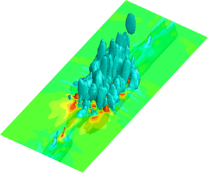
The development of incipient turbulent spots is demonstrated further in figure 9, where the three-dimensional structure of Spot II is depicted by iso-surfaces of the x-component velocity fluctuation at 10 % (shown in coral) and −5 % (cyan) of the freestream velocity. Figures 9(a), 9(b) and 9(c) correspond to the spot structure at x = 350, 380 and 400 mm, respectively. They demonstrate that the incipient turbulent spot was composed of a number of low-speed pillars that were anchored at the wall, which stretched out to the edge of the boundary layer. A high-speed region of the turbulent spot was also visible near the wall in between the low-speed pillars. These pillars represent the low-speed regions that were pumped up within each hairpin-like structures of the incipient turbulent spot. The structural development of an incipient turbulent spot shown in figure 9 reveals that the number of hairpin-like structures increased in both the streamwise and spanwise directions during the development. Low-speed pillars of incipient turbulent spots seem to be amalgamated at x = 400 mm (see figure 9c), which suggested that hairpin-like structures merged together during the spot development. The early development of turbulent spots that is shown in figure 9 is similar to that of Wu et al. (Reference Wu, Moin, Wallace, Skarda, Lozano-Durán and Hickey2017) in their DNS simulation of the turbulent boundary layer during transition.

Figure 9. Three-dimensional structure of Spot II depicted by iso-surfaces of ensemble-averaged x-component velocity fluctuations at 10 % (coral) and −5 % (cyan) of the freestream velocity, where colour contour slices at y = 1 mm are superimposed: (a) x = 350 mm; (b) x = 380 mm; (c) x = 400 mm.
Figures 10(a), 10(b) and 10(c) present the streamwise velocity fluctuations in the near-wall region (y = 0.5 mm) at x = 350, 380 and 400 mm, respectively, showing the downstream development of incipient turbulent spots. They show that Spot I decayed downstream, and its initial disturbance nearly disappeared by x = 400 mm. Meanwhile, Spot II developed downstream by generating a large number of high-frequency spikes. These spikes were positively skewed, which suggested that they were associated with a downwash of higher momentum fluid towards the wall. A similar development of Spot III is shown in figures 10(a), 10(b) and 10(c), although the development of this turbulent spot seemed to be slower than that of Spot II. The main difference between Spot II and Spot III was in the number of initial disturbances above the critical intensity. While Spot II had five velocity pulses in the initial disturbance, Spot III only had two. It seems, therefore, the speed of development of incipient turbulent spots depends on the number of velocity pulses or the duration of the initial disturbance.

Figure 10. Streamwise velocity signals (a single realisation) in the boundary layer at y = 0.5 mm, showing the downstream development of Spot I, II and III: (a) x = 350 mm, (b) x = 380 mm, (c) x = 400 mm.
The downstream change in the turbulence energy distribution within incipient turbulent spots can be studied by wavelet spectra using Matlab. Here, we used generalised Morse wavelets defined by  ${\varPsi _{P,\gamma }}(\omega ) = U(\omega ){a_{P,\gamma \textrm{\; }}}{\omega ^{{P^2/ \gamma}}}{\textrm{e}^{ - {\omega ^\gamma }}}$ in the frequency domain $\omega $, where $U(\omega )$ is the unit step function and ${a_{P,\gamma }}$ is a normalising constant (Lilly & Olhede Reference Lilly and Olhede2012). The symmetry parameter and the time-bandwidth product were set to γ = 3 and P 2 = 60, respectively. Figures 11(a), 11(b) and 11(c) show the wavelet spectra of the streamwise velocity signals in figures 10(a), 10(b) and 10(c), respectively. Figure 11(a) shows that the turbulence energy of Spot II and Spot III at x = 350 mm was contained between f = 0.5 and 2 kHz. With a downstream development of incipient turbulent spots, the wavelet spectrum spread to cover a wider frequency range up to f = 3 kHz. At x = 400 mm, much of the turbulence energy within Spot II and Spot III can be found between f = 1 and 3 kHz, see figure 11(c), as a result of high-frequency spikes being generated within incipient turbulent spots (see figure 10c). Figure 11 clearly shows that the turbulence energy in Spot I had nearly disappeared by x = 400 mm.

Figure 11. Wavelet spectra of streamwise velocity signals (a single realisation) in the boundary layer at y = 0.5 mm, showing the downstream development of Spot I, II and III: (a) x = 350 mm, (b) x = 380 mm, (c) x = 400 mm.
Figures 12(a), 12 (b) and 12(c) are similar to figures 10(a), 10(b) and 10(c), which show the streamwise velocity fluctuations at x = 350, 380 and 400 mm, respectively, near the edge of the boundary layer at y = 1.5 mm. Again, an increase in the number of high-frequency spikes was evident for Spot II and Spot III, while the initial disturbance was almost gone by x = 400 mm for Spot I. In contrast to figure 10, the high-frequency spikes at y = 1.5 mm were negatively skewed, which suggested that they were associated with an upwash of lower momentum fluid from the near-wall region. The downstream development of this low momentum region is clearly seen in figure 6. A strong shear layer between the low-speed region and the high-speed region produces high frequency velocity spikes (Wygnanski et al. Reference Wygnanski, Sokolov and Friedman1976) as we observe in figures 10 and 12. Figures 10 and 12 also show that velocity pulses within the structure started to shape into an envelope of turbulent spots at around x = 400 mm. This could be a result of a beating effect of high-frequency velocity pulses generated within the developing spot structure, which is similar to the generation process of very large-scale motions (VLSMs) from the hairpin packets in a turbulent boundary layer (Sharma & McKeon Reference Sharma and McKeon2013).

Figure 12. Streamwise velocity signals (a single realisation) in the boundary layer at y = 1.5 mm, showing the downstream development of Spot I, II and III: (a) x = 350 mm, (b) x = 380 mm, (c) x = 400 mm.
The wavelet spectra of streamwise velocity signals at y = 1.5 mm are shown in figures 13(a), 13(b) and 13(c) at x = 350, 380 and 400 mm, respectively. The turbulence energy of Spot I was reduced downstream very quickly as shown in figures 13(a), 13(b) and 13(c). However, the turbulence energy of Spot II and Spot III near the edge of boundary layer, which was initially concentrated between f = 1 kHz and 3 kHz owing to high-frequency spikes as shown in figure 12(a), shifted towards lower frequency downstream between f = 0.5 and 2.5 kHz at x = 380 mm and then to between f = 0.5 and 2 kHz at x = 400 mm. This shift of turbulence energy coincided with the formation of a turbulent spot envelope, as observed in figures 12(b) and 12(c). Indeed, we observed a low frequency peak (175 Hz) in the wavelet spectrum of Spot III at x = 400 mm in figure 13(c), which corresponded to the duration (6 ms) of the turbulent spot envelope being formed as shown in figure 12(c). A similar downshift in energy peak frequency was observed by Casper et al. (Reference Casper, Beresh, Henfling and Spillers2014a), who used the wavelet transform of wall-pressure traces to identify the location of turbulent spots on a 7° hypersonic cone.

Figure 13. Wavelet spectra of streamwise velocity signals (a single realisation) in the boundary layer at y = 1.5 mm, showing the downstream development of Spot I, II and III: (a) x = 350 mm, (b) x = 380 mm, (c) x = 400 mm.
Integral boundary-layer parameters, which include the displacement thickness δ*, the momentum thickness θ and the shape factor H, at x = 350, 380 and 400 mm are given in figures 14(a), 14(b) and 14(c), respectively. We observe that δ* and θ increased and the shape factor H = δ*/θ reduced as expected with the development of the boundary layer downstream. We can also observe that the integral parameters δ* and θ increased within incipient turbulent spots at each downstream location. Here, the relative increase in the momentum thickness within incipient turbulent spots was greater than that of the displacement thickness, therefore the shape factor H = δ*/θ was reduced. For example, the shape factor in Spot II was reduced to H = 1.9, 1.6 and 1.4 at x = 350, 380 and 400 mm, respectively, as shown in figures 14(a), 14(b) and 14(c). Therefore, the boundary layer flow within Spot II was already fully developed turbulence at x = 400 mm as the shaper factor reached to H = 1.4. The shape factor of the boundary layer outside incipient turbulent spots was reduced from H = 2.5 at x = 350 mm to H = 2.15 at x = 400 mm. This suggested that the ‘non-turbulence’ region of the boundary layer was already affected by the development of incipient turbulent spots even when the intermittency factor was only 22 % at x = 400 mm. It is interesting to observe that the shape factor of the boundary layer at this streamwise location was reduced from H = 2.15 to H = 1.4 very quickly when the front (downstream end) of the turbulent spot approached. However, the process of getting back to the ‘laminar’ region from the ‘turbulent’ region at the back (upstream end) of the turbulent spot, which is called the ‘calmed region’ by Schubauer & Klebanoff (Reference Schubauer and Klebanoff1956), was much slower. This arose from the elongated high-speed region affecting the ‘laminar’ region.

Figure 14. Integral boundary-layer parameters: (a) x = 350 mm; (b) x = 380 mm; (c) x = 400 mm.
Ensemble-averaged velocity profiles of the boundary layer between t = 113 and 130 ms are given in figure 15, which show the temporal structure of Spot II at x = 400 mm. Here, the boundary layer profiles are shown from left to right with an interval of 1 ms. This indicates that the boundary layer starts to develop a strong inflexional profile at t = 115 ms only a few milliseconds after the spot front had passed. Then, a velocity retardation region develops, moving towards the boundary-layer edge for the next 3 ms (t = 116–118 ms). This is followed by a flow acceleration near the wall. These temporal changes in the boundary-layer profile within Spot II can be further examined by the velocity fluctuations recorded between 110 and 130 ms at y = 0.2, 0.5, 1.0, 1.5, 2.0 and 2.6 mm, as shown on the right-hand side of the figure. Here, the velocity fluctuations were mostly negative away from the wall (y > 1.5 mm) and positive close to the wall (y < 0.5 mm), which suggested that a strong shear layer was created at around y = 1 mm by the inflexional velocity profile. This seems to be the location where the turbulence energy was produced in the boundary layer to maintain turbulent spots. This behaviour of turbulence energy generation in turbulent spots is very similar to the burst events in the turbulent boundary layer, where the ejection event (−u and +v velocity fluctuations) is followed by the sweep event (+u and -v velocity fluctuations), see figure 9 of Blackwelder & Kaplan (Reference Blackwelder and Kaplan1976).

Figure 15. Ensemble-averaged velocity profiles of the boundary layer at x = 400 mm. Solid lines are perturbed velocity profiles in Spot II between 110 and 130 ms at an interval of 1 ms, while dotted lines indicate the ‘laminar’ velocity profile outside incipient turbulent spots (t = 105 ms). The velocity fluctuations in Spot II between 110 and 130 ms are shown on the right at y = 0.2, 0.5, 1.0, 1.5, 2.0 and 2.6 mm (from bottom to top).
4. Conclusions
An experimental investigation was carried out in an extremely low-turbulence wind tunnel to study the early development of artificially initiated turbulent spots in a laminar boundary layer over a flat plate. A good data reproducibility allowed us to observe fine structural details that have not been seen before. Only portions of the velocity disturbances that are greater than a threshold value of approximately 10 % of the freestream velocity were able to develop downstream while the others decayed. This agrees with the finding of previous studies (Elder Reference Elder1960; Wygnanski et al. Reference Wygnanski, Sokolov and Friedman1976), which indicated that only disturbance above a ‘critical intensity’ will breakdown to turbulence to form turbulent spots. However, the threshold value in our study is much lower than that of the critical intensity obtained before.
Initial velocity disturbances, whose frequencies were outside the neutral stability curve of the boundary layer, quickly developed into hairpin-like structures that multiplied downstream, which increased the width, length and height of the incipient turbulent spots. Eventually, they developed into fully developed turbulent spots very similar to those studied by Zilberman et al. (Reference Zilberman, Wygnanski and Kaplan1977). As they develop downstream, there is a build-up of the low-speed region in the outer region of the boundary layer, accompanied by an elongation of the high-speed region near the wall. A strong shear layer is therefore created between the low-speed and the high-speed regions of developing turbulent spots, where high-frequency velocity spikes are generated. This seems to be the location where the turbulence energy is produced to maintain the turbulent spots. The behaviour of turbulence energy generation within a turbulent spot is very similar to the burst events in the turbulent boundary layer, where ejection events are followed by sweep events (Blackwelder & Kaplan Reference Blackwelder and Kaplan1976).
Iso-surfaces of the x-component of the velocity fluctuations show that developing turbulent spots consist of a number of low-speed pillars that are anchored at the wall, which stretch out to the edge of the boundary layer. The high-speed region of the turbulent spot is also visible near the wall in between the low-speed pillars. These pillars represent the low-speed regions that are pumped up within each hairpin vortex of the incipient turbulent spot. The sequence of structural changes demonstrates that the number of hairpin-like structures is increasing in both the streamwise and spanwise directions during the development to turbulent spots. The low-speed pillars of incipient turbulent spots seem to be amalgamated downstream, which suggests that hairpin-like structures merge together during the spot development. The early development of turbulent spots is similar to that of Wu et al. (Reference Wu, Moin, Wallace, Skarda, Lozano-Durán and Hickey2017) in their DNS simulation of the turbulent boundary layer during transition.
Hairpin-like structures were created by strong disturbances from an orifice in the form of pulsed jets (Sau & Mahesh Reference Sau and Mahesh2008, Reference Sau and Mahesh2010), not as a consequence of a secondary instability of the laminar boundary layer as observed by Borodulin et al. (Reference Borodulin, Gaponenko, Kachanov, Meyer, Rist, Lian and Lee2002). Once generated, however, these artificially initiated structures behaved very similarly to those resulting from the secondary flow instability, developing to turbulent spots by generating a large number of high-frequency spikes within. It has been shown that the turbulent spot inception mechanism during the bypass transition also involves packets of hairpin-like structures (Wu et al. Reference Wu, Moin, Wallace, Skarda, Lozano-Durán and Hickey2017). These results suggest that the hairpin-like structures are essential elements in the boundary layer transition.
The downstream change in the turbulence energy distribution within incipient turbulent spots was studied using wavelet spectra. With a development of turbulent spots downstream, the spectrum in the near-wall region spreads to cover higher frequency components, which reflects the generation of high-frequency spikes. These spikes are positively skewed, which suggests that they are associated with a downwash of higher momentum fluid towards the wall. In the outer region of the boundary layer, however, the spectrum shifts from higher frequency towards lower frequency downstream as a result of envelope formation of the incipient turbulent spots.
The shape factor of the boundary layer within developing turbulent spots reduces from the ‘laminar’ value (H = 2.15) to the ‘turbulent’ value (H = 1.4) very quickly when the spot front (downstream end) approaches. However, the process of getting back to the ‘laminar’ value from the ‘turbulent’ value at the back of the turbulent spots (upstream end), which is called the ‘calmed region’ by Schubauer & Klebanoff (Reference Schubauer and Klebanoff1956), is much slower. This arises from the elongation of the high-speed region near a wall during the downstream development of turbulent spots.
Acknowledgements
We acknowledge the helpful and constructive suggestions provided by anonymous referees.
Funding
This work was supported by EPSRC grant EP/M028690/1.
Declaration of interests
The authors report no conflict of interest.


 Open access