
The French mathematician Bertillon (Reference Bertillon1874) reasoned that the number of dizygotic (DZ) pairs would equal twice the number of twin pairs of unlike sexes. The remaining twin pairs in a sample would presumably be monozygotic (MZ). Weinberg (Reference Weinberg1902) restated this idea and the calculation has come to be known as Weinberg's differential rule (WDR). The basis of WDR is that DZ twin pairs should be equally likely to be of the same or the opposite sex. The small excess of males at birth (about 106:100) is not usually thought to affect the validity of the theory (Bulmer, Reference Bulmer1970). Departure of the sex ratio from 100 in either direction reduces the expected proportion of pairs of opposite sex, and thus the estimated number of DZ twin pairs of the same sex, in turn leading to an overestimation of the number of MZ twin pairs (Allen, Reference Allen, Gedda, Parisi and Nance1981; Boklage, Reference Boklage1985; Bulmer, Reference Bulmer1970; Little & Thompson, Reference Little, Thompson, MacGillivray, Campbell and Thompson1988).
Methods
Estimation of MZ and DZ Twinning Rates
The estimation is usually based on WDR, assuming that the probabilities of a male birth and female birth are equal and that the sexes within a twin set are independent. Although the probability of a male birth is greater than .5, the reliability of the WDR's assumptions has never been conclusively verified or rejected (Fellman & Eriksson, Reference Fellman and Eriksson2006). According to WDR, the total number of DZ twin maternities is twice the number of twin maternities with opposite-sex (OS) twin sets. The number of MZ twin sets is the difference between the number of same-sex (SS) and OS twin sets.
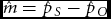
Let the total number of maternities be n, the number of SS twin sets be nS, and the number of OS twin sets be nO. One can assume that the distribution of nS, nO, and n − ns − no has a trinomial distribution. Let the probability for an OS twin maternity be pO, for an SS twin maternity pS and, consequently, the probability for other maternities 1 − pS − pO. Applying WDR, the MZ rate is m = pS − pO and the DZ rate is d = 2pO. According to the maximum likelihood theory, the estimators of transformed parameters are the corresponding transformations of the estimators of the initial parameters. Assuming that WDR holds, we can estimate pO and pS and use the formulae  $\hat m = \hat p_S - \hat p_O$ and $\hat d = 2\hat p_O$. This method does not solve if the proposed estimators $\hat m$ and $\hat d$ are unbiased estimators of the MZ and DZ rates, respectively. The unbiasedness depends on the reliability of Weinberg's assumptions. The likelihood function is
 \begin{equation}
L(p_S ,p_O ) = \left( {1 - p_S - p_O } \right)^{n - n_S - n_O } p_S^{n_S } p_O^{n_O } .\end{equation}
\begin{equation}
L(p_S ,p_O ) = \left( {1 - p_S - p_O } \right)^{n - n_S - n_O } p_S^{n_S } p_O^{n_O } .\end{equation}
The log-likelihood function is
 \begin{eqnarray*}
l(p_S ,p_O ) &=& (n - n_S - n_O )\ln (1 - p_S - p_O ) + n_S \ln (p_S )\nonumber\\
&& +\, n_O \ln (p_O ).
\end{eqnarray*}
\begin{eqnarray*}
l(p_S ,p_O ) &=& (n - n_S - n_O )\ln (1 - p_S - p_O ) + n_S \ln (p_S )\nonumber\\
&& +\, n_O \ln (p_O ).
\end{eqnarray*}After differentiation, we obtain
 \begin{eqnarray}
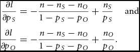
\frac{{\partial l}}{{\partial p_S }} &=& - \frac{{n - n_S - n_O }}{{1 - p_S - p_O }} + \frac{{n_S }}{{p_S }}\,\quad {\rm and}\nonumber\\
\frac{{\partial l}}{{\partial p_O }} &=& - \frac{{n - n_S - n_O }}{{1 - p_S - p_O }} + \frac{{n_O }}{{p_O }}.\end{eqnarray}
\begin{eqnarray}
\frac{{\partial l}}{{\partial p_S }} &=& - \frac{{n - n_S - n_O }}{{1 - p_S - p_O }} + \frac{{n_S }}{{p_S }}\,\quad {\rm and}\nonumber\\
\frac{{\partial l}}{{\partial p_O }} &=& - \frac{{n - n_S - n_O }}{{1 - p_S - p_O }} + \frac{{n_O }}{{p_O }}.\end{eqnarray}
The maximum of l(pS, pO) yields the estimators  $\hat p_S = \frac{{n_S }}{n}$ and $\hat p_O = \frac{{n_O }}{n}$, being unbiased, efficient, and asymptotically normal. To obtain the covariance matrix, we differentiate the formulae in (2) once more and obtain
 \begin{eqnarray*}
\frac{{\partial ^2 l}}{{\partial p_S^2 }} &=& - \frac{{n - n_S - n_O }}{{\left( {1 - p_S - p_O } \right)^2 }} - \frac{{n_S }}{{p_S^2 }},\quad\nonumber\\
\frac{{\partial ^2 l}}{{\partial p_O^2 }} &=& - \frac{{n - n_S - n_O }}{{\left( {1 - p_S - p_O } \right)^2 }} - \frac{{n_O }}{{p_O^2 }}\,,\quad {\rm and}\quad \,\nonumber\\
\frac{{\partial ^2 l}}{{\partial p_O \partial p_S }} &=& - \frac{{n - n_S - n_O }}{{\left( {1 - p_S - p_O } \right)^2 }}.
\end{eqnarray*}
\begin{eqnarray*}
\frac{{\partial ^2 l}}{{\partial p_S^2 }} &=& - \frac{{n - n_S - n_O }}{{\left( {1 - p_S - p_O } \right)^2 }} - \frac{{n_S }}{{p_S^2 }},\quad\nonumber\\
\frac{{\partial ^2 l}}{{\partial p_O^2 }} &=& - \frac{{n - n_S - n_O }}{{\left( {1 - p_S - p_O } \right)^2 }} - \frac{{n_O }}{{p_O^2 }}\,,\quad {\rm and}\quad \,\nonumber\\
\frac{{\partial ^2 l}}{{\partial p_O \partial p_S }} &=& - \frac{{n - n_S - n_O }}{{\left( {1 - p_S - p_O } \right)^2 }}.
\end{eqnarray*}Now, E(nS) = npS and E(nO) = npO and, consequently,
 \begin{equation*}
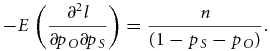
- E\left( {\frac{{\partial ^2 l}}{{\partial p_S^2 }}} \right) = \frac{{n\left( {1 - p_O } \right)}}{{p_S \left( {1 - p_S - p_O } \right)}},
\end{equation*}
\begin{equation*}
- E\left( {\frac{{\partial ^2 l}}{{\partial p_S^2 }}} \right) = \frac{{n\left( {1 - p_O } \right)}}{{p_S \left( {1 - p_S - p_O } \right)}},
\end{equation*} \begin{equation*}
- E\left( {\frac{{\partial ^2 l}}{{\partial p_O^2 }}} \right) = \frac{{n\left( {1 - p_S } \right)}}{{p_O \left( {1 - p_S - p_O } \right)}}\,,
\end{equation*}
\begin{equation*}
- E\left( {\frac{{\partial ^2 l}}{{\partial p_O^2 }}} \right) = \frac{{n\left( {1 - p_S } \right)}}{{p_O \left( {1 - p_S - p_O } \right)}}\,,
\end{equation*}and
 \begin{equation*}
- E\left( {\frac{{\partial ^2 l}}{{\partial p_O \partial p_S }}} \right) = \frac{n}{{\left( {1 - p_S - p_O } \right)}}.
\end{equation*}
\begin{equation*}
- E\left( {\frac{{\partial ^2 l}}{{\partial p_O \partial p_S }}} \right) = \frac{n}{{\left( {1 - p_S - p_O } \right)}}.
\end{equation*} The information matrix for the estimators  $\hat p_S$ and $\hat p_O$ is
 \begin{eqnarray}
\bm{\rm I}\left( {\hat{p}_{S},\hat{p}_{O} } \right) = \left[{\begin{array}{cc}
{\displaystyle\frac{{n\left( {1 - p_{O} } \right)}}{{p_{S} \left( {1 - p_{S} - p_{O} } \right)}}} & {\displaystyle\frac{n}{{\left( {1 - p_{S} - p_{O} } \right)}}} \\[11pt]
{\displaystyle\frac{n}{{\left( {1 - p_{S} - p_{O} } \right)}}} & {\displaystyle\frac{{n\left( {1 - p_{S} } \right)}}{{p_{O} \left( {1 - p_{S} - p_{O} } \right)}}} \\
\end{array}} \right]\nonumber\\
\end{eqnarray}
\begin{eqnarray}
\bm{\rm I}\left( {\hat{p}_{S},\hat{p}_{O} } \right) = \left[{\begin{array}{cc}
{\displaystyle\frac{{n\left( {1 - p_{O} } \right)}}{{p_{S} \left( {1 - p_{S} - p_{O} } \right)}}} & {\displaystyle\frac{n}{{\left( {1 - p_{S} - p_{O} } \right)}}} \\[11pt]
{\displaystyle\frac{n}{{\left( {1 - p_{S} - p_{O} } \right)}}} & {\displaystyle\frac{{n\left( {1 - p_{S} } \right)}}{{p_{O} \left( {1 - p_{S} - p_{O} } \right)}}} \\
\end{array}} \right]\nonumber\\
\end{eqnarray}
and the covariance matrix is
 \begin{eqnarray}
&&\bm{\rm C}\left( {\hat{p}_S,\hat{p}_O } \right) = \bm{\rm I}^{ - 1} \left( {\hat{p}_S ,\hat{p}_O } \right)\nonumber\\
&&\quad = \frac{1}{n}\left[ {\begin{array}{cc}
{\displaystyle p_S \left( {1 - p_{S} } \right)} & { - p_{S} p_{O} } \\[4pt]
{\displaystyle - p_{S} p_{O} } & {p_{O} \left( {1 - p_{O} } \right)}
\end{array}}\right].\end{eqnarray}
\begin{eqnarray}
&&\bm{\rm C}\left( {\hat{p}_S,\hat{p}_O } \right) = \bm{\rm I}^{ - 1} \left( {\hat{p}_S ,\hat{p}_O } \right)\nonumber\\
&&\quad = \frac{1}{n}\left[ {\begin{array}{cc}
{\displaystyle p_S \left( {1 - p_{S} } \right)} & { - p_{S} p_{O} } \\[4pt]
{\displaystyle - p_{S} p_{O} } & {p_{O} \left( {1 - p_{O} } \right)}
\end{array}}\right].\end{eqnarray}
The estimators  $\hat p_S$ and $\hat p_O$ have the variances ${\rm Var}(\hat p_S ) = \frac{{p_S (1 - p_S )}}{n}$ and ${\rm Var}(\hat p_O ) = \frac{{p_O (1 - p_O )}}{n}$ and the correlation coefficient ${\rm Cor}\left( {\hat p_S ,\hat p_O } \right) = - \sqrt {\frac{{p_S p_O }}{{\left( {1 - p_S } \right)\left( {1 - p_O } \right)}}}$.
The linear transformations  $\hat m = \hat p_S - \hat p_O$ and $\hat d = 2\hat p_O$ are efficient and asymptotically normal and, if WDR holds, also unbiased. The estimators of these parameters are $\hat m = \hat p_S - \hat p_O = \frac{{n_S - n_O }}{n}$ and $\hat d = 2\hat p_O = \frac{{2n_O }}{n}$. The covariance matrix is
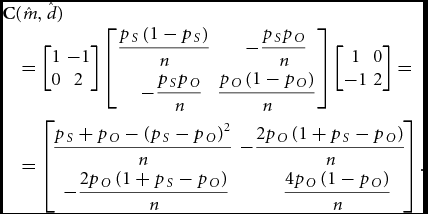 \begin{eqnarray}
\begin{array}{l}
\bm{\rm C}(\hat m,\hat d)\\
\quad = \left[\! {\begin{array}{*{20}c}
1 & { - 1} \\
0 & 2
\end{array}}\! \right]\left[\! {\begin{array}{*{20}c}
\hfill {\displaystyle\frac{{p_S \left( {1 - p_S } \right)}}{n}} & \hfill {\displaystyle - \frac{{p_S p_O }}{n}} \\[6pt]
\hfill {\displaystyle - \frac{{p_S p_O }}{n}} & \hfill {\displaystyle\frac{{p_O \left( {1 - p_O } \right)}}{n}}
\end{array}} \!\right]\left[\! {\begin{array}{*{20}c}
1 & 0 \\
{ - 1} & 2
\end{array}}\! \right] = \\[21pt]
\quad = \left[\!\! {\begin{array}{*{20}c}
\hfill {\displaystyle\frac{{p_S + p_O - \left( {p_S - p_O } \right)^2 }}{n}} & \hfill {\displaystyle - \frac{{2p_O \left( {1 + p_S - p_O } \right)}}{n}} \\[6pt]
\hfill {\displaystyle - \frac{{2p_O \left( {1 + p_S - p_O } \right)}}{n}} & \hfill {\displaystyle\frac{{4p_O \left( {1 - p_O } \right)}}{n}}
\end{array}}\!\! \right]. \\
\end{array}\nonumber\\[-8pt]
\end{eqnarray}
\begin{eqnarray}
\begin{array}{l}
\bm{\rm C}(\hat m,\hat d)\\
\quad = \left[\! {\begin{array}{*{20}c}
1 & { - 1} \\
0 & 2
\end{array}}\! \right]\left[\! {\begin{array}{*{20}c}
\hfill {\displaystyle\frac{{p_S \left( {1 - p_S } \right)}}{n}} & \hfill {\displaystyle - \frac{{p_S p_O }}{n}} \\[6pt]
\hfill {\displaystyle - \frac{{p_S p_O }}{n}} & \hfill {\displaystyle\frac{{p_O \left( {1 - p_O } \right)}}{n}}
\end{array}} \!\right]\left[\! {\begin{array}{*{20}c}
1 & 0 \\
{ - 1} & 2
\end{array}}\! \right] = \\[21pt]
\quad = \left[\!\! {\begin{array}{*{20}c}
\hfill {\displaystyle\frac{{p_S + p_O - \left( {p_S - p_O } \right)^2 }}{n}} & \hfill {\displaystyle - \frac{{2p_O \left( {1 + p_S - p_O } \right)}}{n}} \\[6pt]
\hfill {\displaystyle - \frac{{2p_O \left( {1 + p_S - p_O } \right)}}{n}} & \hfill {\displaystyle\frac{{4p_O \left( {1 - p_O } \right)}}{n}}
\end{array}}\!\! \right]. \\
\end{array}\nonumber\\[-8pt]
\end{eqnarray}
We rewrite (5) by using the parameters m and d and obtain
 \begin{eqnarray}
\bm{\rm C}(\hat{m},\hat{d}) = \frac{1}{n}\left[ {\begin{array}{cc}
\hfill {m(1 - m) + d} & \hfill { - d(1 + m)} \\
\hfill { - d(1 + m)} & \hfill {d(1 - d) + d}
\end{array}} \right].\end{eqnarray}
\begin{eqnarray}
\bm{\rm C}(\hat{m},\hat{d}) = \frac{1}{n}\left[ {\begin{array}{cc}
\hfill {m(1 - m) + d} & \hfill { - d(1 + m)} \\
\hfill { - d(1 + m)} & \hfill {d(1 - d) + d}
\end{array}} \right].\end{eqnarray}
We see that
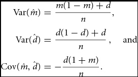 \begin{eqnarray}
{\rm Var}(\hat m) &=& \frac{{m(1 - m) + d}}{n},\quad\nonumber\\
{\rm Var}(\hat d) &=& \frac{{d(1 - d) + d}}{n}\,,\quad {\rm and}\quad\nonumber\\
{\rm Cov}(\hat m,\hat d) &=& - \frac{{d(1 + m)}}{n}.\end{eqnarray}
\begin{eqnarray}
{\rm Var}(\hat m) &=& \frac{{m(1 - m) + d}}{n},\quad\nonumber\\
{\rm Var}(\hat d) &=& \frac{{d(1 - d) + d}}{n}\,,\quad {\rm and}\quad\nonumber\\
{\rm Cov}(\hat m,\hat d) &=& - \frac{{d(1 + m)}}{n}.\end{eqnarray}
Bulmer (Reference Bulmer1970) presented slightly different approximate variance formulae. He assumed that the numbers of SS and OS twin sets are Poisson distributed but ignored that the numbers of OS and SS twin sets are correlated. His formulae are  ${\rm Var}(\hat m) = \frac{{m + d}}{n}$ and ${\rm Var}(\hat d) = \frac{{2d}}{n}$, yielding figures that, compared with ours, are slightly too large.
If  $\hat m$ and $\hat d$ are considered to be relative frequencies, one obtains the formulae ${\rm Var}(\hat m) = \frac{{m(1 - m)}}{n}$ and ${\rm Var}(\hat d) = \frac{{d(1 - d)}}{n}$, which are incorrect. The differences between the correct and incorrect formulae are positive and of the same order of magnitude (n − 1) as the correct ones and, consequently, the simple formulae should not be used, not even when the data sets are large. In addition, the erroneous variances are too small and may yield quite misleading test results and confidence intervals (CIs). For $\hat d$, the ratio between the correct variance estimate and the erroneous one is $\frac{{d(1 - d) + d}}{{d(1 - d)}} = \frac{{2 - d}}{{1 - d}} \approx 2$, and for $\hat m$ it is $\frac{{m(1 - m) + d}}{{m(1 - m)}} \approx \frac{{m + d}}{m}$. The latter ratio is approximately the ratio between the total and the MZ twinning rate and can be considerably larger than the ratio for $\hat d$.
Testing
According to (7), the estimators are negatively correlated and the correlation is usually rather strong. Therefore, the simultaneous testing of both MZ and DZ rates is to be preferred and a joint confidence region is better than two separate CIs. The information matrix is the inverse of the covariance matrix formula (6), which is
 \begin{eqnarray*}
&&\bm{\rm I}(\hat{m},\hat{d}) \nonumber\\
&&\quad = n\left[ {\begin{array}{cc}
\hfill {\frac{{d(1 - d) + d}}{{d\left( {2m - 3md - 2m^{2} + d - d^2 } \right)}}} & \hfill {\frac{{d(1 + m)}}{{d\left( {2m - 3md - 2m^{2} + d - d^{2} } \right)}}} \\[8pt]
\hfill {\frac{{d(1 + m)}}{{d\left( {2m - 3md - 2m^{2} + d - d^{2} } \right)}}} & \hfill {\frac{{m(1 - m) + d}}{{d\left( {2m - 3md - 2m^{2} + d - d^{2} } \right)}}}
\end{array}} \right]\nonumber\\
&&\quad = \left[ {\begin{array}{cc}
{I_{11} } & {I_{12} } \\
{I_{21} } & {I_{22} }
\end{array}} \right].
\end{eqnarray*}
\begin{eqnarray*}
&&\bm{\rm I}(\hat{m},\hat{d}) \nonumber\\
&&\quad = n\left[ {\begin{array}{cc}
\hfill {\frac{{d(1 - d) + d}}{{d\left( {2m - 3md - 2m^{2} + d - d^2 } \right)}}} & \hfill {\frac{{d(1 + m)}}{{d\left( {2m - 3md - 2m^{2} + d - d^{2} } \right)}}} \\[8pt]
\hfill {\frac{{d(1 + m)}}{{d\left( {2m - 3md - 2m^{2} + d - d^{2} } \right)}}} & \hfill {\frac{{m(1 - m) + d}}{{d\left( {2m - 3md - 2m^{2} + d - d^{2} } \right)}}}
\end{array}} \right]\nonumber\\
&&\quad = \left[ {\begin{array}{cc}
{I_{11} } & {I_{12} } \\
{I_{21} } & {I_{22} }
\end{array}} \right].
\end{eqnarray*}We construct the test statistic
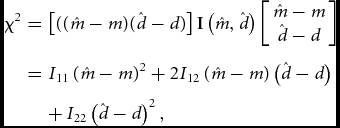 \begin{eqnarray}
{\rm \chi }^{2} &=& \left[ {((\hat{m} - m)(\hat{d} - d)} \right] \bm{\rm I}\left( {\hat{m},\hat{d}} \right)\left[ {\begin{array}{c}
{\hat{m} - m} \\
{\hat{d} - d}
\end{array}} \right]\nonumber\\ &=& I_{11} \left( {\hat{m} - m} \right)^2 + 2I_{12} \left( {\hat{m} - m} \right)\left( {\hat{d} - d} \right)\nonumber\\
&&+\, I_{22} \left( {\hat{d} - d} \right)^{2} ,\end{eqnarray}
\begin{eqnarray}
{\rm \chi }^{2} &=& \left[ {((\hat{m} - m)(\hat{d} - d)} \right] \bm{\rm I}\left( {\hat{m},\hat{d}} \right)\left[ {\begin{array}{c}
{\hat{m} - m} \\
{\hat{d} - d}
\end{array}} \right]\nonumber\\ &=& I_{11} \left( {\hat{m} - m} \right)^2 + 2I_{12} \left( {\hat{m} - m} \right)\left( {\hat{d} - d} \right)\nonumber\\
&&+\, I_{22} \left( {\hat{d} - d} \right)^{2} ,\end{eqnarray}
which is approximately χ2 distributed with 2 degrees of freedom. If we want to test the given hypothetical rates m and d, we observe  $\hat m$ and $\hat d$ and use the formula (8). It can also be used for the construction of a simultaneous confidence region for m and d. We observe that
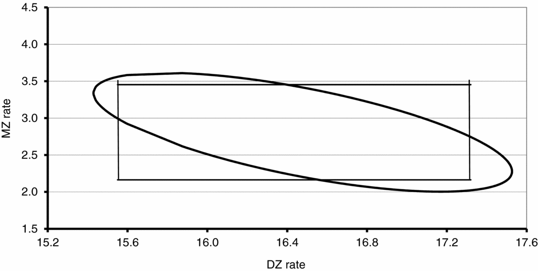
  $P( {I_{11} ( {\hat m - m} )^2 + 2I_{12} ( {\hat m - m} )( {\hat d - d} ) + I_{22} ( {\hat d - d} )^2 \!\! \le\! {\rm \chi }_\alpha ^2 } )\break \ge 1 - {\rm \alpha }$ is a confidence region for the parameters (m, d) with the confidence level 1 − α. The obtained region is an ellipse in the (m, d) plane (cf. Figure 1).

FIGURE 1 Confidence regions for MZ and DZ rates for Åland–Åboland, 1653–1949. Using  ${\rm SE}(\hat m)$ and ${\rm SE}(\hat d)$, we can construct the 95% CIs for the MZ rate and the DZ rate. For the Åland–Åboland data, we get the interval (2.16, 3.45) for m and (15.64, 17.32) for d, and the rectangle is constructed according to the individual CIs for m and d (Fellman & Eriksson, Reference Fellman and Eriksson2006).
For tests of a set of MZ and DZ rates, contingence tables cannot be used. An approximate test of a set of MZ or DZ rates can be performed in the following way. Consider MZ rates. Under the null hypothesis that the MZ rates are constant, being m for (t = 1, . . ., T),  ${\rm Var}(\hat m_t ) = \frac{{m(1 - m) + d}}{{n_t }}$, where nt is the sample size for t = 1, . . ., T. Define the weighted mean $\bar m = \sum_t {\frac{{n_t \hat m_t }}{{\sum {n_t } }}}$. Under the null hypothesis, $\bar m$ is the most efficient estimate of m. Consequently, ${\rm \chi }^2 = \frac{1}{c}\sum_{t = 1}^T {n_t \left( {m_t - \bar m} \right)^2 }$, where c = m(1 − m) + d, is asymptotically χ2 distributed with T − 1 degrees of freedom. An approximate χ2 test can be obtained if one uses $\hat c = \hat m(1 - \hat m) + \hat d$ as an estimate of c. For $\hat d$ one obtains a similar formula, but now c = d(1 − d) + d.
In numerical applications, the rates are usually given in per mille. This means that the theoretical variances should be scaled with a million and the estimators and standard errors with 1,000.
Results
Eriksson (Reference Eriksson1973, pp. 32 and 44) gave twinning data for the Åland Islands for 1653–1949 and for the neighboring archipelago of Åboland for 1655–1949.
Confidence Region
The total number of maternities is 178,055, the observed number of OS twin maternities is 1,467, and the observed number of SS twin maternities is 1,967. Using these data, we obtain (in per mille),  $\hat p_O = 8.24$, $\hat p_S = 11.05$, $\hat m = 2.81$, and $\hat d = 16.48$. We obtain
 \begin{eqnarray}
\bm{\rm C}\,(\hat m,\hat d) &=& \left[ {\begin{array}{*{20}c}
\hfill {0.1083} & \hfill { - 0.0928} \\
\hfill { - 0.0928} & \hfill {0.1836}
\end{array}} \right]\,\quad {\rm and}\quad\nonumber\\
\bm{\rm I}\left( {\hat m,\hat d} \right)& =& \left[ {\begin{array}{*{20}c}
\hfill {16.2993} & \hfill {8.2404} \\
\hfill {8.2404} & \hfill {9.6138}
\end{array}} \right].\end{eqnarray}
\begin{eqnarray}
\bm{\rm C}\,(\hat m,\hat d) &=& \left[ {\begin{array}{*{20}c}
\hfill {0.1083} & \hfill { - 0.0928} \\
\hfill { - 0.0928} & \hfill {0.1836}
\end{array}} \right]\,\quad {\rm and}\quad\nonumber\\
\bm{\rm I}\left( {\hat m,\hat d} \right)& =& \left[ {\begin{array}{*{20}c}
\hfill {16.2993} & \hfill {8.2404} \\
\hfill {8.2404} & \hfill {9.6138}
\end{array}} \right].\end{eqnarray}
Hence,  ${\rm Var}(\hat m) = 0.1083$ and ${\rm Var}(\hat d) = 0.1836$ and the standard errors are ${\rm SE}(\hat m) = 0.329$ and ${\rm SE}(\hat d) = 0.428$. The correlation between these estimators is −0.658. The 95% confidence region is $16.2993\left( {\hat m - m} \right)^2 + 16.4808\left( {\hat m - m} \right)\left( {\hat d - d} \right) + 9.6138\left( {\hat d - d} \right)^2 \le 5.99$. The confidence region is given in Figure 1.
Temporal Variations in the MZ and DZ Twinning Rates
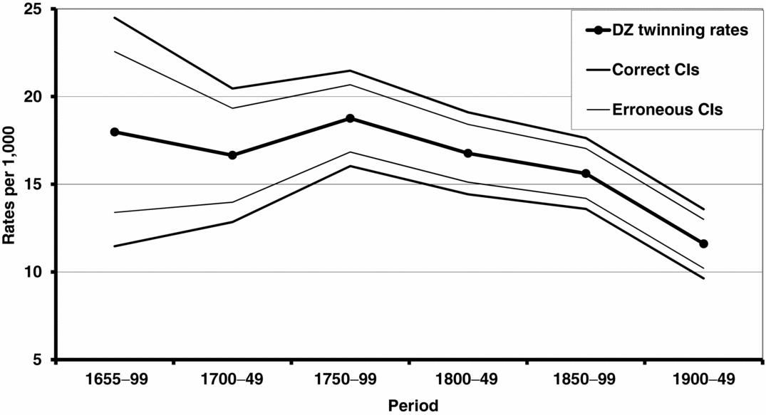
The MZ twinning rate estimated by WDR has increased in many western European countries simultaneously with a decline in DZ rates. It has been suggested that the increase in MZ twinning rates in developed countries could be due to the introduction of oral contraception in the 1960s. Fellman and Eriksson (Reference Fellman and Eriksson2006) noted that the increasing MZ rate observed in Åland–Åboland between 1653 and 1949 is statistically insignificant (χ2 = 5.92 with 5 degrees of freedom; p > .05) (see Figure 2). The temporal trend of the DZ twinning is given in Figure 3, and the temporal variation is statistically significant (χ2 = 26.14 with 5 degrees of freedom; p < .001), caused by a decreasing trend (Fellman & Eriksson, Reference Fellman and Eriksson2006).
FIGURE 2 Estimated MZ twinning rates, including the correct (95%) confidence band for Åland–Åboland, 1653–1949, according to the data in Eriksson (Reference Eriksson1973). To emphasize the use of the correct SE formulae, the erroneous confidence band is also included in the figure. The temporal variation is statistically insignificant (χ2 = 5.92 with 5 degrees of freedom; p > .05) (cf. Fellman & Eriksson, Reference Fellman and Eriksson2006).
FIGURE 3 Estimated DZ twinning rates, including the correct (95%) confidence band for Åland–Åboland, 1653–1949, according to the data in Eriksson (Reference Eriksson1973). To emphasize the use of the correct SE formulae, the erroneous confidence band is also included in the figure. The temporal variation is statistically significant (χ2 = 26.14 with 5 degrees of freedom; p < .001), caused by a decreasing trend (Fellman & Eriksson, Reference Fellman and Eriksson2006).
Discussion
One also has to consider the assumed independence between the sexes in a DZ twin pair. James (Reference James1971) observed an excess of DZ twin pairs of the same sex, primarily due to males, claiming that WDR underestimates the number of DZ twins. Fellman and Eriksson (Reference Fellman and Eriksson2006) have critically scrutinized WDR for the estimation of the MZ and DZ twinning rates. The basic assumptions for this rule are that the probability of a male birth is .5 and that the sexes within a DZ twin set are independent. These assumptions may be considered too simple, but their study indicates that WDR seems to be quite satisfactory, when large national birth register data are considered. Finally, the new standard errors for the estimated MZ and DZ rates should be used (cf. Figures 2 and 3). Especially, the standard errors for the MZ rate based on the correct formula are so large that variations other than random ones may be difficult to identify. If the WDR holds, the linearity indicates that the impact of external factors, such as maternal age and parity, seasonality, temporal effects, and ethnicity, has no disturbing effects on the analyses. Recently, Hardin et al. (Reference Hardin, Selvin, Carmichael and Shaw2008) analyzed twin registers from several countries and their analyses of WDR yielded satisfactory results.