


1. Introduction
Many flows of interest in the natural environment and engineering applications combine turbulent wakes and inertial particles. Turbulent wakes and inertial particles are of relevance where re-circulation, entrainment, energy deficits and pressure fluctuations affect the design and efficiency of wake-creating bodies such as wind turbines, aircraft, buildings and bridges (Cheynet et al. Reference Cheynet, Jakobsen, Snæbjörnsson, Angelou, Mikkelsen, Sjöholm and Svardal2017; Frej Vittale & Davenport Reference Frej Vittale and Davenport2017; Ali et al. Reference Ali, Hamilton, Cortina, Calaf and Cal2018; Hertwig et al. Reference Hertwig, Gough, Grimmond, Barlow, Kent, Lin, Robins and Hayden2019; de Jong Helvig et al. Reference de Jong Helvig, Vinnes, Segalini, Worth and Hearst2021; Smith et al. Reference Smith, Travis, Djeridi, Obligado and Cal2021). Cloud formation, industrial spray applications, combustion and air pollution are also of interest (Chandrakar et al. Reference Chandrakar, Cantrell, Ciochetto, Karki, Kinney and Shaw2017; Stodt, Kiefer & Fritsching Reference Stodt, Kiefer and Fritsching2019; Wei et al. Reference Wei, Zhang, Cai, Song, Bian, Xiao and Zhang2020; Gai et al. Reference Gai, Hadjadj, Kudriakov, Mimouni and Thomine2021). This study explores the effects of inertial particles in the wake behind a stationary porous disk in homogeneous isotropic turbulence (HIT).
For some time, the wakes behind porous disks have been studied as analogues to more complicated wakes such as parachutes and rotating wind turbines in single-phase flow applications. Roberts (Reference Roberts1980) studied drag coefficients of solid and porous disks with open area ratios of 2–33 per cent for parachute applications, and Aubrun et al. (Reference Aubrun, Loyer, Hancock and Hayden2013) compared wake properties of a porous disk with a rotating wind turbine model in wind tunnel experiments. Lignarolo et al. (Reference Lignarolo, Ragni, Ferreira and van Bussel2016) presented an experimental analysis comparing the near wakes of a wind turbine model and porous disk. Their results establish a good match between the turbine and the disk for velocity, pressure and enthalpy fields, but show differences in turbulence intensity and turbulent mixing. Aloui et al. (Reference Aloui, Kardous, Cheker and Ben Nasrallah2013) compared particle image velocimetry measurements of steady and unsteady wakes behind porous disks. Their proper orthogonal decomposition analysis showed that alternating vortices form in the unsteady wake.
In the case of wind energy, various porous disk designs have been studied in single-phase flows to approximate wind turbine wakes, as stationary disks are easier to simulate than rotating blades. (Martinez et al. Reference Martinez, Leonardi, Churchfield and Moriarty2012; Naderi & Torabi Reference Naderi and Torabi2017) A measurement campaign by Aubrun et al. (Reference Aubrun2019) compared uniform with non-uniform porous disks in nine different wind tunnels to investigate mean streamwise velocity and turbulence intensity profiles four diameters downstream of the disk. They found the results collapse reasonably well across facilities and that the non-uniform disk created a smaller velocity deficit and greater turbulence intensity in the centre of the wake. Camp & Cal (Reference Camp and Cal2016) developed a non-uniform porous disk, and compared the disk array with an array of rotating turbines and quantified the differences in the mean kinetic energy transport within the wakes. They ascertained the primary difference was in the spanwise mean velocity component in the near-wake region.
Others have studied various aspects of inertial particles in turbulent flows without wakes. Specifically, heavy particles at Stokes numbers of the order of unity, where a maximum coupling between particles and turbulence occurs, as described in Toschi & Bodenschatz (Reference Toschi and Bodenschatz2009). The mechanisms behind particle settling velocity modification in HIT are still being explored, and different studies have found both and increase and decrease in particle settling velocity, depending on various parameters and experimental and numerical conditions. For example, Aliseda et al. (Reference Aliseda, Cartellier, Hainaux and Lasheras2002) found the particle settling velocity to be larger than the quiescent fluid (an effect generally associated with the preferential sweeping mechanisms (Maxey Reference Maxey1987) and settling velocity enhancement increases with volume fraction, while Good et al. (Reference Good, Ireland, Bewley, Bodenschatz, Collins and Warhaft2014) found that nonlinear drag could induce settling hindering (associated with the loitering effect Nielsen Reference Nielsen1993) where regions of high velocity root-mean-square (r.m.s.) anisotropy generally coincide with regions of settling velocity reductions. Numerical simulations by Rosa et al. (Reference Rosa, Parishani, Ayala and Wang2016) found, however, that hindering by loitering rarely occurs unless particle horizontal motion is artificially blocked.
Settling velocity is also related to particle preferential concentration or clustering in turbulent flow structures. Sumbekova et al. (Reference Sumbekova, Aliseda, Cartellier and Bourgoin2016) and Obligado et al. (Reference Obligado, Cartellier, Aliseda, Calmant and de Palma2019) studied settling velocity and preferential concentration of inertial particles in HIT. Sumbekova et al. (Reference Sumbekova, Aliseda, Cartellier and Bourgoin2016) determined particles within clusters settle faster than particles in voids. This confirms observations by Aliseda et al. (Reference Aliseda, Cartellier, Hainaux and Lasheras2002). The same observation was also made by Huck et al. (Reference Huck, Bateson, Volk, Cartellier, Bourgoin and Aliseda2018), with a model to interpret the enhancement of settling as a collective ‘effective rheology’ effect. Obligado et al. (Reference Obligado, Cartellier, Aliseda, Calmant and de Palma2019) found cluster settling velocity has a strong dependence on the Taylor scale Reynolds number  $Re_{\lambda }$ or turbulence acceleration ratio, which is the ratio of the standard deviation of fluid acceleration fluctuations to gravity. Both Sumbekova et al. (Reference Sumbekova, Cartellier, Aliseda and Bourgoin2017) and Obligado et al. (Reference Obligado, Cartellier, Aliseda, Calmant and de Palma2019) show that clustering increases with volume fraction ( $\varPhi _{v}$) and $Re_\lambda$, and the mean size of clusters increases with $Re_\lambda$. However, Obligado et al. (Reference Obligado, Cartellier, Aliseda, Calmant and de Palma2019) (working at a fixed value of the free-stream velocity $U_\infty$) finds cluster size decreases with particle volume fraction $\varPhi _{v}$, while Sumbekova et al. (Reference Sumbekova, Cartellier, Aliseda and Bourgoin2017) found cluster size increases with $\varPhi _{v}$. Gustavsson, Vajedi & Mehlig (Reference Gustavsson, Vajedi and Mehlig2014) studied clustering of particles falling in turbulent flow and found the clustering is dependent on Stokes number and may be very anisotropic. Wang, Gu & Zheng (Reference Wang, Gu and Zheng2020) compared large and very large scale motions of single-phase flows with sand-laden flows with particles less than 10 $\mathrm {\mu }\mathrm {m}$ and particle volume fractions $<10^{-6}$. They found the streamwise turbulent kinetic energy is enhanced across all scales and that particles can affect turbulence at large scale structures.
Fewer studies have explored inertial particles in turbulent wakes. For instance, Fessler & Eaton (Reference Fessler and Eaton1999) found turbulence modification in a particle-laden flow over a backward facing step was a function of particle Stokes number and Reynolds number. More recently, Homann & Bec (Reference Homann and Bec2015) performed direct numerical simulation of inertial particles in the wake of a sphere and found particles form preferential concentrations in the wake. They found a region downstream of the sphere where particle concentration exceeds the inflow and suggest this is due to ejections of particles from detached and advected vortices.
This study aims to characterize the behaviour of inertial particles in the axisymmetric turbulent wake of a porous disk. This is a first step toward answering the question if and how stationery disks can be used as analogues to rotating turbines in the presence of inertial particles. As this is a first study on the subject, the focus is on the HIT incoming flow case. The persistence of the wake, how particles are entrained, particle discrimination by size, and particle settling velocity are studied. To the authors’ knowledge, this is the first experimental study on the coupling of inertial particles with a self-similar, large  $Re_\lambda$ flow behind a porous disk generator. The experimental set-up and data collection techniques are presented in § 2, and results are presented in § 3. The application of the analysis techniques and discussion follow in § 4, and concluding remarks on the implications are given in § 5.
2. Experimental set-up
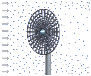
Experiments were conducted at the Université Grenoble Alpes at Laboratoire des Ecoulements Géophysiques et Industriels (LEGI) in the Lespinard Wind Tunnel. The closed-circuit wind tunnel test section is 4 m long with a cross-sectional area of  $0.75\,{\rm m} \times 0.75\,{\rm m}$ as shown in figure 3. Figure 1 shows the passive spray grid with 36 water misting nozzles (0.4 mm diameter) at the tunnel inlet that inject water droplets into the tunnel flow. A stationary open grid is located 15 cm upstream of the spray grid to override and mix the turbulence added by the injectors, and the combined grids produce turbulence intensity of the order of 2.4 %–3.0 %. A 150 bar pump supplied water to the spray grid, producing a uniform spray of poly-disperse water droplets with most probable diameters between 40–50 $\mathrm {\mu }$m. Water volumetric flow rate was controlled with a manual variable regulator and data were collected after the water flow rate, humidity and tunnel velocity reached steady state.

Figure 1. Disk model (a) and wind tunnel passive grid and spray grid (b).
A non-uniform porous disk attached to a 12.7 mm diameter aluminium tube was mounted in the wind tunnel and attached at the tunnel floor as shown in figures 3 and 1. The disk has a diameter of  $D=120$ mm, a thickness of 3.175 mm, a porosity of approximately 56 % and a tunnel blockage ratio of 1.57 % including the mounting tube. A small blockage ratio allows unimpeded expansion of the wakes within the tunnel. Holes in the disk range from 0.05–8.5 mm in size (refer to figure 2 for disk geometry). The disk was designed by Camp & Cal (Reference Camp and Cal2016) and the porosity varies radially to mimic the design of a wind turbine rotor.

Figure 2. Porous disk front and side views.

Figure 3. Schematic of wind tunnel experimental set-up, side view. (Schematic is not to scale.) Note that the measurement location is fixed at 3 m downstream of the grid and the disk model was moved for near- and far-wake measurements. Grey boxes represent PIV measurement regions and green points represent PDI and hot-wire measurement locations;  $D$ is the diameter of the disk. (Smith et al. Reference Smith, Travis, Djeridi, Obligado and Cal2021).
Hot-wire anemometry (HWA), phase Doppler interferometry (PDI) and particle image velocimetry (PIV) measurements were taken of the background flow (i.e. a passive grid flow with no wake) and compared with locations at one disk diameter ( $1D$) and 9.6 disk diameters ( $9.6D$) downstream of the disk to analyse characteristics of different flow regimes in the wake. The disk was positioned such that the measurement location was always 3 m downstream of the grid, thus assuring the same amount of background turbulence intensity. The disk was positioned in the centre of the tunnel cross-section for the HWA and PDI measurements, and 20 cm from the tunnel wall for the PIV measurements. The off-centre location of the disk for PIV measurements was due to hardware mounted to the top outer side of the tunnel preventing a central placement of the laser optic.
2.1. Characterization of the turbulence in the wake
The inflow conditions without inertial particles were characterized with HWA measurements using a Dantec Streamline constant temperature anemometer with a tungsten wire probe. The Pt-W 55P01 type probe had a sensing length of 1.25 mm and a wire diameter of 5  $\mathrm {\mu }$m. Data acquisition time was 300 s at either 20 kHz or 35 kHz at constant temperature and pressure, and velocities were calculated using King's law and Taylor's hypothesis. Adequate resolution was achieved to resolve the Kolmogorov length scale $\eta$, as $\kappa _{{max}}\eta \geq 1$, where $\kappa _{{max}}$ is the highest resolvable wavenumber $(\mathrm {rad}\,\mathrm {m}^{-1})$, estimated as $2 {\rm \pi}F_{s}/U_{\infty }$ with $F_{s}$ the sampling frequency (Hz) and $U_{\infty }$ the mean velocity $(\mathrm {m} \, \mathrm {s}^{-1})$ (assuming Taylor's hypothesis). To quantify turbulence in the absence of particles, the hot-wire was aligned vertically with the centre of the disk at 36.5 cm from the tunnel wall and floor. Measurements were taken in the tunnel at 3 m downstream of the grid with no wake (no disk model), and in the near and far wakes at $1D$ and $9.6D$, respectively, for tunnel speeds $U_{\infty }$ = 2.6, 4.9, 8.4, 10.6, 12.0 and 15.8 $\mathrm {m} \, \mathrm {s}^{-1}$.
Table 1 presents the following turbulence statistics calculated for the background flow (grid-generated turbulence but with no wake):
 \begin{gather} Re_{D} = U_{\infty} D/\nu, \end{gather}
 \begin{gather} Re_{\lambda} = \sigma_{u}\lambda / \nu, \end{gather}
 \begin{gather} L_{int} = \int_{0}^{r_0} \rho(r)\,\mathrm{d}r, \end{gather}
 \begin{gather} \lambda=\sqrt{(15\nu(\sigma_{u})^2)/\varepsilon}, \end{gather}
 \begin{gather} \eta=(\nu^3/\varepsilon)^{1/4}, \end{gather}
 \begin{gather} \varepsilon = \int_{0}^{\infty} 15 \nu k_{1}^{2} E_{11}\,{\rm d}k_{1}, \end{gather}
 \begin{gather} C_{\varepsilon}=\varepsilon L_{int} / \sigma_{u}^3, \end{gather}
where  $Re_{D}={\rm disk}$ diameter Reynolds number, $Re_{\lambda }=$ Taylor scale Reynolds number, $L_{int}=$ integral length scale, $\lambda =$ Taylor micro-scale, $\eta =$ Kolmogorov length scale, $\varepsilon =$ turbulent dissipation rate and $C_{\varepsilon }=$ dissipation constant. Other parameters include $\rho (r)=$ longitudinal auto-correlation function, $r_0$ corresponds to $\rho (r_0)=1/e$, $\sigma _{u}=$ r.m.s. of the streamwise velocity fluctuations, $E_{11}=$ streamwise power spectral density, $k_{1}=$ wavenumber of the fluctuating velocity signal, $U_{\infty }=$ free-stream velocity at $x=1$ m, $D=$ disk diameter and $\nu =$ kinematic viscosity of air.
Table 1. Calculated turbulence statistics for the background flow.

Figure 4 shows the normalized power spectral density (PSD) normalized with the velocity variance ( $\sigma _{u})^2$ as a function of wavenumber $\kappa$ for the measured instantaneous velocities for the background flow and disk wake locations at $1D$ and $9.6D$ downstream. The presence of the wake increases the dissipation wavenumber cutoff, with the largest cutoff in the near wake at $1D$. This indicates the wake is increasing energy dissipation and producing smaller eddies than the background flow. The inertial range is globally much clearer in the far wake at $9.6D$ where turbulence is enhanced. The low frequency peak at $1D$ is of the order of 2 cm, which is the size of the hub in the centre of the disk.

Figure 4. Normalized PSD as a function of wavenumber  $\kappa$ at different free-stream tunnel speeds from hot-wire measurements for (a) background flow, (b) $1D$ and (c) $9.6D$ wake locations. The $k^{-5/3}$ line represents the Kolmogorov spectrum.
HWA calculations are plotted for tunnel speeds  $U_{\infty } =$ 4.9, 8.3, 10.6, 12.0 and 15.8 $\mathrm {m} \, \mathrm {s}^{-1}$. Figure 5 shows turbulence intensity vs the local mean streamwise velocity $\bar {U}$ for the background flow and wake locations at $1D$ and $9.6D$ downstream of the disk. The local mean velocity $\bar {U}$ is reduced by approximately 54 %–66 % in the near wake at $1D$ and 7 %–19 % in the far wake at $9.6D$. Turbulence intensity remains fairly constant for the background flow and far wake, and varies with $\bar {U}$ in the near wake, indicating the near wake is a highly turbulent and non-homogeneous region. Figures 4(b) and 5 confirm that that near-wake flow is within the recirculation bubble and therefore cannot be characterized via HWA in figures 6–11, as measurements are contaminated by velocity components other than the streamwise one.

Figure 5. Turbulence intensity  $\sigma _{u} / \bar {U}$ vs mean velocity $\bar {U}$ for the background flow and disk wakes at $1D$ and $9.6D$ downstream.

Figure 6. Taylor scale Reynolds number  $Re_{\lambda }$ as a function of local mean velocity $\bar {U}$ for the background flow and wake at $9.6D$ at tunnel speeds $U_{\infty } =$ 1.3, 4.9, 8.3, 10.6, 12.0 and 15.8 $\mathrm {m} \, \mathrm {s}^{-1}$.

Figure 7. The turbulent dissipation rate  $\varepsilon$ vs the Taylor scale Reynolds number $Re_{\lambda }$ for the background flow and wake locations at $1D$ and $9.6D$ for tunnel speeds $U_{\infty } =$ 1.3, 4.9, 8.3, 10.6, 12.0 and 15.8 $\mathrm {m} \, \mathrm {s}^{-1}$.

Figure 8. Comparison of the turbulent dissipation rate  $\varepsilon$ vs the Taylor scale Reynolds number $Re_{\lambda }$ for the background flow and far wake at $9.6D$ at tunnel speeds $U_{\infty } =$ 1.3, 4.9, 8.3, 10.6, 12.0 and 15.8 $\mathrm {m} \, \mathrm {s}^{-1}$.

Figure 9. Transverse Taylor microscale  $\lambda$, as a function of the Taylor scale Reynolds number $Re_{\lambda }$ for the background flow and wake at $9.6D$ at tunnel speeds $U_{\infty } = 1.3$, 4.9, 8.3, 10.6, 12.0 and 15.8 $\mathrm {m} \, \mathrm {s}^{-1}$.

Figure 10. The Kolmogorov length scale  $\eta$ vs the Taylor scale Reynolds number $Re_{\lambda }$ for the background flow and the wake at $9.6D$ at tunnel speeds $U_{\infty } = 1.3$, 4.9, 8.3, 10.6, 12.0 and 15.8 $\mathrm {m} \, \mathrm {s}^{-1}$.

Figure 11. Values of  $C_{\varepsilon }$ and $L_{int}/\lambda$ are plotted vs the Taylor scale Reynolds number $Re_{\lambda }$ for the background flow and the wake at $9.6D$ at tunnel speeds $U_{\infty } = 1.3$, 4.9, 8.3, 10.6, 12.0 and 15.8 $\mathrm {m} \, \mathrm {s}^{-1}$.
Figures 6–11 compare turbulence statistics (see table 1) for the far wake at  $9.6D$ with the background flow conditions. Figure 6 shows the Taylor scale Reynolds number $Re_{\lambda }$ as a function of local mean velocity $\bar {U}$. For both cases $Re_{\lambda }$ increases with increasing $\bar {U}$.
Figure 7 shows  $\varepsilon$, where the dissipation rate at $1D$ is an order of magnitude greater than the background flow and the far wake. Figures 7 and 8 show $\varepsilon$ also increases with increasing $Re_{\lambda }$.
Figure 9 shows the transverse Taylor microscale  $\lambda$ as a function of $Re_{\lambda }$. $\lambda$ represents the intermediate length scale at which viscosity significantly affects turbulent eddies, and values of $\lambda$ are smaller in the wake indicating the wake is generating more turbulent dissipation. The value of $Re_{\lambda }$ is greater in the wake due to greater $\sigma _{u}$ of the turbulent signal. In both cases $\lambda$ decreases with increasing $Re_{\lambda }$ as higher velocities are also producing more turbulence.
The Kolmogorov length scale  $\eta$ is shown in figure 10 as a function of $Re_{\lambda }$. The value of $\eta$ decreases with increasing $Re_{\lambda }$ for both cases, as $\eta$ and $\lambda$ are linked by the exact relation: $\lambda /\eta = 15^{1/4}Re_{\lambda }^{1/2}$. For each $Re_{\lambda }$, $\eta$ is smaller in the wake as the disk injects energy to smaller scales where dissipation occurs.
Figure 11 compares the dissipation equation constant  $C_{\varepsilon }$ and $L_{int}/\lambda$ vs $Re_{\lambda }$. The value of $C_{\varepsilon }$ is larger for the background flow where it ranges from 0.83 to 1.4, these values are in agreement with values presented in Sreenivasan (Reference Sreenivasan1998) and Vassilicos (Reference Vassilicos2015). The value of $C_{\varepsilon }$ is reduced by approximately half in the wake where it ranges from 0.33–0.41. The value of $L_{int}/\lambda$ steeply increases with increasing $Re_{\lambda }$ for both cases, due to the decrease in $\lambda$ at higher $Re_{\lambda }$. The linear slopes of $L_{int}/\lambda$ agree with Kolmogorov's 1941 theory that $L_{int}/\lambda \sim C_{\varepsilon }Re_{\lambda }$, and that the background flow and far wake have HIT and the Taylor hypothesis holds.
HWA measurements presented in figures 6–11 show that in the absence of inertial particles, classical HIT scaling works reasonably well. The disk produces more turbulence, smaller eddies and greater dissipation of turbulent kinetic energy than the background flow.
2.2. Two-phase flow experiments – PDI methodology
Table 2 lists case parameters for the PDI measurements. Water was delivered to the spray grid at 1.7 and 2.0  $\mathrm {l} \, \mathrm {min}^{-1}$ and at three different free-stream tunnel velocities resulting in various global water volume fractions calculated as $\varPhi _{v}=Q_{L}/(Q_{L}+Q_{G})$, where $Q_{L}$ and $Q_{G}$ are the liquid and gas volumetric flow rates, respectively. The Stokes number based on the most probable particle diameter of 40.5 $\mathrm {\mu }{\rm m}$ (that remains approximately stable for all $U_\infty$ and $\varPhi _v$) was calculated for the background flow (no wake) as $St =\tau _{p}/\tau _{\eta } = (\rho _{p} d_{p}^2 \varepsilon ^{1/2})/(18 \rho _{f} \nu ^{3/2})$ and the minimum and maximum water volume fractions are listed for each tunnel velocity. This range of Stokes numbers ( $St \sim 1$) provides maximum coupling between turbulence and heavier inertial particles that can be centrifuged out of vortex cores and form clusters influenced by turbulent structures.
Table 2. PDI case parameters for figures 13 and 12.

The PDI measurement location is denoted with circles in figure 3 and was located 3 m downstream of the grid, 36.5 cm from the floor and receiver side of tunnel and 38.5 cm from the laser transmitter side. The PDI system remained stationary while the disk was positioned in the tunnel such that the PDI measurement location was centred behind the disk at  $1D$ and $9.6D$ downstream. PDI data were collected with an Artium Technologies PDI-200MD system, capable of detecting particle diameter ranges from 0.5–2000 $\mathrm {\mu }{\rm m}$ with a velocity range of $-100$ to $+300\,\mathrm {m}\,\mathrm {s}^{-1}$, with $\pm 0.2\,\mathrm {m}\,\mathrm {s}^{-1}$ accuracy. Two diode pumped solid state lasers with wavelengths of 532 and 473 nm were split into two beams of equal intensity with the 532 nm beam oriented to measure vertical velocity and particle diameter, and the 473 nm beam oriented to measure horizontal velocity. The transmitter and receiver were positioned on opposite sides of the tunnel and had focal lengths of 1000 and 500 mm respectively. The receiver aperture was 200 $\mathrm {\mu }{\rm m}$. Signals were analysed with the Artium advanced signal analyser with a maximum sampling frequency of 320 MHz and resolution of 0.01 % of sampling frequency; $500 \times 10^{3}$ signals were collected per case with the Automated Instrument Management System (AIMS) 5.2 software to assure good statistical convergence. Particle diameters and velocities were measured for water flow- rates of 1.7 and 2.0 $\mathrm {l} \, \mathrm {min}^{-1}$ at the free-stream tunnel speeds listed in table 2, leading to particle volume fraction varying in the range $\varPhi _{v}\in ([6-19] \times 10^{-6})$.
2.3. Two-phase flow experiments – PIV methodology
PIV measurements were taken with water flow rates of 1.2, 1.7 and 2.0  $\mathrm {l} \, \mathrm {min}^{-1}$ and non-inertial tracer particles ( $\varPhi _{v}=0$) at a constant tunnel fan speed as shown in table 3. Measurements were taken of the combined air–particle velocity by using the inertial particles as tracers in the two-phase flow cases. Tracer particles were used for the single-phase flow cases. Figures 14–20 compare tracer particle behaviour in the single-phase flow with the inertial particle behaviour in the two-phase flow. To prevent laser interference from water droplets adhering to the top inside tunnel window, a 12 mm angle was attached on the inside upper window upstream of the laser. The vertical laser sheet was aligned with the free stream and was centred with respect to the disk giving a velocity field in the $x$–
$x$– $y$ plane. Note that the wake is axisymmetric in the $x$–
$x$– $z$ plane, but not axisymmetric in the $x$–
$x$– $y$ plane due to the influence of the tube holding the disk. The model was painted black to prevent reflections, however, some reflections were still present resulting in a cropped region of interest for the near wake at $1D$. Regions of interest for the near and far wakes are shown as rectangles in figure 3. PIV data were collected with the use of a Litron LD30-527, double pulse, Nd:YLF laser with a frequency of 3.0 kHz, a wavelength of 527 nm and a $\Delta t$ of 295–310 $\mathrm {\mu }$s. For non-inertial tracer particles, the flow was seeded with two Antari alpha F-80Z smoke machines with Antari high density smoke Z-Fluid. For the inertial particle cases, the water droplets were used as seeding. A Phantom V2511 high speed camera with a 50 mm Nikon lens and resolution of $1280 \times 800$ pixels was set perpendicular to the laser sheet, and the camera captured images through an opening in the tunnel wall. The PIV grid size was $\Delta x/D = \Delta y/D = 21 \times 10^{-4}$ and 8000 pairs of images were analysed to generate converged turbulence statistics. It was found from approximately $10 \times 10^{3}$ snapshots that the number of images needed for convergence of mean velocity was below 2000. Non-inertial particle measurements were analysed with Dantec Dynamic Studio 9.7 PIV software, and inertial particle measurements were analysed with PIVLab, an open source software by Thielicke & Stamhuis (Reference Thielicke and Stamhuis2014).
Table 3. PIV Case Parameters for figures 14–20.

3. Results
3.1. Particle size and velocity distribution along the centreline of the wake
The following results were obtained using PDI within the wake of the disk and in the background flow. Figure 12 shows the probability density function (p.d.f.) of particle counts as a function of particle velocity for near and far wakes at a constant wind tunnel fan speed resulting in an average free-stream speed of 4.9  $\mathrm {m} \, \mathrm {s}^{-1}$. Symbols $\varPhi _{1.7}$ and $\varPhi _{2}$ represent water volume fractions of $10.1 \times 10^{-6}$ and $12.3 \times 10^{-6}$ respectively, where the subscripts refer to 1.7 and 2.0 $\mathrm {l} \, \mathrm {min}^{-1}$ water volumetric flow rates.

Figure 12. The p.d.f.s of particle counts as a function of streamwise particle velocity for one wind tunnel fan speed. Two volume fractions ( $\varPhi _{1.7}$ and $\varPhi _{2}$) and two wake locations ( $1D$ and $9.6D$) are compared with the background flow. Line colours represent different flow rates and wake locations, while line types indicate the wake vs background flow.
Particle velocities in figure 12 are reduced in the near wake by approximately 144 %–141 %, and are negative, indicating recirculation. This flow reversal confirms why the hot-wire measurements cannot accurately characterize the near wake at  $1D$. Particles in the far wake have a velocity reduction of 7.4 %–12.2 % confirming that the wake is still present at $9.6D$ downstream. Increasing the water volume fraction for each tunnel speed reduces the particle streamwise velocities as the bulk flow gains mass.
Figure 13 shows p.d.f.s of particle counts as a function of particle diameter for two different water flow rates (columns) and  $1D$ and $9.6D$ wake locations (rows) for three different wind tunnel speeds. Most probable particle diameters range from 13 $\mathrm {\mu }\mathrm {m}$ in the near wake to 41 $\mathrm {\mu }\mathrm {m}$ in the background flow. For all cases, diameters are 2–10 $\mathrm {\mu }{\rm m}$ larger for the higher flow rate, with smaller diameters at $1D$ (3–21 $\mathrm {\mu }{\rm m}$ difference). At $9.6D$ particle diameter distributions are similar between the wake and the background flow, with the most probable particle diameter between 30 and 41 $\mathrm {\mu }{\rm m}$. In contrast, the wake at $1D$ produces a much higher probability of particles around 17 $\mathrm {\mu }{\rm m}$, implying preferential trapping of smaller particles within the near-wake region. Local Stokes numbers in the near wake calculated with a particle diameter of 17 $\mathrm {\mu }{\rm m}$ range from 0.049 for $U_\infty \approx 3\, \mathrm {m}\,\mathrm {s}^{-1}$ to 0.17 for $U_\infty \approx 7.8\,\mathrm {m}\,\mathrm {s}^{-1}$, which are smaller than the Stokes numbers of the background flow. Particle trapping may be occurring in the wake at $1D$ as this was also seen at $1D$ in the wake of a model turbine by Smith et al. (Reference Smith, Travis, Djeridi, Obligado and Cal2021). Particle trapping could be confirmed in future experiments with particle tracking velocimetry. Figures 12 and 13 illustrate recirculation of small particles at $1D$, and that the wake still influences the particles at $9.6D$ downstream.

Figure 13. The p.d.f.s of particle counts as a function of particle diameter for wakes at  $1D$ and $9.6D$ (a,b and c,d), and water flow rates of 1.7 and 2.0 $\mathrm {l} \, \mathrm {min}^{-1}$ (a,c and b,d). Line colours represent three different wind tunnel speeds, and line types represent the wakes and background flows (no wake).
3.2. Velocity statistics of the global wake modulation through particle injection
Turbulence statistics calculated from PIV measurements are compared for inertial particles (water droplets) and sub-inertial particles (smoke) in near and far regions of the disk wake. Inertial particles were used as the seeding for PIV measurements to observe particle behaviour. Figures 14 and 15 show contour plots of various time-averaged normalized statistics at the same wind tunnel speed, which corresponds to  $Re_{\lambda }=88.7$ in the single-phase flow. Areas of interest span from $x/D = 0.75D$– $1.75D$ for the near wake, and $9.5D$– $11D$ for the far wake. Row $\varPhi _{0}$ shows contour plots of the single-phase flow wake; and rows $\varPhi _{1.2}$, $\varPhi _{1.7}$, and $\varPhi _{2}$ show contours of inertial particle behaviour in the wake with water flow rates of 1.2, 1.7, and 2 $\mathrm {l} \, \mathrm {min}^{-1}$ and corresponding particle volume fractions of $7.11 \times 10^{-6}, 10.1 \times 10^{-6}$ and $12.3 \times 10^{-6}$, respectively. The centre of the disk is at $y/D = 0$ and the flow is from the left. Each column in figure 14 represents the following normalized statistics: mean streamwise velocity $\bar {u}/U_{\infty }$, mean vertical velocity $\bar {v}/U_{\infty }$, and Reynolds stresses $\overline {u'u'}/U_{\infty }^2$, $\overline {u'v'}/U_{\infty }^2$ and $\overline {v'v'}/U_{\infty }^2$. Figure 15 shows the same quantities, but in the far wake.

Figure 14. Contour plots of the near wake at  $1D$. Normalized mean streamwise velocity $\bar {u}/U_{\infty }$, mean vertical velocity $\bar {v}/U_{\infty }$ and normalized mean Reynolds stresses $\overline {u'u'}/U_{\infty }^2$, $\overline {u'v'}/U_{\infty }^2$ and $\overline {v'v'}/U_{\infty }^2$ are shown in each column. Panels (a–e) $\varPhi _0$ represents single-phase flow with tracer particles and panels (f–j), (k–o) and (p–t) $\varPhi _{1.2}$, $\varPhi _{1.7}$ and $\varPhi _{2}$ represent two-phase particle velocity fields with increasing volume fractions with water flow rates of 1.2, 1.7 and 2 $\mathrm {l} \, \mathrm {min}^{-1}$ and volume fractions of $1.77 \times 10^{-6}, 10.3 \times 10^{-6}$ and $12.3 \times 10^{-6}$ respectively. Note that the colour scales vary so that spatial features can be identified and the flow is from the left.

Figure 15. Contour plots of the far wake at  $9.6D$. Normalized mean streamwise velocity $\bar {u}/U_{\infty }$, mean vertical velocity $\bar {v}/U_{\infty }$ and normalized mean Reynolds stresses $\overline {u'u'}/U_{\infty }^2$, $\overline {u'v'}/U_{\infty }^2$ and $\overline {v'v'}/U_{\infty }^2$ are shown in each column. Panels (a–e) $\varPhi _0$ represents single-phase flow with tracer particles and panels (f–j), (k–o) and (p–t) $\varPhi _{1.2}$, $\varPhi _{1.7}$ and $\varPhi _{2}$ represent two-phase particle velocity fields with increasing volume fractions with water flow rates of 1.2, 1.7 and 2 $\mathrm {l} \, \mathrm {min}^{-1}$ and volume fractions of $4.26 \times 10^{-6}, 6.03 \times 10^{-6}$ and $7.09 \times 10^{-6}$ respectively. Note that the colour scales vary so that spatial features can be identified and the flow is from the left.
In figure 14, the near wake  $\varPhi _{0}$ velocity remains positive at the core of the wake, with a distinct steep velocity gradient around $y/D\sim 0.5$, above which is the free stream where $\bar {u}/U_{\infty }$ is unity. The lower half of the wake does not have a distinct edge due to the influence of the tube that attaches the disk to the tunnel floor. In contrast to the single-phase flow, the inertial particles reverse direction where they are trapped and recirculated behind the disk. Inertial particles shift the top of the wake to $y/D > 0.7$. Particle $\bar {u}/U_{\infty }$ PIV measurements confirm particle recirculation in the near wake with regimes of negative $\bar {u}$, and reveal these regions grow in size with increasing volume fraction.
As shown in the second column of figure 14, the near-wake normalized mean vertical velocity  $\bar {v}/U_{\infty }$ remains negative (downward) for the $\varPhi _{0}$ case, with the maximum downward flow at $y/D \sim -0.5$. Inertial particles reveal recirculation with a band of negative $\bar {v}/U_{\infty }$ at the top of the wake at $y/D \sim 0.5$ and a band of positive $\bar {v}/U_{\infty }$ (upward) at the bottom of the wake at $y/D \sim -0.5$.
The third column of figure 14 displays the normal Reynolds stress  $\overline {u'u'}/U_{\infty }$, which represents the contributions of streamwise turbulence fluctuations to momentum within the single-phase flow wake. In the near wake, the single-phase flow normal stress is near zero at $y/D \sim 0.3$, and increases downward and upstream (left). The particle velocity fields show bands of normal stress at the top and bottom edges of the wake, at $y/D \sim \pm 0.5$. Interestingly, the middle volume fraction $\varPhi _{1.7}$ differs from the other particle cases, with greater stress in the lower band of the wake, and less stress in the upper band.
The fourth column of figure 14 shows shearing Reynolds stress  $\overline {u'v'}/U_{\infty }$, which represents vertical fluctuation influence on streamwise turbulent momentum for single-phase flows. In the near-wake single-phase flow, the shearing stress is negative at $y/D \sim 0.1$ and three bands of positive shear stress appear at $y/D \sim -0.2, -0.5$ and $-0.9$. The inertial particle velocity fields show pronounced bands of low and high $\overline {u'v'}/U_{\infty }$ with a negative band at $y/D \sim 0.5$ and a wider positive band at $y/D \sim -0.5$.
The column on the right in figure 14 shows  $\overline {v'v'}/U_{\infty }$, which is the vertical Reynolds normal stress and represents energy contributions within the single-phase flow wake from the vertical turbulent fluctuations. The single-phase flow $\overline {v'v'}/U_{\infty }$ in the near wake, is approximately zero above $y/D \sim 0.25$, and increases as you move downward and to the left. The near-wake particle velocity field $\overline {v'v'}/U_{\infty }$ forms bands at the top and bottom of the wake, but is less distinct than $\overline {u'v'}/U_{\infty }$, and increases with increasing volume fraction. In the near wake $\varPhi _{1.2}$ case, two distinct bands of higher $\overline {v'v'}/U_{\infty }$ are centred behind the disc at $y/D \sim 0.3$ and -0.3.
In figure 15, the far-wake single-phase flow ( $\varPhi _{0}$), the core tapers downward so that the centre of the wake core is around $y/D \sim -0.3$. The top edge of the wake is clearly defined and the bottom of the wake has moved lower than the region of interest, indicating the wake grows wider as it moves downstream. In the inertial particle cases, the far wake $\bar {u}/U_{\infty }$ is lower in magnitude and positive as particles move downstream. All three volume fractions have similar contours that show a reduction in $\bar {u}/U_{\infty }$ toward the bottom of the region of interest, suggesting the particle far wakes have shifted downward out of the region of interest. Figure 12 obtained with the PDI confirms that the wake is still present at $9.6D$, and the differences in particle velocity are small as one varies the volume fraction, which is in agreement with figure 14.
The far wake  $\bar {v}/U_{\infty }$ in figure 15, decreases with height for the $\varPhi _{0}$ case and a local minimum occurs below $y/D \sim -0.5$ and below $x/D \sim 10$. For the inertial particle cases, $\bar {v}/U_{\infty }$ is more negative at the top edge of the wake, and approaches but does not reach zero below $y/D \sim -0.5$.
In figure 15, the behaviour of  $\overline {u'u'}/U_{\infty }$ in the far wake single-phase flow is different than the near wake, where a band of higher $\overline {u'u'}/U_{\infty }$ is clearly visible at $y/D \sim 0.25$, and it increases as it moves downstream. Note that the vertical line of slightly higher values at $x/D \sim 10.2$ is due to a laser reflection. Generally, the far-wake inertial particle cases have lower magnitudes for the middle volume fraction $\varPhi _{1.7}$, and show larger bands of greater normal stress in the lower part of the region of interest below $y/D \sim -0.5$. All inertial particle cases have a thinner but distinct band of higher $\overline {u'u'}/U_{\infty }$ at $y/D \sim 0.5$. Inertial particle velocity fields have different structures than the single-phase flow, where particles tend to have greater $\overline {u'u'}/U_{\infty }$ at the top edge of the wake.
In the far wake in figure 15, the magnitude of the single-phase  $\overline {v'v'}/U_{\infty }$ is an order of magnitude lower than the near wake. In the single-phase flow, bands of positive and negative shear stress are wider with less defined edges as the wake expands downstream. The $\varPhi _{0}$ case has an upper band of negative shear stress centred at $y/D \sim 0.2$ and a lower band of positive shear stress centred at $y/D \sim -0.7$, with bands of zero shear stress at $y/D > 0.5$ and $\sim -0.25$. The far-wake particle velocity fields also have bands of negative shear stress at the top of the wake, and positive shear stress below, but these bands have moved away from the centre of the wake, with the upper band centred around $y/D \sim 0.53$ and less defined lower bands of positive shear stress starting below $y/D \sim -0.45$. Both the $\varPhi _{1.2}$ and $\varPhi _{1.7}$ cases have a band of zero shear stress at $y/D \sim 0$, but this band moves downward to $y/D \sim -0.3$ for the $\varPhi _{2}$ case.
In figure 15 far wake  $\varPhi _{0}$ case, $\overline {v'v'}/U_{\infty }$ occurs below $y/D \sim 0.5$. In the two-phase flow cases, the greatest values of $\overline {v'v'}/U_{\infty }$ occur in the bottom half of the wake. The largest volume fraction has a different structure than the others with the greatest intensity of $\overline {v'v'}/U_{\infty }$ in a thin band just above $y/D \sim 0$.
Vertical profiles of quantities displayed in figures 14 and 15 are represented in figures 16 and 17, and are averaged spatially over 2 mm. In figures 16 and 17, single-phase flows (grey and black lines) are compared with the three different volume fractions of inertial particles (coloured lines) at  $1D$ in the near wake (solid lines) and $9.6D$ in the far wake (dashed lines). Figure 16 compares the near and far wakes and figure 17 compares different volume fractions in the far wake.

Figure 16. Normalized mean turbulence statistics as a function of height at  $1D$ (solid lines) and $9.6D$ (dashed lines). Here, $\varPhi _0$ represents single-phase flow, while $\varPhi _{1.2}$, $\varPhi _{1.7}$ and $\varPhi _{2}$ represent two-phase flow with water flow rates of 1.2, 1.7 and 2 $\mathrm {l} \, \mathrm {min}^{-1}$ and volume fractions of $4.26 \times 10^{-6}, 6.03 \times 10^{-6}$ and $7.09 \times 10^{-6}$, respectively. Flow direction is from the left, and $y/D=0$ is the centre of the disk.

Figure 17. Normalized mean turbulence statistics as a function of height at  $9.6D$. Here, $\varPhi _0$ represents single-phase flow, while $\varPhi _{1.2}$, $\varPhi _{1.7}$ and $\varPhi _{2}$ represent two-phase flow with water flow rates of 1.2, 1.7 and 2 $\mathrm {l} \, \mathrm {min}^{-1}$ and volume fractions of $4.26 \times 10^{-6}, 6.03 \times 10^{-6}$ and $7.09 \times 10^{-6}$, respectively. Flow direction is from the left, and $y/D=0$ is the centre of the disk.
In the second column of figure 16, the inertial particle  $1D$ vertical profiles have the opposite sign of the $\varPhi _{0}$ single-phase flow grey line. The absence of recirculation in the far wake allows for the measurement of the particle settling velocity. The second column in figure 17 reveals the settling velocity is highest for the smallest volume fraction. All far-wake cases below $y/D \sim -0.6$ have similar $\bar {v}/U_{\infty }$ magnitude. The $\varPhi _{1.2}$ and $\varPhi _{1.7}$ cases have nearly identical profiles and magnitudes, while the greatest volume fraction ( $\varPhi _{2}$) profile diverges from this pattern and has the lowest negative velocity. This may imply a dependence of settling velocity on volume fraction. We nevertheless refrain from doing a systematic study on this parameter, as it has a non-trivial dependency with the finite size effect generated by the mass of water moving through the wind tunnel (Mora et al. Reference Mora, Obligado, Aliseda and Cartellier2021). Results may present different biases with $U_\infty$ and $\phi _v$ and we therefore leave such study for future works.
The Reynolds shear stresses in figure 16 for the near wake reveal particle cases have distinct peaks near  $y/D \sim \pm 0.5$. While figure 17 shows the far wake particle Reynolds shear stress is greater in magnitude and has a different profile shape for the $\varPhi _{2}$ case. The particle velocity fields show different patterns of $\overline {u'v'}/U_{\infty }$ than the single-phase flow, with bands of negative and positive particle field shear stress concentrating at the top and bottom of the near wake, respectively.
Figure 17 shows that, although the changes in far-wake particle magnitudes are small, the  $\varPhi _{2}$ case has greater $\overline {v'v'}/U_{\infty }$ in the top half of the wake, and lower $\overline {v'v'}/U_{\infty }$ below. Figure 17 $\bar {v}/U_{\infty }$ and $\overline {v'v'}/U_{\infty }$ profiles show that the far-wake inertial particle cases are similar in the lower part of the wake, but above $y/D=0$ the $\varPhi _{2}$ case diverges from the other two with a lower settling velocity and higher $\overline {v'v'}/U_{\infty }$.
3.3. Quadrant analysis of global wake modulation through particle injection
Quadrant analysis is presented here to characterize the relationship of  $\overline {u'}$ and $\overline {v'}$ in the wake. Quadrant analysis was first presented by Wallace, Eckelmann & Brodkey (Reference Wallace, Eckelmann and Brodkey1972) and applied to a turbulent boundary layer near the wall. The method decomposes the fluctuating velocity signal into four events with conditional averaging and is described in works by Yue et al. (Reference Yue, Meneveau, Parlange, Zhu, Van Hout and Katz2007) and Djeridi et al. (Reference Djeridi, Cirlioru, Ciocan, Barre and Panaitescu2013). The Reynolds stress term $\overline {u'v'}$ is separated by the sign of the fluctuating velocities into positive and negative event quadrants shown in table 4.
Table 4. Quadrant analysis decomposition.

These events are interpreted as directionality of the fluctuating flow compared with the mean flow and are presented in figures 18 and 19 for wake locations at  $1D$ and $9.6D$, respectively. Dashed lines represent each quadrant for the $\varPhi _{0}$ case, and solid lines represent quadrants of the two-phase flow cases for each particle volume fraction.

Figure 18. Vertical profiles of quadrant analysis at wake location  $1D$. Dashed lines represent each quadrant for the single-phase flow case ( $\varPhi _0$), while solid lines represent each quadrant for $\varPhi _{1.2}$ (a), $\varPhi _{1.7}$ (b) and $\varPhi _{2}$ (c) which represent two-phase flow with water flow rates of 1.2, 1.7 and 2 $\mathrm {l} \, \mathrm {min}^{-1}$ and volume fractions of $7.11 \times 10^{-6}, 10.3 \times 10^{-6}$ and $12.3 \times 10^{-6}$, respectively. Flow direction is from the left, and $y/D=0$ is the centre of the disk.

Figure 19. Vertical profiles of quadrant analysis at wake location  $9.6D$. Dashed lines represent each quadrant for the single-phase flow case ( $\varPhi _0$), while solid lines represent each quadrant for $\varPhi _{1.2}$ (a), $\varPhi _{1.7}$ (b) and $\varPhi _{2}$ (c) which represent two-phase flow with water flow rates of 1.2, 1.7 and 2 $\mathrm {l} \, \mathrm {min}^{-1}$ and volume fractions of $7.11 \times 10^{-6}, 10.3 \times 10^{-6}$ and $12.3 \times 10^{-6}$, respectively. Flow direction is from the left, and $y/D=0$ is the centre of the disk.
Figure 18 shows that for the near-wake  $\varPhi _{0}$ case, Q2 and Q4 (ejections and sweeps) have a local maximum at just above $y/D=0$ at the centre of the wake. In the lower half of the wake, Q1 and Q3 (outward and inward interactions) are greatest and increase in magnitude with decreasing height. For the two-phase flow cases, Q2 (ejections) have the greatest magnitude except at $y/D=-0.5$ for the $\varPhi _{2}$ case. Generally, two-phase flow Q2 and Q4 have a local maximum at $y/D=0.5$, with Q2 and Q4 increasing with increasing volume fraction. The lower half of the two-phase flow wakes are dominated by Q2 for the two lower volume fractions. The $\varPhi _{2}$ case has a local maximum just below $y/D=-0.5$ for Q1 and Q3 which are greater than Q2 and Q4.
Quadrant analysis for the far wake is shown in figure 19. Here, the magnitudes of the two-phase flow cases are larger than the single-phase flow case compared with the near wake. The single-phase flow case has a peak of Q2 and Q4 in the top half of the wake, and Q1 and Q3 in the bottom half. Otherwise, patterns are similar to the near wake with Q2 dominating the  $\varPhi _{1.2}$ and $\varPhi _{1.7}$ cases and the greatest magnitude of Q2 occurs at $y/D=0.5$ for the largest volume fraction. The magnitudes of the two-phase flow cases increase with increasing volume fraction. Overall, ejections (Q2) are the dominant event for the two-phase flow cases, and represent fluctuating events that push upward and backward compared with the mean flow. Q2 magnitudes are greatest at the top edge of the wake at $y/D=0.5$.
Further comparison of ejections (Q2) and sweeps (Q4) is obtained with  $\Delta S_{0}=S_{4}-S_{2}$ shown in figure 20. Introduced by Raupach (Reference Raupach1981), it represents the difference between the stress fractions of sweeps and ejections. Values greater than zero represent dominant ejection events and values less than zero represent dominant sweeps. For both the near and far wakes, the top edge of the wake at $y/D=0.5$ is dominated by ejection events which can also be observed in figures 18 and 19. In the near wake (figure 20a), the two-phase flow cases have greater magnitudes and different behaviour than the single-phase flow case. The centre of the wake is dominated by sweeps, and then transitions back to ejections at the bottom edge of the wake at $y/D=-0.5$. In the far wake (b), the single-phase flow case has ejections at the wake edges and sweeps in the centre, while the two-phase flow cases are all ejection events. The largest volume fraction ejection events are three times greater in magnitude than the lower volume fraction cases at the top edge of the wake, and smaller than the lower volume fraction cases at the bottom edge of the wake.

Figure 20. Vertical profiles of normalized  $\Delta S_{0}$ at wake locations $1D$ (a) and $9.6D$ (b). The dashed lines represent the single-phase flow case ( $\varPhi _0$), while solid lines represent two-phase flow cases $\varPhi _{1.2}$, $\varPhi _{1.7}$ and $\varPhi _{2}$, with water flow rates of 1.2, 1.7 and 2 $\mathrm {l} \, \mathrm {min}^{-1}$ and volume fractions of $7.11 \times 10^{-6}, 10.3 \times 10^{-6}$ and $12.3 \times 10^{-6}$, respectively. Flow direction is from the left, and $y/D=0$ is the centre of the disk.
4. Discussion
Hot-wire results (figures 4–11) confirm HIT behaviour in the far wake and background flow (no wake), with anisotropic behaviour in the near wake. As expected, the single-phase wake reduces  $\bar {U}$, increases turbulence intensity, and generates more turbulent dissipation than the background flow.
Poly-disperse inertial particles were introduced to the flow in particle volume fractions from  $\varPhi _{v}=6.31 \times 10^{-6}$– $1.86 \times 10^{-5}$. Particles have negative horizontal velocity at $1D$, indicating recirculation in the near wake, and reduced particle velocities compared with the background flow show the wake is still present at $9.6D$ downstream. The PDI measurements also show that increasing $\varPhi _{v}$ increases the probability of larger particle diameters. Background flow particle diameters were measured on average to be 9 $\mathrm {\mu }\mathrm {m}$ bigger in the larger $\varPhi _{v}$ case, and may be due to droplet coalescence. Particles are smaller in the wake than the background flow, and smallest in the near wake. This indicates the near-wake recirculation may be trapping smaller particles. Interestingly, the near-wake particle diameters are smallest at $U_{\infty } = 4.8\,\mathrm {m} \, \mathrm {s}^{-1}$, and larger at $U_{\infty } = 3.2$ and $5.6\,\mathrm {m} \, \mathrm {s}^{-1}$, suggesting a Reynolds number influence on particle diameter entrainment.
Both PIV measurements and PDI measurements (figures 12 and 14) show particle  $\bar {u}/U_{\infty }$ is reversed in the near wake. Interestingly, negative particle $\bar {u}/U_{\infty }$ does not occur in the single-phase flow PIV measurements. This is probably due to the fact that the water droplets adhered to the disk and blocked the smallest holes near the centre of the disk, creating a larger recirculation zone. PIV measurements reveal that the region of negative particle $\bar {u}/U_{\infty }$ increases in size in the $y/D$ direction with increasing $\varPhi _{v}$, and the blockage may have increased as more particles impacted the disk at higher volume fractions. The recirculation zone behind the disk in the single-phase flow was most likely smaller and to the left of the measurement window.
Particle recirculation in the near wake is also apparent in the figure 14  $\bar {v}/U_{\infty }$ contour plots, where particles in the top half of the wake have negative vertical velocity (downward), and particles in the lower half of the wake have positive vertical velocity (upward). These regions of particle $\bar {v}/U_{\infty }$ widen and intensify with increasing volume fraction.
In the far wake, where turbulence may be starting to approach HIT conditions, particle vertical velocity (figures 15 and 17) is smallest for the largest volume fraction, which may be in agreement with findings in Sumbekova et al. (Reference Sumbekova, Aliseda, Cartellier and Bourgoin2016) and Good et al. (Reference Good, Ireland, Bewley, Bodenschatz, Collins and Warhaft2014). As stated above, a more detailed study is needed to disentangle the dependency of the settling velocity with  $U_\infty$ and $\varPhi _v$ with the finite-size effects from the wind tunnel. This lower vertical velocity result is interesting, and occurs in the top half of the wake where $\overline {u'v'}/U_{\infty }^2$ is negative, and $\overline {u'u'}/U_{\infty }^2$ and $\overline {v'v'}/U_{\infty }^2$ are greatest for the greatest volume fraction. Possible explanations for this behaviour are nonlinear drag on particles, the loitering effect where falling particles spend more time in regions with upward flow, or regions with low preferential sweeping (Stout, Arya & Genikhovich Reference Stout, Arya and Genikhovich1995; Rosa et al. Reference Rosa, Parishani, Ayala and Wang2016). Preferential sweeping is enhancement of settling velocity where inertial particles accumulate on the downward side of eddies. Rosa et al. (Reference Rosa, Parishani, Ayala and Wang2016) found in DNS simulations that when preferential sweeping is disabled, the settling velocity of droplets is reduced and droplets smaller than 55 $\mathrm {\mu }\mathrm {m}$ are sensitive to $\varepsilon$.
In the single-phase flow wake in figures 14 and 15,  $\overline {u'u'}/U_{\infty }$, $\overline {u'v'}/U_{\infty }$ and $\overline {v'v'}/U_{\infty }$ are greater in magnitude in the near wake and smaller in the far wake, indicating streamwise fluctuations and Reynolds shear stress decrease as the wake moves downstream. The particle $\overline {u'u'}/U_{\infty }$, $\overline {u'v'}/U_{\infty }$ and $\overline {v'v'}/U_{\infty }$ are also greater in the near wake and concentrated where $\bar {u}/U_{\infty }$ has a steep gradient near $y/D \sim \pm 0.5$. Regions of stress at the top and bottom edges of the single-phase flow wake are where the greatest particle field stresses are located. Figure 17 shows particle $\overline {u'v'}/U_{\infty }^2$ and $\overline {v'v'}/U_{\infty }^2$ are similar in magnitude for all volume fractions in the lower part of the wake, and deviate for the greatest volume fraction in the top half of the wake, suggesting a Reynolds stress influence on the settling velocity.
Quadrant analysis also shows a difference in behaviour when particles are added to the wake. In the near wake, while inward and outward interactions dominate the lower half of the single-phase flow, ejections are most prominent in the two-phase flow cases, especially at the top edge of the wake. The parameter  $\Delta S_{0}$ shows that ejection events are most prevalent at the top and bottom edges of the near wake and ejection events are most prevalent everywhere for the two-phase flow cases in the far wake. Ejection events (Q2) are turbulent bursts upward at velocities slower than the mean, and may be contributing to the slower settling velocity of the greatest volume fraction, as this case has the greatest magnitude of Q2.
Comparison of turbulence statistics between single-phase and two-phase flow gives insight into how the turbulent wake and particles interact. There are distinct differences between the single-phase flow and the inertial particle velocity fields, as well as differences in the particle fields with changing volume fraction. The lack of symmetry between values at  $y/D \sim \pm 0.5$ may be due to the presence of the tube that attaches the disk to the tunnel floor and the fact that particles are falling as they move downstream. Although the particle diameters are smaller than $\eta$ for all PIV results presented, the Stokes numbers increase with increasing $\varepsilon$, and $\varepsilon$ increases in the presence of the wake. The calculated respective near- and far-wake Stokes numbers are 0.77 and 1.7, which are larger compared with the background flow (no wake) of 0.58. This suggests that the Stokes number influences the particle/turbulence interaction, and particles could be affecting the turbulence in the wake. Preferential concentration is a phenomenon well known to happen in turbulent flows seeded with inertial particles (Squires & Eaton Reference Squires and Eaton1991; Monchaux, Bourgoin & Cartellier Reference Monchaux, Bourgoin and Cartellier2012), and could lead to concentrated regions of higher $\varPhi _{v}$. This effect may onset two-way coupling effects and explain why the particle fields have distinctly different behaviour than the background flow. However, our experimental set-up does not allow us to quantify two-way coupling with the measurements presented here.
5. Conclusions
This study presents the findings of a wind tunnel experiment investigating the behaviour of inertial particles in the turbulent wake of a porous disk. The incoming flow was characterized as homogeneous, isotropic turbulence, and the wake of the disk was measured in regions around  $1D$ and $9.6D$ downstream. Poly-dispersed particles (water droplets) were injected uniformly upstream of the disk at varying volume fractions. Both single-phase and two-phase flow measurements were taken with HWA, PDI and PIV to investigate the wake particle interaction.
Hot-wire measurements showed the local mean streamwise velocity is reduced by 54 %–66 % at  $1D$ and 7 %–19 % at $9.6D$. In single-phase flow, the wake produces smaller turbulent eddies and increases energy dissipation. Essentially, the disk acts as a turbulence generator, with anisotropic flow in the near wake.
Analysis of PDI measurements found the most probable particle diameter at  $1D$ was 17 $\mathrm {\mu }\mathrm {m}$, while the most probable particle diameters in the far wake ranged from 30–41 $\mathrm {\mu } \mathrm {m}$, suggesting smaller particles are trapped in the near wake. Particle velocities were reversed at $1D$ and reduced by 41 %–44 %, revealing that particles are recirculating in the near wake. At $9.6D$ particle velocities were reduced by 7.4 %–12.2 % compared with particles in the background two-phase flow (no wake). These measurements confirm there is still a wake/particle interaction at $9.6D$ downstream.
PIV contours also confirm a reversal of particle  $\bar {u}/U_{\infty }$ at $1D$, and a reduced streamwise velocity at $9.6D$. Particle field $\bar {v}/U_{\infty }$ also shows particle recirculation at $1D$ with horizontal bands of downward particle velocity in the top half of the wake and upward particle velocity in the lower half. Particle Reynolds stress magnitudes tend to be greatest at $y/D\sim \pm 0.5$ at the edges of the wake where the gradient of $\bar {u}/U_{\infty }$ is steep and shearing occurs. This supports the idea that particles cluster in regions of high strain and low vorticity.
It is also shown that at  $9.6D$, particle downward velocity was smallest for the largest volume fraction in the upper portion of the wake. This occurs where shear stress is negative and vertical stress increases with increasing volume fraction. Quadrant analysis suggests that ejection events may be contributing to this phenomenon, as these are upward fluctuations at the top edge of the wake. Whether particle settling velocity is enhanced or reduced is greatly debated in the literature, and depends on many parameters such as drag nonlinearity, vortex trapping/centrifuging, loitering, preferential sweeping, particle size, Stokes number, $Re_{\lambda }$, dissipation rate $\varepsilon$ and volume fraction. These parameters vary throughout the wake and are a starting point for further exploration.
Future work should investigate dependence on Stokes number, clustering and  $Re_{\lambda }$ to determine if clustering of particles in the wake could lead to Stokes numbers and volume fractions capable of modifying turbulence (two-way coupling) and give more insight into the differences observed between the single-phase flow and inertial particle velocity fields within the wake.
These results show that at  $Re_{D} = 6.50 \times 10^{4}$, there are distinct differences between turbulence statistics of a single-phase wake behind a porous disk, and the behaviour of the combined bulk flow containing inertial particles at volume fractions of $\varPhi _{v}\in ([6-19] \times 10^{-6})$. We see that particles in near and far wake have a very different dynamics. These findings imply that there will be many challenges to using porous disks as analogues to rotating turbines if inertial particles are present in the turbulent flow. Furthermore, both the wake and particles seem to be affected by volume fraction. We therefore open the door for the study of inertial particles in axisymmetric wakes and a fundamental interest in terms of self-similar flows.
Acknowledgements
We would like to acknowledge V. Govart for machining experimental fixtures.
Declaration of interests
The authors report no conflict of interest.


 Open access