Introduction
Since its development in the eighties, atomic force microscopy (AFM) has proved itself to be the perfect tool to image a wide range of samples and characterize their mechanical properties with a high accuracy. In this imaging mode, a reflective cantilever ended by a mounted sharp tip, is scanned over the sample surface. As this surface is never perfectly flat, even at the atomic level, each local change in topography causes the laser signal sent to the cantilever and focused onto a photo-detector to be deflected, so that an image of the surface can be obtained in 3D. Hence the primary function of an AFM is to generate a 3D profile of the sample of interest, although much more information can be provided. Force spectroscopy (FS) emerged in the nineties as an ideal technique to extract the sample's mechanical properties, and, to date, is the most commonly used AFM technique. But over the last decade, other quantitative modes have offered benefits in terms of resolution and information. The present study compares three quantitative AFM modes tested on a random sample and summarizes the major benefits and drawbacks of each.
Three Quantitative AFM Modes
FS is by far the most widely used AFM [Reference Binnig1] mode to extract the samples' mechanical properties. In this dynamic mode, the tip is brought to the surface by going through an attractive force field first and a repulsive force field when close to the surface and while indenting into the sample. Afterward, the tip is withdrawn to its original position. If the tip is calibrated on a non-compliant sample before the experiment, the sample's stiffness can be extracted from the extension curve, and, by knowing the spring constant, the Young's modulus can be determined. From the retraction curve, the adhesion between the tip and the sample can also be detected, and, if the probe is chemically functionalized, the specific unbinding events can be extracted and quantified [Reference Tao2]. FS has gained popularity over the last twenty years because of its ease-of use and the possibility of operating over a large range of samples. For the vast majority of experiments, FS is not used as a single-point mode but operated on an x,y matrix of points defined by the user and in that case is referred to as force volume (FV). This mode has been widely used on live cells and even allows extracting dynamical information from imaged migrating cells [Reference Schneider3].
HarmoniX (HMX) was developed in 2008 and also can be used to probe mechanical properties. However, it is based on a different principle: similar to tapping mode, the cantilever is oscillated at a high frequency, the feedback is based on the vertical amplitude of the cantilever, and only one piezo is used (unlike the Torsional Resonance mode). Only cantilevers having a specific geometry (with a tip offset) can be used so that the normal force can be coupled to the torsional deflection during each period of oscillation. If the probe is calibrated prior to the experiment, parameters like the Young's modulus can be directly displayed in a quantitative manner. This mode has been shown to be valid on various samples like polymers [Reference Schoen4] or proteins in native membranes [Reference Dong5].
More recently another oscillating technique, PeakForce Tapping (PFT) has been released. Unlike HMX, PFT can be used with any type of probe. Whereas the cantilever is oscillated far below its resonance frequency (typically 1 kHz or lower), a force/distance curve is recorded each time the tip contacts with the surface. From each of those force curves, mechanical information can be extracted in real time. This technique has proven suitable for stiff biopolymers [Reference Adamcik6] and even live cells [Reference Heu7].
Generally speaking, AFM is considered a time-consuming imaging technique, compared to light optical imaging for instance. So it is important to find among the different AFM modes a good compromise between the acquisition time and the delivered information. In order to compare the benefits and drawbacks of the three AFM techniques mentioned above, a single type of sample has been scanned at the same acquisition speed and scan range in FV, HMX, and PFT modes. The results are discussed below.
Materials and Methods
Sample preparation
Samples of the small planktonic crustacean, daphnia, were spread on a glass slide and dried out. They were re-hydrated in phosphate buffer saline (PBS) buffer and imaged in the same buffer.
Specific Bruker probes
MLCT-F, HMX-10, and ScanAsyst-Fluid probes (Bruker, Billerica, USA) were used for FV, HMX, and PFT imaging, respectively. These three types of probes have similar spring constants. All measurements were performed on a Bioscope CatalystTM AFM instrument (Bruker, Billerica, USA). Light optical images were acquired on a DMI6000 (Leica, Wetzlar, Germany). Each calculated Young's modulus is an average of three independent measurements taken on three different samples.
Data fitting
A Derjaguin-Muller-Toporov (DMT) fit [Reference Derjaguin8] was used to model the interaction between the tip and the sample. Unlike the Hertz theory, this fit takes into consideration the adhesion forces present outside of the contact area that are not strong enough to induce a deformation. The inner contact area is repulsive, whereas the neighborhood of the contact area is attractive. This theory applies to poorly compliant samples, low adhesion forces, and small contact areas. The sample and operating conditions above meet these specifications.
Calibration
Whichever technique is employed, the first step of the tip calibration is the same and consists of the following: (a) Engaging on a stiff (non-compliant) part of the sample and calculating the deflection sensitivity. (b) Withdrawing and calculating the spring constant, using a thermal tune sweep. Because the measurements described above were carried out in buffer, this calibration step was also performed in fluid. After initial calibration, there are several ways to calibrate the Young's modulus signal. The reduced modulus is related to the sample modulus by the following equation (1):
 $$E^{{\asterisk}} =[({\rm 1}{\minus}v\} )IE_{{\rm t}} {\plus}({\rm 1}{\minus}v\,!\,)/{\rm EJ}_{{{\minus}{\rm i}}} $$
where vt and Et are the Poisson's ratio and Young's modulus of the tip and vs and Es are the Poisson's ratio and Young's modulus of the sample. We assume that the tip modulus, Et, is much larger than the sample modulus, Es, and can be approximated as infinite. Thus, the calculation may be carried out using only the sample modulus and the sample Poisson's Ratio, which was set to 0.3. The tip radius was calculated prior to the experiment by scanning over a so-called TipCheck sample (Bruker, Billerica, USA). This returns an estimate of the tip end radius.
Results
The sample used to test the three AFM modes was dried daphnia. Figure 1 shows a bright field image of a typical specimen. After systematic preliminary FV testing on several samples, it was found that, in thoracic limbs, if parts a (so-called setae) exhibit very similar Young's moduli (always around 4 GPa), parts (3 (hook-like tips) show very strong variations depending on their size and location. They also varied from one sample to another. Thus the comparison testing was confined to only parts a. We arbitrarily chose an average capture time of 20 minutes and optimized the imaging parameters (scan rate, resolution, set point, and gains) to obtain the best force curves and a reasonable overlap between the trace and the retrace for the three modes. Regardless of the technique employed, the probe was always calibrated prior to the experiment in order to be directly quantitative. Figure 1 shows a representative area (red square) that was scanned in FV, HMX, and PFT modes. In a capture time of 20 minutes, the maximum possible resolution that could be achieved was 2,968, 106,848, and 189,952 pixels in FV, HMX, and PFT modes, respectively, for a specimen sampling region of 12 urn x 9 (mi. Figure 2 shows typical FV and PFT. Images from the HMX mode are not shown here because they were very similar to PFT images. The resolution of the FV images does not allow the different parts of the thoracic limbs to be distinguished. On the contrary, PFT (and HMX, not shown

Figure 1 Bright-field light optical image of daphnia (20× magnification). The thoracic limbs are composed of setules or setae (α) connected together by hook-like tips (β). The red square indicates a typical location where AFM scans were performed. The average Young’s moduli of α-areas have been calculated in FV, HMX, and PFT modes. A Derjaguin-Müller-Toporov fit was used to model the contact between the tip and the sample. This fit applies to stiff and poorly compliant samples, low-adhesion forces, and small contact areas.
Figure 2 FV and PFT results (HMX results not shown) for the surface of daphnia: A=height, B=Young’s modulus, C=adhesion. PFQNM: A=3D height, B=PF error, C=adhesion, D=Young’s modulus, E=deformation, F=dissipation. At similar acquisition speed, PFT offers more information and resolution. HMX returned intermediate results. All images are 12 ・ ラ 9 ・.
here) images exhibit very sharp contrasts on both the topographical (3D-height) and mechanical (PeakForce error, Young's modulus, adhesion, deformation, and dissipation) channels. Nevertheless, a-parts could be identified on both the height and Young's modulus channels, even on the FV images. The Young's moduli extracted from the three types of imaging modes are reported in Figure 3. As expected, they were found to be similar (4.1, 3.6, and 3.8 GPa for FV, HMX, and PFT images, respectively), but the standard deviations were quite different (quite large, ±1.95 GPa, for FV images and (more acceptable), ±0.67 and 0.9 GPa, for HMX and PFT images, respectively). Because the analyses were performed on the same surface type, such differences can mainly be explained by variations in the number of data points from one technique to another.
Figure 3 Average Young's modulus in GPa recorded on a-parts of daphnia in FV, HMX, and PFT modes. Although the three techniques return similar values, the standard deviations are rather high in FV compared to HMX and PFT. As the contact theory used to model the tip-surface interaction is the same for the three modes, differences in the standard deviations can be explained by the fact that under similar operating conditions, HMX and PFT/QNM provide up to 70 times more data points per image than FV
Measurement parameters
As for most AFM measurements, it is crucial to obtain as much information at good resolution as possible in a minimum of time. We compared 10 important parameters in the three tested techniques and reported them in Table 1.
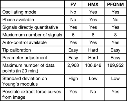
Table 1 Comparison of FV, HMX, and PFT modes in terms of available information, resolution, and ease-of-use.
Discussion
In the nineties, with the development of tapping mode [Reference Zhong9], most AFM operators used to refer to phase images as a simple way to show differences in mechanical or chemical properties between two components of the same sample [Reference Berquand10]. The phase image represents the energy dissipated between the tip and the sample during each tap on the surface and usually represents several factors that cannot be individually extracted. Unlike HMX and PFT, FV is not an oscillating technique. Among these three techniques, HMX is the only one directly based on the same principle as the tapping mode and thus the only one enabling extraction of the phase signal.
Quantitative measurements
In these three modes, because the tip can be calibrated prior to the experiment, the signals can directly be displayed in a quantitative manner. In FV, up to 6 signals can be simultaneously collected, including the height, the stiffness, the Young's modulus, and the adhesion. In
HMX and PFT, up to 8 channels can be displayed, including the same signals as in FV, as well as the peak force, the deformation, and the dissipation. Moreover, for these three modes, at least two different fit models can be used to calculate the Young's modulus in real time. In FV, the ramp rate as well as positive or negative triggers can easily be modulated. Also surface and retraction delays can be applied to control the interaction time between the tip and the surface. In HMX and PFT, the normal force applied to the sample is controlled by the applied set point. In HMX, the drive frequency can be manually modified but is usually fixed to a certain value (around 1 kHz) in PFT, although the latest instruments allow lowering this frequency to 0.5 or to 0.24 kHz. In terms of auto-control, FV imaging can be improved by z-closed loops, and the plots can automatically be centered during imaging. These features make FV imaging much more stable over time. The HMX and PFT modes, in addition to regular feedback control, can be combined with features like feedforward control [Reference Dickerson and Book11]. A feedback control system is always required to track set point changes and remove unmeasured disturbances that are present in any AFM image, but feedforward control can be enabled to suppress feed flow rate disturbances and automatically improve the quality of the imaging.
Calibration
Tip calibration and parameter adjustment are quite straightforward in FV and PFT but more challenging in HMX. Some HMX cantilevers exhibit overtones and often show a crosstalk between vertical and torsional signals, leading to artifact peaks. One major difficulty consists in finding the right torsional peak. In air, and for HMX-probes, this peak is usually found at 14 times the resonance frequency, but finding it in liquid is much harder and requires several attempts. Also, as in tapping mode, one has to adjust the drive frequency to avoid operating in unstable regimes (attractive-repulsive instabilities). This requires tuning far above the resonance (usually the peak offset has to be adjusted to 15%, instead of the usual 5% in tapping mode). As a comparison, PFT mode doesn't require any tuning or frequency adjustment. Moreover, in HMX, improving the signal-to-noise ratio often requires elimination of some of the first harmonics.
Image capture
Because they are based on different principles, FV, HMX, and PFT deliver different information and allow imaging at different resolutions. In our case, for an average capture time of 20 minutes and an image size of about 100 urn2, the resolution was about 3000, 100,000, and 200,000 pixels for FV, HMX, and PFT, respectively. Although an average Young's modulus could be calculated with the three techniques, the standard deviations were much higher with FV than with HMX and PFT images. This is mainly due to the fact that in similar operating conditions, FV provides approximately 30 to 70 fewer data points than HMX and PFT, respectively. Finally, in the case of FV and PFT images, the force curves can be extracted directly from the captured images and exported. This gives the user the possibility of using an external program to post-process the curves, by using various and customized algorithms to find the contact point, select a specific contact fit model, and calculate the Young's modulus. This option is disabled in HMX mode.
Conclusion
The FV, HMX, and PFT modes of AFM examined here exhibit different features. Image resolutions are typically 3,000, 100,000, and 200,000 pixels, respectively. Although all three modes can provide the average Young's modulus, the precision of this measurement is less with the FV mode. Also for FV and PFT, force curves can be extracted directly from the captured images. Thus, PFT appears as the best compromise between ease-of-use, acquisition speed, resolution, and amount of delivered information.
Acknowledgments
We would like to thank Andre Dabrunz and Ralf Schulz from University of Koblenz-Landau for providing the samples and for their technical input.