


1. Introduction
The main goal of hydrodynamic stability theory is to predict the parameters for which a given laminar flow can lose its stability and, possibly, turn turbulent. It requires monitoring both the short-time and long-time fate of infinitesimal disturbances to the so-called base flow (Schmid & Henningson Reference Schmid and Henningson2001). The concept of energy stability threshold is a key element of the associated toolbox. It refers to the largest value of the governing parameter (here the Reynolds number) below which the kinetic energy of all disturbances decays monotonically in time, regardless of their amplitude. For many academical flow cases, the value of that threshold, denoted  $Re_E$, matches exactly the value above which unstable modes are found. For flows characterised by strong non-normality of the associated linear operator, however, $Re_E$ lies strictly below the onset of instability. Such flows include most incompressible flows dominated by shear. Rather than separating stable from unstable regimes, it divides the real $Re$ axis into a lower range ( $Re \leqslant Re_E$) where all disturbances monotonically decay, and an upper range ( $Re > Re_E$) where energy growth is momentarily possible, possibly transient, at least for well-chosen initial conditions. Early historical examples of energy stability calculations include the works of Joseph, Busse and co-authors in simple subcritical flow configurations such as plane Couette flow, plane Poiseuille flow or pipe flow (Busse Reference Busse1969, Reference Busse1972; Joseph & Carmi Reference Joseph and Carmi1969; Joseph Reference Joseph1971), which have been revised recently (Falsaperla, Giacobbe & Mulone Reference Falsaperla, Giacobbe and Mulone2019; Xiong & Chen Reference Xiong and Chen2019; Nagy Reference Nagy2022). The transition to turbulence in such flows is known to be subcritical in Reynolds number, and to be dominated by linear yet non-normal effects (Reddy & Henningson Reference Reddy and Henningson1993; Trefethen et al. Reference Trefethen, Trefethen, Reddy and Driscoll1993). Since the exact transition threshold for actual subcritical transition is statistical it is typically difficult to evaluate (Lemoult et al. Reference Lemoult, Shi, Avila, Jalikop, Avila and Hof2016; Kashyap, Duguet & Dauchot Reference Kashyap, Duguet and Dauchot2022). The value of $Re_E$ given by energy stability theory appears as a much simpler quantity to evaluate in practice, since it is based mostly on linear mechanisms and is perfectly well-defined mathematically speaking.
Energy stability remains an important robustness indicator also for stable flow regimes, as it indicates a safe range of Reynolds numbers in which the flow can be operated without any risk of transition. Additional forces acting on a given flow affect the momentum and the energy balance, which can have a quantitative repercussion on the value of  $Re_E$. We focus in this paper on flows of liquid metals in channels and ducts in the presence of an imposed magnetic field. While this configuration is relevant for certain applications such as liquid metal cooling systems for fusion reactors (Müller & Bühler Reference Müller and Bühler2001), it remains a simplified configuration that is of fundamental interest in magnetohydrodynamic (MHD) research since the beginning of the field (Hartmann & Lazarus Reference Hartmann and Lazarus1937). For the parameters under study, the magnetic Reynolds number $Re_m$ is small enough so that the classical low- $Re_m$ approximation (Müller & Bühler Reference Müller and Bühler2001) holds, and no induction equation needs be taken into account. The magnetic field, depending on its orientation, generates Lorentz forces inside the flow that can modify the net force balance, while the presence of an electrical current contributes to increased dissipation. In particular, the global stability of the laminar flow can be enhanced if all velocity perturbations are damped by magnetic effects. This results in transition being delayed to higher Reynolds numbers, a property easily quantified by monitoring $Re_E$ (although the value of $Re_E$ underestimates in this case the exact values of $Re$ where transition occurs).
Specifically, the MHD duct accommodates two different types of boundary layers, namely the Hartmann and the Shercliff layers (Knaepen & Moreau Reference Knaepen and Moreau2008). These are respectively orthogonal and parallel to the applied magnetic field. For a unidirectional fluid flow subject to an externally imposed magnetic field, the interaction between the fluid motion and the magnetic field imposes a difference in electric potential between the Shercliff walls that drives a transversal electric current density. Assuming that the walls are electrically insulating, conservation of charge makes this current turn and reverse through the Hartmann layers such that closed current streamlines are formed. Due to such a reversal in the flow of charges, the Lorentz force, which is proportional to the current, tends to impede the fluid motion in the bulk and simultaneously accelerate the flow within the Hartmann layers (Müller & Bühler Reference Müller and Bühler2001). This in turn leads to Hartmann and Shercliff layers with different thicknesses: for the former, it is inversely proportional to the strength of the magnetic field, while for the latter, it is inversely proportional to its square root.
A large body of literature has already focused on the effects of a steady magnetic field imposed on a shear flow near rigid walls. The most dramatic consequence of the magnetic field is, when it is strong enough, an effective or quasi-two dimensionalization of the flow (Moreau Reference Moreau1990; Pothérat, Sommeria & Moreau Reference Pothérat, Sommeria and Moreau2000). This is expected and observed in practice outside boundary layers once the interaction parameter, which characterizes the ratio of Lorentz to inertial forces, becomes large compared with unity. For weaker magnetic fields, turbulent and transitional shear flows typically feature coherent structures such as streamwise streaks, like their non-MHD counterpart, but their range of existence in terms of  $Re$ differs. Nevertheless, from the point of view of transition to turbulence, they remain subcritical so that again a mismatch between the energy stability threshold $Re_E$ and the proper transition values is expected. Moreover, as in other shear flows, the underlying non-normality is strong, which results in strong amplification by transient growth mechanisms even without any instability of the base flow.
Most energy stability calculations have been done for very simple flow geometries. The earliest calculations were performed in plane channel geometries for planar Couette and Poiseuille flow (Joseph & Carmi Reference Joseph and Carmi1969). In the context of MHD flows amenable to the low- $Re_m$ approximation, the energy stability of the Hartmann layer has been studied by Lingwood & Alboussière (Reference Lingwood and Alboussière1999). Idealized geometries such as channel and boundary layer are never found neither in nature nor even in industrial contexts. We therefore decided to investigate the more realistic rectangular duct geometry, when the applied magnetic field is parallel to one of the sidewalls. This flow has been the subject of several experimental (Hartmann & Lazarus Reference Hartmann and Lazarus1937; Murgatroyd Reference Murgatroyd1953; Moresco & Alboussière Reference Moresco and Alboussière2004) and numerical studies (Kobayashi Reference Kobayashi2008; Krasnov et al. Reference Krasnov, Zikanov, Rossi and Boeck2010; Krasnov, Zikanov & Boeck Reference Krasnov, Zikanov and Boeck2012; Krasnov et al. Reference Krasnov, Thess, Boeck, Zhao and Zikanov2013; Zikanov et al. Reference Zikanov, Krasnov, Li, Boeck and Thess2014; Krasnov, Zikanov & Boeck Reference Krasnov, Zikanov and Boeck2015). Yet to our knowledge it has never been documented from the point of view of energy stability.
Duct geometries have long been used as research laboratories for the generalization of linear/nonlinear concepts first developed in channel geometries. In the context of transitional flows, instability threshold (Tatsumi & Yoshimura Reference Tatsumi and Yoshimura1990; Tagawa Reference Tagawa2019) transient growth (Krasnov et al. Reference Krasnov, Zikanov, Rossi and Boeck2010; Cassells et al. Reference Cassells, Vo, Pothérat and Sheard2019), edge states (Biau, Soueid & Bottaro Reference Biau, Soueid and Bottaro2008; Brynjell-Rahkola, Duguet & Boeck Reference Brynjell-Rahkola, Duguet and Boeck2022) and exact coherent states (Wedin, Bottaro & Nagata Reference Wedin, Bottaro and Nagata2009; Uhlmann, Kawahara & Pinelli Reference Uhlmann, Kawahara and Pinelli2010) have been recently documented in square duct geometries.
The goal of the present paper is to estimate numerically and report values of  $Re_E$ for rectangular ducts as functions of both the aspect ratio and the intensity of the magnetic field. The asymptotic cases of three-dimensional MHD channel flow are considered, as well as the quasi-two dimensional limit corresponding to strong magnetic fields. Besides this exhaustive parametric study, this study also aims at characterizing the coherent structures reported for these parameters, their symmetries, their link with linear optimal modes and their implication for transition to turbulence at higher Reynolds number.
The paper is structured as follows. The mathematical formulation of the continuous problem is given in § 2, together with the details about the numerical techniques (see also Appendix A). Results relevant to the channel geometry are first given in § 3. Duct results are shown in § 4. The description of optimal coherent structures is left for § 5. Conclusions and outlooks are given in § 6.
2. Problem formulation
Our aim is to model the flow of liquid metal in a periodic duct geometry with four sidewalls. The flow is subject to a magnetic field imposed in a direction transverse to the flow and parallel to one of the walls. For simplicity, we focus on the case where the walls are all electrically insulating.
2.1. Governing equations
The flow is governed by the incompressible Navier–Stokes equations for the velocity field, coupled to the Maxwell's equations for the magnetic part. The quasistatic approximation holds if the magnetic Reynolds number  $Re_m$ is negligible with respect to unity, which will be assumed throughout the whole paper. In this low- $Re_m$ approximation (Müller & Bühler Reference Müller and Bühler2001) the induced electric field can be represented as the gradient of the electric potential, determined by Ohm's law for a moving conductor in combination with Ampère's law, which requires the induced current density to be solenoidal. The original coupled system of equations reads
 $$\begin{gather} \frac{\partial \boldsymbol{u}}{\partial t} + (\boldsymbol{u} \boldsymbol{\cdot}\boldsymbol{\nabla})\boldsymbol{u} ={-} {\boldsymbol{\nabla} p} + \frac{1}{Re} {\nabla}^2 \boldsymbol{u} + \frac{Ha^2}{Re} \left(\kern2pt\boldsymbol{j}\times \boldsymbol{e}_B\right), \end{gather}$$
 $$\begin{gather}\boldsymbol{\nabla}\boldsymbol{\cdot} \boldsymbol{u}= 0, \end{gather}$$
 $$\begin{gather}\boldsymbol{j}={-}\boldsymbol{\nabla} \phi + \boldsymbol{u} \times \boldsymbol{e}_B, \end{gather}$$
 $$\begin{gather}\boldsymbol{\nabla}\boldsymbol{\cdot}\boldsymbol{j} =0 \leftrightarrow \nabla^2{\phi} = \boldsymbol{\nabla}\boldsymbol{\cdot} ({\boldsymbol{u} \times \boldsymbol{e}_B}). \end{gather}$$
The variables  $p$ and $\phi$ denote the pressure and electric potential, respectively, whereas ${\boldsymbol {u}}$ denotes the velocity field, $\boldsymbol {e}_B$ is the direction of the magnetic field and ${\boldsymbol {j}}$ the electric current density. All quantities are non-dimensionalized using the centreline velocity $U_{c}$ of the laminar flow for velocities, the shorter half-width $H$ of the duct for lengths, the strength $B_0$ of the imposed magnetic field and the electrical conductivity $\sigma$ of the fluid. This leads to a division by $\rho U_c^2$ for the pressure, by $U_cB_0H$ for the electric potential and by $\sigma U_cB_0$ for the electric current density. The governing non-dimensional control parameters are the Reynolds number
 \begin{equation} Re \equiv \frac{U_c H}{\nu} \end{equation}
and the Hartmann number
 \begin{equation} Ha \equiv B_0 H\sqrt{\frac{\sigma}{\rho\nu}}, \end{equation}
where  $\rho$ is the fluid density and $\nu$ is its kinematic viscosity. The walls are electrically insulating, i.e. the wall-normal component of the electric current density is zero at each wall. Besides the no-slip condition ${\boldsymbol {u}}={\boldsymbol {0}}$ is applied at each wall.
For the energy stability analysis, the flow is first decomposed, according to  ${\boldsymbol {u}}={\boldsymbol {U}} + {\boldsymbol {u}}'$, into the base laminar state with parallel velocity field $\boldsymbol {U}$ and a perturbation velocity field $\boldsymbol {u}'$. Moreover, a similar decomposition leads to the perturbation current density ${\boldsymbol {j}}'$, the perturbation electric potential $\phi '$ and the perturbation pressure $p'$. The equations for the perturbation fields $\boldsymbol {u}'$, $\phi '$ and $p'$ are
 $$\begin{gather} \frac{\partial \boldsymbol{u}'}{\partial t} \,{+}\, (\boldsymbol{U} \boldsymbol{\cdot} \boldsymbol{\nabla})\boldsymbol{u}' \,{+}\, (\boldsymbol{u}' \boldsymbol{\cdot}\boldsymbol{\nabla})\boldsymbol{U}+(\boldsymbol{u}' \boldsymbol{\cdot} \boldsymbol{\nabla})\boldsymbol{u}' \,{=}\,{-} {\boldsymbol{\nabla} p}' \,{+}\, \frac{1}{Re} {\nabla}^2 \boldsymbol{u}' \,{+}\, \frac{Ha^2}{Re} \left(\kern2pt\boldsymbol{j}'\times \boldsymbol{e}_B\right), \end{gather}$$
 $$\begin{gather}\boldsymbol{\nabla} \boldsymbol{\cdot} \boldsymbol{u}'= 0, \end{gather}$$
 $$\begin{gather}\boldsymbol{j}'={-}\boldsymbol{\nabla} \phi' + \boldsymbol{u}' \times \boldsymbol{e}_B, \end{gather}$$
 $$\begin{gather}\nabla^2{\phi}' = \boldsymbol{\nabla}\boldsymbol{\cdot} ({ \boldsymbol{u}' \times \boldsymbol{e}_B}), \end{gather}$$
where the boundary conditions for  $\boldsymbol {u}'$ are of Dirichlet type except at the inlet and outlet where periodicity is imposed. Superscript primes will be dropped from the perturbation quantities throughout the rest of this paper.
2.2. Duct and channel geometries
The main geometry under consideration in this study is a duct aligned with the streamwise direction  ${\boldsymbol {x}}$. The sides of the cross-section are parallel to the transverse directions ${\boldsymbol {y}}$ and ${\boldsymbol {z}}$. By convention, the magnetic field is aligned with the ${\boldsymbol {z}}$ direction, $\boldsymbol {e}_B=\boldsymbol {e}_z$ (this renders the coordinates $y$ and $z$ equivalent in the absence of the magnetic field). The velocity field is considered periodic in the streamwise direction with a period $L_x$. The distance between the sidewalls is noted as $2 L_y$ and $2 L_z$ in the $y$ and $z$ directions, respectively. The reference length $H$, used to build, for instance, the Reynolds number and the Hartmann number, is always taken to be half the shorter side of the cross-section. The pedagogic sketch in figure 1 explains how the geometry of the cross-section changes from $\gamma <1$ to $\gamma >1$, with $\gamma =1$ referring to a square duct.

Figure 1. Sketch of the geometry of a cross-section of duct flow, as the aspect ratio  $\gamma =L_y/L_z$ is varied from below to above unity ( $\gamma =1$ for a square duct). The labels $H$ and $S$ stand respectively for the Hartmann and Shercliff layers in the presence of a magnetic field aligned with the $z$ direction also noted ${\boldsymbol {e}}_B$. The reference length (used e.g. in the definition of the Hartmann number) is always one half of the shorter side: for $\gamma <1$ it is half of the distance between the Shercliff walls and for $\gamma >1$ it is half of the distance between the Hartmann walls. The channel case corresponds to the limit $\gamma \rightarrow 0$.
For the channel geometry, periodicity is assumed both in the streamwise and spanwise direction, which is called here  $y$. The reference length becomes the gap between the two walls, while the reference velocity $U_c$ is still the laminar centreline velocity.
2.3. Base flow
The base flow is streamwise independent and only the streamwise velocity component is non-zero. The induced current density is therefore two dimensional and can be represented by the induced streamwise magnetic field through Ampère's law,  $\boldsymbol {J}=\boldsymbol {\nabla }\times (B\boldsymbol {e}_x)$. The governing equations in dimensional form are
 $$\begin{gather} \varrho \nu \nabla^2 U + \frac{B_0}{\mu_0}\frac{\partial B}{\partial z} =\frac{\partial p}{\partial x}, \end{gather}$$
 $$\begin{gather}\lambda_m \nabla^2 B + B_0\,\frac{\partial U}{\partial z}= 0, \end{gather}$$
where  $\mu _0$ is the magnetic permeability of free space and $\lambda _m =1/(\mu _0\sigma )$ is the magnetic diffusivity. The gradient operators have to be understood as two-dimensional gradients defined with respect to the cross-flow variables $y$ and $z$ only. By choosing the shorter edge as the length scale and appropriate units for $U$ and $B$, one can make the prefactors of the terms multiplying the $z$ derivatives on the left-hand sides equal and the pressure gradient equal to unity. The non-dimensional equations for the base flow then read
 $$\begin{gather} \nabla^2 U + Ha\, \frac{\partial B}{\partial z} =1, \end{gather}$$
 $$\begin{gather}\nabla^2 B + Ha\, \frac{\partial U}{\partial z} =0. \end{gather}$$
These equations can be decoupled by adding and subtracting them. One obtains the two equations
 \begin{equation} \left(\nabla^2\pm Ha\,\frac{\partial }{\partial z}\right) \left(U\pm B\right)=1 \end{equation}
for the Shercliff variables  $U\pm B$ with homogeneous Dirichlet conditions.
An analytical solution to (2.15) in the form of a Fourier series was originally derived by Shercliff (Reference Shercliff1953) and later elaborated upon in Müller & Bühler (Reference Müller and Bühler2001). However, in this work (2.15) is discretized as described in § 2.6 and solved directly. Upon resolution, the desired base velocity distribution is obtained from the sum of the appropriately scaled Shercliff variables. This solution is shown in figures 2 and 3 for different duct aspect ratio  $\gamma$ and Hartmann numbers. The Hartmann and Shercliff layers on the walls $z=\pm 1$ and $y=\pm \gamma$ are clearly apparent by comparison between the cases ${{Ha}}=0$ and ${{Ha}}=20$.

Figure 2. Base flow for  ${{Ha}}=0$ (a,c) and ${{Ha}}=20$ (b,d) for an aspect ratio $\gamma =$1 (a,b) and $\gamma =2$ (c,d). Surface plot of the streamwise velocity $U(y,z)$.

Figure 3. Profiles of the base flow in the midplanes for different Hartmann numbers and  $\gamma =1$. (a) The $z$ profile of the streamwise velocity, (b) $y$ profile of the streamwise velocity, (c) $z$ profile of the streamwise magnetic flux density.
2.4. Energy stability as a minimization problem
Energy stability analysis is concerned with the behaviour of the total perturbation kinetic energy, defined as
 \begin{equation} E = \int_V \frac{u_i^2}{2} \, {\rm d}V, \end{equation}
using tensor notation. The evolution equation for  $E$ is obtained by multiplying the momentum equation (2.7) by $\boldsymbol {u}$ and integrating over the volume of the duct. Using integration by parts, this leads to
 \begin{equation} \frac{\partial E}{\partial t} ={-}\int_V u_i u_l \frac{\partial U_i}{\partial x_l} \, {\rm d}V- \frac{1}{Re} \int_V \frac{\partial u_i}{\partial x_l} \frac{\partial u_i}{\partial x_l}\, {\rm d}V - \frac{Ha^2}{Re}\int_V j_ij_i \, {\rm d}V. \end{equation}
This equation is equivalent to the Reynolds–Orr equation (Reddy & Henningson Reference Reddy and Henningson1993) in wall-bounded shear flows, save for the additional contribution of the Lorentz force. The slowest possible temporal decay of  $E$ occurs for the perturbation that provides the minimum of the functional (Doering & Gibbon Reference Doering and Gibbon1995)
 \begin{equation} \frac{1}{E} \left(\int_V u_i u_l \frac{\partial U_i}{\partial x_l} \, {\rm d}V+ \frac{1}{Re} \int_V \frac{\partial u_i}{\partial x_l} \frac{\partial u_i}{\partial x_l}\, {\rm d}V + \frac{Ha^2}{Re}\int_V j_ij_i \, {\rm d}V\right). \end{equation}
This functional is subject to the constraint (2.8), and the current density is represented by (2.9) and (2.10). We use Lagrange multipliers  $q$ and $\lambda$ to add the mass conservation and energy normalization constraints to the functional, i.e. we seek the extrema of the scalar functional $F$, defined by
 \begin{align} F &= \int_V u_i u_l \frac{\partial U_i}{\partial x_l} \, {\rm d}V+ \frac{1}{Re} \int_V \frac{\partial u_i}{\partial x_l} \frac{\partial u_i}{\partial x_l}\, {\rm d}V + \frac{Ha^2}{Re}\int_V j_ij_i \, {\rm d}V \nonumber\\ &\quad - \int_V q\, \boldsymbol{\nabla} \boldsymbol{\cdot} \boldsymbol{u}\, {\rm d}V -\lambda \left(E -1\right), \end{align}
where the minimization is carried over all admissible divergence-free velocity fields satisfying the boundary conditions. The current density  $\boldsymbol {j}$ depends directly on ${\boldsymbol {u}}$ and is given by (2.9) with $\phi$ satisfying (2.10). One stationarity condition is obtained via variation of the velocity field, i.e. from
 \begin{equation} 0=\frac{\delta F}{\delta \boldsymbol{u}}=\frac{{\rm d}}{{\rm d}\varepsilon}\left. F[\boldsymbol{u}+\varepsilon \delta \boldsymbol{u}]\right|_{\varepsilon=0}. \end{equation}
It leads to the Euler–Lagrange equation
 \begin{equation} \lambda \boldsymbol{u} ={+}\boldsymbol{\nabla} q + 2 \boldsymbol{\hat{S}} \boldsymbol{u} - \frac{2}{Re} \nabla^2 \boldsymbol{u} - \frac{2 Ha^2}{Re} \boldsymbol{j}\times \boldsymbol{e}_B, \end{equation}
where  $\boldsymbol {\hat {S}}$ is the symmetric part of the velocity gradient of the base flow and the current density is defined through (2.9)–(2.10). Variation of $F$ with respect to $q$ gives the constraint (2.8). The multiplier $\lambda$ is the growth rate of the perturbation satisfying (2.21), (2.8), (2.9) and (2.10) for given values $Re$ and ${{Ha}}$. We are interested in the lowest value of $Re$ where non-decaying solutions exist, i.e. $\lambda =0$. The minimizing velocity field is such that (2.21) reduces to the following eigenvalue problem for $Re$ (Doering & Gibbon Reference Doering and Gibbon1995):
 \begin{equation} Re\, \boldsymbol{\hat{S}} \boldsymbol{u} =-Re\frac{\boldsymbol{\nabla} q}{2} + \nabla^2 \boldsymbol{u} + Ha^2 \boldsymbol{j}\times \boldsymbol{e}_B. \end{equation}
The lowest eigenvalue  $Re$ defines the energy stability Reynolds number $Re_E$. The corresponding eigenvector represents a flow field whose kinetic energy does, for ${Re= Re_E}$, neither experience initial growth nor initial decay. The spectral problem (2.22) admits other eigenvalues beyond the lowest one. They correspond to larger values of $Re$ for which the problem admits neutral modes, i.e. non-monotonically decaying energy variations. By convention, each eigenvector indexed by $i=1,2,\ldots$ corresponds to the neutral flow field expressed at the value of $Re=Re^{(i=1,2,\ldots )}$.
2.5. Detailed formulation
The incompressiblity condition leads to difficulties for the numerical solution of the energy stability equations. We therefore adopt the approach used by Priede, Aleksandrova & Molokov (Reference Priede, Aleksandrova and Molokov2010) and represent the velocity field by a vector streamfunction  $\boldsymbol {\psi }$, i.e.
 \begin{equation} \boldsymbol{u}=\boldsymbol{\nabla} \times \boldsymbol{\psi}. \end{equation}
By that,  $\boldsymbol {\nabla }\boldsymbol {\cdot }\boldsymbol {u}=0$ is always satisfied. The vector streamfunction is defined only up to an additive gradient field. In order to fix this gradient field, we impose the gauge condition
 \begin{equation} \boldsymbol{\nabla}\boldsymbol{\cdot}\boldsymbol{\psi}=0, \end{equation}
whereby  $\boldsymbol {\psi }$ is defined up to the gradient of a harmonic function. The condition (2.24) also simplifies the relation between $\boldsymbol {\psi }$ and the vorticity field to $\boldsymbol {\omega }=-\nabla ^2\boldsymbol {\psi }$.
By taking the curl of (2.22), we obtain equations for  $\omega _y$ and $\omega _z$ and eliminate the field $q$. They read
 $$\begin{gather} \nabla^2 \omega_y -Ha^2 \frac{\partial }{\partial z}\left(\frac{\partial \phi}{\partial y}+u_x\right) = Re\, \boldsymbol{e}_y\boldsymbol{\cdot}\boldsymbol{\nabla}\times \boldsymbol{\hat{S}} \boldsymbol{u}, \end{gather}$$
 $$\begin{gather}\nabla^2 \omega_z -Ha^2 \frac{\partial^2 \phi}{\partial z^2} = Re\, \boldsymbol{e}_z\boldsymbol{\cdot}\boldsymbol{\nabla}\times \,\boldsymbol{\hat{S}} \boldsymbol{u}, \end{gather}$$
 $$\begin{gather}\nabla^2 \psi_y+ \omega_y = 0, \end{gather}$$
 $$\begin{gather}\nabla^2 \psi_z+ \omega_z = 0, \end{gather}$$
 $$\begin{gather}\nabla^2 \phi- \omega_z = 0. \end{gather}$$
2.5.1. Streamwise-dependent perturbations
Since the streamwise direction is homogeneous, the eigenfunctions of the energy stability eigenvalue problem are Fourier modes with streamwise wavenumber  $\alpha$. We therefore write
 \begin{equation} \left\{\boldsymbol{\psi},\boldsymbol{\omega},\phi\right\}(x,y,z)= \left\{\boldsymbol{\hat{\psi}}(y,z),\boldsymbol{\hat{\omega}}(y,z),\hat{\phi}(y,z)\right\}{\rm e}^{{\rm i}\alpha x}. \end{equation}
Equations (2.27)–(2.29) turn into three two-dimensional Helmholtz equations for each Fourier mode of the components  $\psi _y$, $\psi _z$ and the electric potential $\phi$ with the vorticity components as right-hand sides. Each of them is supplemented with a homogeneous boundary condition. Upon discretization, these equations become linear invertible mappings between the discrete representations of $\psi _y$, $\psi _z$ and $\phi$ and the discrete representations of $\omega _y$, $\omega _z$ augmented by a set of zero boundary data. The actual eigenvalue problem consists of (2.25)–(2.26) with $\omega _y$ and $\omega _z$ as independent variables. With this representation, the streamwise components $\psi _x$ and $\omega _x$ are directly obtained from the other two components $\psi _y, \psi _z$ and $\omega _y,\omega _z$ via (2.24) and $\boldsymbol {\nabla }\boldsymbol {\cdot }\boldsymbol {\omega }=0$.
The boundary conditions for the Fourier modes of  $\psi _y$, $\psi _z$ or $\omega _y$, $\omega _z$ have to be formulated such that the no-slip condition is satisfied. Following Priede et al. (Reference Priede, Aleksandrova and Molokov2010), we first impose that the tangential vector streamfunction component ${\psi }_t$ in the $(y,z)$ plane vanishes on each wall. This is admissible since it is equivalent to a Dirichlet condition for the arbitrary harmonic function (whose gradient can be added to $\boldsymbol {\psi }$). The other conditions are $u_x=0$ and $u_n=0$, where subscript $n$ denotes the normal component. We note that $u_n=0$ is equivalent to $\partial {\psi }_n/\partial n=0$ when ${\psi }_t=0$ and that $u_x=0$ implies $\partial {\psi }_z/\partial y-\partial {\psi }_y/\partial z=0$. The third condition $u_t=0$ in the $(y,z)$ plane is equivalent to $\omega _n=0$. For (2.27) for $\psi _y$ and (2.28) for $\psi _z$, one of the conditions $\psi _t=0$ and $\partial {\psi }_n/\partial n=0$ is selected on each segment of the boundary. Equation (2.29) for $\phi$ requires homogeneous Neumann conditions. Equations (2.25)–(2.26) are complemented with the conditions $\partial {\psi }_z/\partial y-\partial {\psi }_y/\partial z=0$ or $\omega _n=0$.
2.5.2. Streamwise-independent perturbations
The case of zero streamwise wavenumber must be treated separately since the representation of the streamwise velocity  $u_x$ by the other components fails when $\alpha =0$. One can then use the classical scalar streamfunction representation
 \begin{equation} u_y=\frac{\partial \psi_x}{\partial z}, \quad u_z={-}\frac{\partial \psi_x}{\partial y}, \end{equation}
for the in-plane components of the velocity. Likewise, the in-plane components of the electric current density are
 \begin{equation} j_y=\frac{\partial \chi}{\partial z}, \quad j_z={-}\frac{\partial \chi}{\partial y}, \end{equation}
where the streamfunction  $\chi$ for the current density is proportional to the streamwise component of the induced magnetic field. The streamwise current density is $j_x=u_y$. It stems from Ohm's law with the assumption that a mean streamwise current is excluded. Using Ohm's law one can also show that
 \begin{equation} \nabla^2 \chi={-}\frac{\partial u_x}{\partial z}. \end{equation}
Equations for  $\psi _x$, $\omega _x$, $u_x$ and $\chi$ are obtained from the streamwise component of (2.22) and the streamwise component of its curl. These equations are
 $$\begin{gather} \nabla^2 u_x + Ha^2 \frac{\partial \chi}{\partial z} = \frac{Re}{2} \left(\frac{\partial U}{\partial y}\frac{\partial \psi_x}{\partial z}- \frac{\partial U}{\partial z}\frac{\partial \psi_x}{\partial y}\right), \end{gather}$$
 $$\begin{gather}\nabla^2 \omega_x - Ha^2 \frac{\partial^2 \psi_x}{\partial z^2} = \frac{Re}{2} \left(\frac{\partial U}{\partial y}\frac{\partial u_x}{\partial z}- \frac{\partial U}{\partial z}\frac{\partial u_x}{\partial y}\right), \end{gather}$$
 $$\begin{gather}\nabla^2 \psi_x -\omega_x = 0, \end{gather}$$
 $$\begin{gather}\nabla^2 \chi + \frac{\partial u_x}{\partial z} = 0. \end{gather}$$
The boundary conditions for (2.36) and (2.37) are  $\psi _x=0$ and $\chi =0$. For the other two equations, the no-slip conditions $u_x=0$ and $u_t=0$ are required. The latter is equivalent to $\partial {\psi }_x/\partial n=0$. As discussed earlier for the case $\alpha >0$, the quantities $\chi$ and $\psi _x$ are obtained via one-to-one maps from $\omega _x$ and $u_x$. The actual eigenvalue problem consists of (2.34) and (2.35).
2.6. Spatial discretization for the duct and channel geometry
We use a spectral collocation method based on the Chebyshev polynomials  $T_0,T_1,\ldots$ defined over $[-1,1]$ by $T_n(x)=\cos (n\arccos x), n \geqslant 0$ (Canuto et al. Reference Canuto, Hussaini, Quarteroni and Zang2007).
For the duct flow, both cross-stream vorticity components are expanded as a finite double sum, i.e.
 \begin{equation} f(y,z)=\sum_{k=0}^{N_y}\sum_{l=0}^{N_z} \hat{f}_{k,l} T_k(y/L_y) T_l(z/L_z), \end{equation}
where  $f$ denotes either $\hat{\omega} _y$ or $\hat{\omega} _z$. Equations (2.25)–(2.26) and the corresponding boundary conditions for $\omega _y$, $\omega _z$ are enforced pointwise at the $(N_y+1)(N_z+1)$ Gauss–Lobatto collocation points $y_k$ and $z_l$ defined by
 \begin{equation} y_k=L_y\cos\left(k{\rm \pi}/N_y\right),\quad z_l=L_z\cos\left(l{\rm \pi}/N_z\right). \end{equation}
Each collocation point provides one scalar equation for the expansion coefficients of  $\omega _y$ and $\omega _z$ (Canuto et al. Reference Canuto, Hussaini, Quarteroni and Zang2007). The corners of the rectangular domain may require special consideration when derivatives are specified along the boundaries. In these cases it may be appropriate to impose the differential equation itself at a corner.
As a result, one obtains a generalized linear eigenvalue problem of the type
 \begin{equation} \boldsymbol{{{\boldsymbol{\mathsf{A}}}}} \boldsymbol{Y} =Re\, \boldsymbol{{{\boldsymbol{\mathsf{B}}}}} \boldsymbol{Y}, \end{equation}
where the vector  $\boldsymbol {Y}$ contains the unknown expansion coefficients of $\omega _y$ and $\omega _z$. The streamfunction components and the electric potential in (2.25)–(2.26) are represented as linear functions of $\omega _y$ or $\omega _z$ since they are given by (2.27)–(2.29). The discrete representation of these quantities is also obtained through spectral collocation. However, this requires more collocation points because $\psi _y$, $\psi _z$ and $\phi$ do not only depend on the inhomogeneity but also on the boundary data. We therefore use $(N_y+3)(N_z+3)$ expansion coefficients for $\psi _y$, $\psi _z$ and $\phi$ in the ansatz (2.38) and in (2.39a,b). By that, we obtain an invertible linear system between the expansion coefficients of either $\omega _y$ or $\omega _z$ augmented by the zero boundary data and the expansion coefficients of $\psi _y$, $\psi _z$ or $\phi$. These three inverse matrices are computed and stored before the matrices of problem (2.40) are assembled. The computation of these matrices as well as of matrices $\boldsymbol {{{\boldsymbol{\mathsf{A}}}}}$, $\boldsymbol {{{\boldsymbol{\mathsf{B}}}}}$ is described in the Appendix.
Problem (2.40) was solved with MATLAB's eig routine (The MathWorks, Inc. 2020) to find all eigenvalues and eigenvectors. The routine also works with a matrix  $\boldsymbol {{{\boldsymbol{\mathsf{B}}}}}$ whose rank is smaller than the rank of $\boldsymbol {{{\boldsymbol{\mathsf{A}}}}}$ (as it is the case for (2.40)). It associates the spurious solutions that stem from equations not containing the eigenvalue $Re$ with infinite eigenvalues. The numerical approach for the special case $\alpha =0$ is analogous with $\omega _x$ and $u_x$ taking the role of $\omega _y$ and $\omega _z$ as primary unknowns.
In contrast to the duct geometry, the base flow in the infinitely wide channel depends only on the  $z$ coordinate. Owing to this homogeneity, the solution to the eigenvalue problem can be represented by Fourier modes with respect to $x$ and $y$ with arbitrary wavenumbers $\alpha$ and $\beta$. The ansatz for a velocity or vorticity component then becomes
 \begin{equation} f(x,y,z)=\sum_{k=0}^{N_z} \tilde{f}_{k}\, T_k(z/L_z) \exp({{\rm i}( \alpha x +\beta y)}). \end{equation}
The velocity field is represented through the vertical velocity and vorticity components. Equations for these quantities are obtained by taking the vertical components of the curl and the double curl of the stability eigenvalue problem (2.22). These equations are complemented by (2.10) for the electric potential. The number of unknowns corresponds to the expansion coefficients of vertical velocity, vorticity and potential, i.e. approximately  $3 N_z$. The discretized form is obtained by enforcing the equations pointwise at collocation points $z_k$, and the resulting generalized linear eigenvalue problem, also of the form (2.40), is solved with MATLAB's eig routine. The energy stability of the quasi-two-dimensional (Q2D) model was formulated in a similar way with the spanwise velocity component as the sole dependent variable.
2.7. Code verification and numerical resolution
The code has previously been used in the context of magnetoconvection (Bhattacharya et al. Reference Bhattacharya, Boeck, Krasnov and Schumacher2024). Its accuracy for the duct geometry was verified with linear stability results from the hydrodynamic literature. For the streamwise-independent perturbations, we computed the eigenvalues of the Stokes operator for  $\gamma =1$ and compared them with Leriche & Labrosse (Reference Leriche and Labrosse2004). The 10 leading eigenvalues in table 2 of Leriche & Labrosse (Reference Leriche and Labrosse2004) were reproduced to at least eight significant digits with a resolution of $N_y=N_z=25$. For the perturbations with $\alpha >0$, we took a case from Priede et al. (Reference Priede, Aleksandrova and Molokov2010) (their table 2, left column) with a simplified base flow $(1-y^2)(1-z^2)$ in a square duct. For $Re=10^4$, $\alpha =1$, we reproduced the complex relative phase velocity of the leading eigenmode to six significant digits with a resolution of $N_y=N_z=60$ modes.
A direct comparison for energy stability was only possible without a magnetic field for  $\gamma =1$ (see § 4.1). The additional electromagnetic terms in the equations could not be checked directly. However, the MHD channel results should provide appropriate limits to the duct results for either large ${{Ha}}$ or small/large $\gamma$. This will also become apparent in the following sections.
The numerical resolution for the duct flow has to be increased with  ${{Ha}}$ in order to resolve the electromagnetic boundary layers. The requirements were systematically tested for $\gamma \approx 1$ and different ${{Ha}}$ by comparing two different resolutions. Table 1 indicates that the results are sufficiently accurate for the lower order $N_1$ of Chebyshev polynomials. However, the accuracy also depends on $\alpha$. It becomes poorer as $\alpha$ is decreased. This can be expected since $\alpha \to 0$ is a singular limit for the formulation based on $\omega _y$ and $\omega _z$.
Table 1. Resolution tests for MHD duct flow with  $\alpha =2$. Energy stability eigenvalues $Re_E$ were computed with maximum orders $N_1$ and $N_2$ of Chebyshev polynomials in both $y$ and $z$ resulting in a difference $\Delta Re_E$.

When the aspect ratio  $\gamma$ is not close to unity, the number of polynomials must be increased along the longer edge of the duct to maintain adequate resolution. We decided to keep the maximum spacing of the collocation points constant on the longer edge. Since this spacing scales as $1/N$ (where $N$ is the polynomial order), the appropriate choice is to multiply $N_y$ by $\gamma$ or to divide $N_z$ by $\gamma$ (for $\gamma >1$ and $\gamma <1$, respectively). This is done relative to the reference case $\gamma =1$. Depending on the lowest $\alpha$ of interest, the base resolution may have to be increased to ensure valid results. This can also be detected from the magnitude of the imaginary part of $Re_E$, which should ideally be zero. Eigenvalues with significant imaginary parts are discarded in the computations.
The numerical resolution is mainly limited by the computing time, which approximately scales with the third power of the number of unknowns. For  $N_y=N_z=60$, the assembly of the matrices and eigenvalue computation took about 2.5 hours for fixed $\alpha$ and $\gamma$ on an Intel Xeon E5 processor.
3. Channel geometry
3.1. Energy stability for  ${{Ha}}=0$

We begin by considering the purely hydrodynamic channel case with only two parallel walls, when  ${{Ha}}=0$. This configuration is one of the earliest cases treated in the literature. For a recent comparative review, we refer, for instance, to Falsaperla et al. (Reference Falsaperla, Giacobbe and Mulone2019). Orr has initially sought neutral modes under the hypothesis that their spanwise wavenumber $\beta$ is zero and found analytically a value of $Re_E\approx 87$ (Orr Reference Orr1907). A more accurate value is $Re_E= 87.6$ at $\alpha = 2.09$ (Falsaperla et al. Reference Falsaperla, Giacobbe and Mulone2019). Later Joseph & Carmi (Reference Joseph and Carmi1969), Busse (Reference Busse1969), by seeking neutral perturbations with zero streamwise wavenumber $\alpha$, reported a lower value of $Re_E= 49.6$ at $\beta = 2.04$. In the present computation, both $\alpha$ and $\beta$ can be freely varied. The two values of $Re_E$ put forward by Orr and by Busse (Reference Busse1969) are confirmed in figure 4 by focusing on the axes $\alpha =0$ or $\beta =0$. Whereas the value for $\alpha =0$ corresponds to a local minimum of $Re_E$ in the $(\alpha,\beta )$ plane, the minimizer for $\beta =0$ appears as a saddle in the unfolded $(\alpha,\beta )$ plane.

Figure 4. Cartography of  $Re_E$ in the $(\alpha,\beta )$ plane, where $\alpha$ and $\beta$ are the streamwise and spanwise wavenumbers, respectively. Channel geometry, from (a–d) ${{Ha}}=0,5,10,20$.
3.2. Influence of increasing ${{Ha}}$

The local minima of the  $Re_E$ in the $(\alpha,\beta )$ plane evolve as ${{Ha}}$ departs from zero. Maps of $Re_E$ can be seen in figure 4 for ${{Ha}}=5,10$ and $20$. For ${{Ha}} \geqslant 10$, the global minimizer for $Re_E$ corresponds to a mode with $\beta =0$ in strong contrast with the case ${{Ha}}=0$. This minimizer is actually independent of ${{Ha}}$ since there is no Lorentz force for $\beta =0$. It represents the solution found by Orr. For the intermediate value ${{Ha}}=5$, the minimizer is neither along the axis $\alpha =0$ nor along the axis $\beta =0$. Instead it corresponds to an oblique wave vector with both $\alpha$ and $\beta$ non-zero.
4. Rectangular duct geometry
We move now to the rectangular duct case with four walls and a transverse magnetic field parallel to one of the walls. The minimization problem leading to the value of  $Re_E$ is governed by two main parameters, notably the aspect ratio $\gamma =L_y/L_z$ and the Hartmann number ${{Ha}}$ based on the shorter edge.
4.1. Energy stability for ${{Ha}}=0$

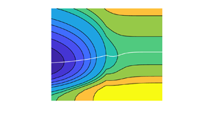
Figure 5 shows colour maps of the values of  $Re_E$ in an $(\alpha,\gamma )$ plane, where $\alpha$ is the streamwise wavenumber and $\gamma$ is represented in (base 10) logarithmic scale. Values of ${{Ha}}=0,5,10$ and $20$ are shown. The numerical resolutions for these computations are given in table 2.

Figure 5. Cartography of  $Re_E$ in the $(\alpha,\log _{10}(\gamma ))$ plane. Duct geometry, from (a–d) ${{Ha}}=0,5,10,20$.
Table 2. Resolutions for the computations of figure 5 indicated by maximum order of Chebyshev polynomials. The square brackets denote the integer part.

We focus first on figure 5(a) that has  ${{Ha}}=0$. As far as we know, no exhaustive energy stability study has been performed in a rectangular duct flow even in the absence of MHD effects. This configuration, where ${{Ha}}=0$, is characterized by an additional degree of symmetry compared with the MHD case: all sidewalls are equivalent and the notion of Shercliff and Hartmann walls is irrelevant. Mathematically this results in the equivalence between an aspect ratios $\gamma =L_y/L_z>0$ and its inverse $1/\gamma =L_z/L_y$. We thus expect the symmetric relation $Re_E(\gamma )=Re_E(1/\gamma )$ to be valid. This should manifest itself graphically in a flip symmetry with respect to the zero axis when plots are made according to the variable $\log {\gamma }$. As expected, the symmetry property $Re_E(\gamma )=Re_E(1/\gamma )$ is clearly visible in the figure.
The location of the wavenumber  $\alpha =\alpha _m$ associated with the optimal value $Re_E$ has been represented in figure 5 for each value of $\gamma$, by using a plain white line. For the case ${{Ha}}=0$, non-zero values of $\alpha _m$ appear to be restricted to an interval where $|\log _{10}(\gamma )| \lesssim 0.2$, i.e. $0.6 \lesssim \gamma \lesssim 1.6$. The largest value of $\alpha _m$ (i.e. the shortest wavelength) is found on the symmetry axis for $L_y=L_z$ and corresponds to the cusp in the figure. Outside this interval the wavenumber minimizing $Re_E$ is everywhere zero.
The variation of  $Re_E$ (at optimum wavenumber) with $\gamma$ is shown in figure 6(a). As one would expect, the values for ${{Ha}}=0$ approach the channel limit with $Re=49.6$ for decreasing as well as for increasing $\gamma$. One can also notice two discontinuities in the slope of the curve $Re_E(\gamma )$ on either side of $\gamma =1$. For $\gamma >1$, these occur at $\gamma \approx 1.8$ and $\gamma \approx 2.8$. They correspond to a qualitative change in the structure of the mode providing $Re_E$, which will be shown in § 5.

Figure 6. Plots of  $Re_E$ and $\alpha _m$ vs $\gamma$ in the duct geometry.
We focus now on the square case, i.e.  $\gamma =1$. In the literature, to our knowledge only a numerical value of $Re_E = 79.44$ (based on the centreline velocity) has been reported by Biau et al. (Reference Biau, Soueid and Bottaro2008) in the absence of MHD effects, associated with a zero streamwise wavenumber. This is at odds with our result $\alpha = 1.3$ corresponding to a smaller value $Re_E = 74.1$. For $\alpha =0$, we obtain $Re_E=78.5$ in reasonable agreement with Biau et al. (Reference Biau, Soueid and Bottaro2008), where a different numerical method was used. We note, for comparison, that the companion circular geometry of Hagen–Poiseuille flow also features a non-zero axial optimal wavenumber $\alpha =1.07$ found for $Re_E = 81.5$ (Joseph & Carmi Reference Joseph and Carmi1969).
4.2. Influence of increasing ${{Ha}}$

As  ${{Ha}}$ increases above zero, the flip symmetry in figure 5(a) is immediately lost. This corresponds to an increasing dissymmetry between the two different pairs of boundary layers along the sidewall: the Hartmann and the Shercliff boundary layers are now two distinct boundary layers with different scalings. The minimal value of $Re_E$ in figure 5 is always achieved, unlike for ${{Ha}} = 0$, for a finite wavenumber $\alpha _m$. This minimum is always found at the lowest $\gamma$ values computed. This corresponds to the configuration where the longer edge is parallel to the magnetic field: the laminar base flow is then dominated by wider Shercliff layers and the two thinner Hartmann layers are well separated. The minimal value of $Re_E$ itself increases with ${{Ha}}$. For ${{Ha}}=0,5,10,20$, it is respectively 52.2, 88.1, 102.2 and 127.3.
The global trend for the value of  $Re_E$ is an increase with ${{Ha}}$, which is also seen in figure 6(a). It appears that $Re_E$ and the corresponding wavenumber $\alpha$ shown in figure 6(b) approach Orr's value represented by a black square on the left axis $\gamma =0.25$ for all ${{Ha}}\geqslant 5$. This is consistent with the channel flow with a spanwise magnetic field because the base flow in the duct approaches the Poiseuille profile as $\gamma$ tends to zero (with the exception of the Hartmann layers).
Figures 6(a) and 6(b) also show that a plateau emerges for both  $Re_E$ and $\alpha _m$ at large $\gamma$. The higher the value of ${{Ha}}$, the earlier the plateau is reached as $\gamma$ is increased. For ${{Ha}} \geqslant 5$, $\alpha _m$ stays away from zero for all aspect ratios $\gamma$ shown. The range of values of $\alpha _m$ found by varying $\gamma$ shifts upwards as ${{Ha}}$ is increased. This corresponds, as ${{Ha}}$ gets larger, to increasingly shorter wavelengths found at criticality. For ${{Ha}}=10$ and beyond, the shorter wavelengths are found for $\gamma >1$.
4.3. Connection with the quasi two-dimensional theory
We investigate now the other limiting configuration  $\gamma \rightarrow \infty$ where the shorter edge is parallel to the magnetic field. This is associated visually with the right of each subplot in figure 5, in which the same values of ${{Ha}}=0,5,10$ and $20$ are displayed. In this configuration, the laminar flow consists of two narrow Shercliff layers and two laterally extended Hartmann layers. From figure 5 it is clear that, at least for ${{Ha}} \neq 0$, $Re_E$ achieves, for asymptotically large $\gamma$, a minimum value associated with non-zero values of $\alpha _m$. The corresponding values of $Re_E$ and $\alpha _m$ are reported in figures 7(a) and 7(b), respectively. The additional values of $Re_E$ and $\alpha _m$ for ${{Ha}}>20$ were typically computed at two distinct values of $\gamma >1$. This was done in order to ensure that the plateau is reached without going to the computationally expensive case $\gamma =4$.

Figure 7. Plots of (a)  $Re_E$ vs ${{Ha}}$, (b) $\alpha _m$ vs ${{Ha}}$ in the duct geometry (in the large $\gamma$ limit), with comparison with (4.1) from Q2D theory.
Both  $Re_E$ and $\alpha _m$ increase monotonically with increasing ${{Ha}}$. This is interpreted, for this large $\gamma$ limit, as a delay of the transition by the magnetic field, associated with smaller axial wavelengths at criticality.
The present results can be compared with earlier work (Pothérat Reference Pothérat2007) carried out in the framework of the Q2D approximation (Sommeria & Moreau Reference Sommeria and Moreau1982; Pothérat et al. Reference Pothérat, Sommeria and Moreau2000). In the Q2D model the flow is represented by a two-dimensional velocity field that corresponds to the actual flow averaged along the direction of the magnetic field. The averaged flow satisfies the two-dimensional Navier–Stokes equations with an additional linear damping term  $-{{Ha}}_{\rm {Q2D}} \boldsymbol {u}$. This term accounts for the friction on the Hartmann walls. The Q2D Reynolds number is defined with the lateral dimension $L_y/2$, i.e. $Re_{\rm {Q2D}} = \gamma Re$. Correspondingly, $\alpha _{\rm {Q2D}}=\alpha /\gamma$. The relation between ${{Ha}}_{\rm {Q2D}}$ and ${{Ha}}$ is ${{Ha}}_{\rm {Q2D}}= \gamma ^2 {{Ha}}/2$. The basic flow in the Q2D model is equivalent to the Hartmann flow profile but with a side layer thickness $\sim {{Ha}}_{\rm {Q2D}}^{-1/2}$. For ${{Ha}}_{\rm {Q2D}} \gg 1$, the Q2D energy stability analysis shows a universal, self-similar dependence between Reynolds and wavenumber illustrated in figure 8(a). This agreement between different ${{Ha}}_{\rm {Q2D}}$ demonstrates that the (averaged) Shercliff layers on the opposite walls become decoupled, i.e. outer length scale (width of the duct) does not affect the result. In particular, the minimum $\alpha _{\rm {Q2D}}$ and the corresponding $Re_{\rm {Q2D}}$ therefore scale as ${{Ha}}_{\rm {Q2D}}^{1/2}$. The numerical values of the coefficients in the scaling relations are given in Pothérat (Reference Pothérat2007). Transformed to our definitions, they read
 \begin{equation} Re= 65.3 \sqrt{Ha}, \quad \alpha=0.863\sqrt{Ha}. \end{equation}
The qualitative as well as quantitative match between the present computations and the Q2D results in figure 7 is good, despite a slight drift observed for the largest values of  ${{Ha}}$ (computed here up to $Ha=80$). The perturbations are therefore expected to become localized in the Shercliff layers, and to exhibit a shape with approximate uniformity along the magnetic field.

Figure 8. Plots of  $Re_E$ vs $\alpha$, with all quantities rescaled by their value at the minimum $Re_E$. (a) Rescaled results from the Q2D model for several ${{Ha}}_{\rm {Q2D}}$. (b) Comparison of duct results (in the limit $\gamma \gg 1$) with results from the Q2D model.
We can further verify the universal scaling behaviour for our duct results over intervals of  $\alpha$. This is reported in figure 8(b). It shows the dependence of normalized $Re_E$ and $\alpha$ for different ${{Ha}}$ as well as the universal curve from the Q2D model in figure 8(a). The agreement with the Q2D model is excellent except in the limit $\alpha \to 0$, where the duct curves depart from the Q2D theory. In contrast to the Q2D asymptotic behaviour $Re\sim 1/\alpha$, they saturate at finite values of $Re$ for $\alpha =0$. These values increase monotonically with ${{Ha}}$.
As already noted, the dependence  $Re(\alpha )$ in the Q2D model appears to be a power law for $\alpha \to 0$ and for $\alpha \to \infty$ (see figure 8a). The former is consistent with a regular limit $\alpha \to 0$ in the Q2D equations. The $O(\alpha ^2)$ scaling for large $\alpha$ cannot be justified in this way. It can be understood as a diffusive scaling associated with wavelengths with a viscous damping rate $O(\alpha ^2Re^{-1})$ so high that it requires $Re=O(\alpha ^2)$ for damping to be balanced instantaneously by non-normal amplification.
4.4. Case $\alpha =0$

While the disturbances with  $\alpha =0$ do not minimize $Re_E$ for ${{Ha}}\geqslant 5$, they are interesting in their own right since their corresponding $Re_E$ has a different dependence on ${{Ha}}$ than the optimal mode. This is apparent from figure 9(a) that shows the $\gamma$ dependence of $Re_E$ for $\alpha =\alpha _m$ and $\alpha =0$. For large $\gamma$, $Re_E$ for $\alpha =0$ saturates like the minimal $Re_E$ but the saturation levels for $\alpha _m$ and $\alpha =0$ separate further as ${{Ha}}$ grows. For small $\gamma$, a saturation is only apparent for ${{Ha}}=5$ with comparable levels for $\alpha _m$ and $\alpha =0$. For ${{Ha}}= 10$ and ${{Ha}}=20$, the curves for $\alpha _m$ and $\alpha =0$ continue to decay below $\gamma =0.25$. It can be expected that the curves for $\alpha =0$ eventually reach the saturation levels for the channel case. These correspond to the minima of $Re_E$ on the axis $\alpha =0$ in figures 4(c) and 4(d). For ${{Ha}}=10$ and ${{Ha}}=20$, these values are $Re_E\approx 158$ and $Re_E\approx 310$, respectively.

Figure 9. (a) Plot of  $Re_E$ for $\alpha =0$ (full lines) and optimal $\alpha$ (dashed) vs $\gamma$ in duct geometry. (b) Plot of $Re_E$ for $\alpha =0$ (duct, limit $\gamma \gg 1$) vs ${{Ha}}$ and comparison with Hartmann layer scaling.
The saturated values of  $Re_E$ for $\alpha =0$ and $\gamma >1$ are shown in figure 9(b) as black circles. They clearly scale as $Re_E\sim O({{Ha}})$ with a proportionality constant $\approx 23$. This linear scaling is consistent with the behaviour of linear, streamwise-independent optimal perturbations investigated by Krasnov et al. (Reference Krasnov, Zikanov, Rossi and Boeck2010). These authors found that those perturbations reside in the Shercliff layers. A linear scaling was also obtained by Lingwood & Alboussière (Reference Lingwood and Alboussière1999). These authors investigated energy stability for a single insulating Hartmann layer. They found $Re_E=25.6\, {{Ha}}$ for purely streamwise-independent modes ( $\alpha =0$). Although the numerical value of the proportionality constant for the duct is close to $25.6$, the corresponding modes are distinct. Perturbations localized in the Hartmann layers only appear as higher modes in the duct case. For $\gamma =1$, the ninth mode is the lowest one with such a spatial structure. The corresponding $Re_E$ of the ninth mode (also displayed in figure 9b) agrees very well with the energy stability limit from Lingwood & Alboussière (Reference Lingwood and Alboussière1999).
In summary, the case  $\alpha =0$ provides a linear dependence between Reynolds and Hartmann numbers for energy stability. This is consistent with threshold values of $Re$ found in experiments on the relaminarization of turbulent MHD duct flows (Branover Reference Branover1978; Moresco & Alboussière Reference Moresco and Alboussière2004). A scaling with ${{Ha}}^{1/2}$ is not observed in those experiments. This underlines the dynamical importance of long-wave modes in transitional and turbulent MHD duct flows despite their non-optimal properties.
5. Coherent structures at criticality
5.1. Theoretical link with linear optimal perturbations
Although many energy stability calculations principally report values of  $Re_E$ and the corresponding optimal wavenumbers at criticality (i.e. at $Re=Re_E$), the associated flow structures, corresponding to the eigenvectors of the linearized operator in (2.22), are usually not investigated in detail with the possible exception of Pothérat et al. (Reference Pothérat, Sommeria and Moreau2000). These coherent structures are not directly observable flow structures in an experimental setting, unlike, e.g. unstable global modes. However, as mentioned earlier, they bear a strong relation with the linear optimal perturbations (LOPs) celebrated in non-modal instability analysis (Schmid Reference Schmid2007; Kerswell Reference Kerswell2018). The LOPs are the initial velocity fields ${\boldsymbol {u}}^{(T)}_{opt}$ that optimize the finite-time perturbation energy growth
 \begin{equation} G(T,{\boldsymbol{u}}(0))=|{\boldsymbol{u}}(T)|^2/|{\boldsymbol{u}}(0)|^2 \end{equation}
for any given time horizon  $T>0$, under the action of the linearized dynamics (Reddy & Henningson Reference Reddy and Henningson1993). They are relevant for $Re>Re_E$, when energy growth is indeed instantaneously possible and $\max {(G)}>1$ for at least some value of $T$. The maximum energy growth corresponding to the short-time horizons $\Delta t \ll 1$ verifies $G(\Delta t,{\boldsymbol {u}}^{\Delta t}_{opt}) \leqslant \lVert \boldsymbol {\mathcal {I}}+2(\Delta t)\boldsymbol {\mathcal {L}} \rVert$ at first order in $\Delta t$, where $\boldsymbol {\mathcal {L}}$ is the linearized operator at $t=0$. This tends to unity, for fixed $\Delta t$, as $Re$ approaches $Re_E$ from above. The structures achieving the largest energy growth at $Re=Re_E$ are hence precisely the critical perturbations computed in all energy stability studies as a byproduct of the eigenvalue problem (2.22). In other words, the LOPs computable at $Re>Re_E$ continue smoothly into the critical perturbations computed here. In the same way as the detailed investigation of the LOPs has shed light on the (linear) transition mechanisms, it is hence useful to investigate the critical perturbations at $Re_E$ as they might already feature elements related to the transition observed at larger $Re$. This is, for instance, the case for the channel flow discussed in § 3, where the mode that attains the lowest $Re_E$ changes from a streamwise to a spanwise uniform structure as ${{Ha}}$ is increased and, for intermediate parameter values, corresponds to an oblique wave. Such a trend is in complete agreement with the behaviour of LOPs reported by Krasnov et al. (Reference Krasnov, Rossi, Zikanov and Boeck2008) (see their figure 7). On a technical level, the critical perturbations computed from (2.22) are independent of any target time, which makes their description simpler.
It is useful to recall the main teachings of the quest for LOPs in simple configurations, namely the purely hydrodynamic channel flow with streamwise periodicity. Two-dimensional computations (assuming no spanwise dependence of the flow) have highlighted the Orr mechanism as the most efficient way to extract energy from the base flow (Farrell Reference Farrell1988). The Orr mechanism consists of a progressive shearing of the perturbations in the direction associated with the base flow. The corresponding optimal perturbations are easily recognized by the tilting of spanwise vortices against the shear. Three-dimensional computations of LOPs have highlighted a much more efficient energy growth mechanism, linked to the lift-up mechanism (Brandt Reference Brandt2014) that actively exploits the spanwise dependence of the disturbance. The associated optimal perturbations look like long tubular streamwise vortices evolving rapidly into streamwise streaks, characterized by a well-defined spanwise spacing. These optimal disturbances are often two dimensional (Butler & Farrell Reference Butler and Farrell1992), now in the sense that they do not depend on the streamwise coordinate, and even when they are three dimensional, the tilting of the vortices against the shear is not pronounced.
5.2. Duct visualization for ${{Ha}}=0$

We begin by visualizing the eigenmodes of the eigenproblem (2.22) in the non-MHD case when  ${{Ha}}=0$. Starting with the least stable modes and focusing on the square duct ( $\gamma =1$), figure 10(a–c) shows three-dimensional rendering of the isosurfaces of $u_x$ for three values of $\alpha$ from low to high, respectively $\alpha =0.6,1.2$ and $2.4$. The tilting against the shear typical of Orr modes is found visually in figure 10. This tilting is confirmed by looking at the perturbations both in the $xy$ and $xz$ planes, as shown in figure 11 for the same values of $\alpha$.

Figure 10. Isosurfaces of  $u_x$ for the leading eigenmodes at ${{Ha}}=0$, $\gamma =1$ and streamwise wavenumbers (a) $\alpha =0.6$, (b) $\alpha =1.2$ and (c) $\alpha =2.4$. The streamwise period displayed in each case is the period for $\alpha =1.2$.

Figure 11. Contours of  $u_x$ in the planes $z=0$ (a–c) and $y=1/2$ (d–f) for the leading eigenmodes at ${{Ha}}=0$ for the same parameters as figure 10.
For a better visualization of the flow in a cross-section, we chose to display in figure 12 only the real part of the velocity field associated with  $u_x$, and chose (before normalization) the cross-section where the amplitude of ${Re}(u_x)$ is maximal. This representation makes the symmetries of the different modes easier to interpret. In particular, figure 12 shows the four least stable modes. We can adopt the nomenclature introduced in the linear stability analyses of Tatsumi & Yoshimura (Reference Tatsumi and Yoshimura1990) (for hydrodynamic duct flow) and Priede et al. (Reference Priede, Aleksandrova and Molokov2010) (for the Hunt's flow that admits the same symmetry classification), which is based on listing whether the symmetry of $u_x$ with respect to the $z$ axis (respectively the $y$ axis) is odd or even. It can be checked that this classification remains unaffected by the presence of the Lorentz force in the governing equations. This gives way to the respective symmetry types I (odd in $y$, even in $z$), II (odd in $y$ and $z$), III (even in $y$ and $z$) and IV (even in $y$, odd in $z$). The modes listed in figure 12 are (a) type IV, (b) type I, (c) type III and (d) type II.

Figure 12. Eigenmodes by ascending  $Re_E$ from (a–d) for ${{Ha}}=0$, $\gamma =1$ and $\alpha =0.3$ visualized by the real part of $u_x$. Here $u_x$ is normalized such that its maximum is equal to unity. These modes correspond to type I (b), type II (d), type III (c) and type IV (a).
The values of  $Re_E$ corresponding to each of these four modes are, for a more efficient representation, plotted versus their corresponding optimal wavenumber $\alpha$ in figure 13. It is clear that the two modes with symmetry types I and IV are equivalent for $\gamma =1$ and the optimal structure for all values of $\alpha$. Modes II and III cross near $\alpha =2$.

Figure 13. Plot of  $Re_E$ vs $\alpha$ for different modes computed for ${{Ha}}=0$, $\gamma =1$.
For  ${{Ha}}=0$, the structure and symmetry type of the lowest mode can change with the aspect ratio $\gamma$. This was already noted in connection with figure 6(a). The plots of cross-sections of $u_x$ for $\gamma =2$ and $\gamma =4$ are shown in figure 14. These modes have symmetry II. At $\gamma =4$, the number of structures along the $y$ direction is twice that for $\gamma =2$.

Figure 14. Lowest eigenmodes (type II) for  ${{Ha}}=0$, $\alpha =0$ and (a) $\gamma =2$, (b) $\gamma =4$ visualized by $u_x$. Here $u_x$ is normalized such that its maximum is equal to unity.
5.3. Duct visualization for ${{Ha}} \neq 0$

We move next to the visualization of the eigenmodes of the eigenproblem (2.22) in the MHD case. Figure 15 shows three-dimensional visualizations of the least stable modes found in square duct ( $\gamma =1$) at ${{Ha}}=20$ for $\alpha =1/2,1,2$ and $4$. Again, long modes with small or vanishing $\alpha$ are associated at higher $Re$ with the lift-up mechanism while the Orr mechanism is present in shorter-wavelength structures. A clear difference is that the structures are more localized near the sidewalls since the central part of the velocity distribution has low shear. As for ${{Ha}}=0$, the streamwise velocity has also been plotted in the $xy$ plane where variations along $y$ are important (see figure 16), whereas in the $xz$ plane the perturbations show a more uniform dependence on $z$. The tilting against the shear, clearly visible in the Shercliff layers, is noted for $\alpha =1,2$ as well as for $\alpha =4$ where the lowest value of $Re_E$ is achieved for $\gamma =1$. For smaller $\alpha =1/2$, the streaky perturbations are found in the Shercliff layers only and are less elongated along $z$ than for the higher $\alpha$ values. Isosurfaces of the corresponding streamwise vorticity $\omega _x$ are shown in figure 17. Their position inside the Shercliff layers is consistent with the emergence of streamwise streaks via the lift-up mechanism.

Figure 15. Isosurfaces of  $u_x$ for the leading eigenmodes at ${{Ha}}=20$, $\gamma =1$ and streamwise wavenumbers (a) $\alpha =1/2$, (b) $\alpha =1$, (c) $\alpha =2$ and (d) $\alpha =4$. The streamwise period displayed in each case corresponds to the period for $\alpha =1$.

Figure 16. Contours of  $u_x$ in the plane $z=0$ for the same parameters as figure 15.

Figure 17. Isosurfaces of  $\omega _x$ for the leading eigenmode at ${{Ha}}=20$, $\gamma =1$ and streamwise wavenumber $\alpha =1/2$. Only half the streamwise period is shown.
For the least stable modes found for  $\gamma =1$, this leads to the figure 18 where $Re_E$ for a given mode is plotted versus the corresponding wavenumber $\alpha$. A clear departure from the ${{Ha}}=0$ case is observed. This is mainly due to the fact that $\alpha =0$ perturbations are much more damped than non-zero ones. In particular, the value for $Re_E$ starts from 470 for $\alpha =0$ (to be compared with a value of less than 100 for ${{Ha}}=0$), then it decreases rapidly to values closer to 250–300 in the range $3\leqslant \alpha \leqslant 4$, only to start rising beyond that. Almost identical values of $Re_E$ are obtained for the symmetry types III and I as well as IV and II, i.e. with either even or odd symmetry in $z$. The lateral symmetry, therefore, does not matter except for small $\alpha$. Cross-sections of the real part of the $u_x$ modes are again shown in figures 19, 20 and 21. For both $\alpha =1/2$ (figure 19) and $\alpha =2$ (figure 20), the perturbations are clearly located in the Shercliff layers with symmetries type I (19a and 20a), III (19b and 20b), II (19c and 20c) and IV (19d and 20d). It is again apparent that the structures become more elongated along $z$ for the higher $\alpha$ in figure 20.

Figure 18. Plot of  $Re_E$ vs $\alpha$ for different modes computed for ${{Ha}}=20$, $\gamma =1$.

Figure 19. Eigenmodes by ascending  $Re_E$ from (a–d) for ${{Ha}}=20$, $\gamma =1$ and $\alpha =1/2$ visualized by the real part of $u_x$. Here $u_x$ is normalized such that its maximum is equal to unity. These modes correspond to type I (a), type II (c), type III (b) and type IV (d).

Figure 20. Eigenmodes by ascending  $Re_E$ from (a–d) for ${{Ha}}=20$, $\gamma =1$ and $\alpha =2$ visualized by the real part of $u_x$. Here $u_x$ is normalized such that its maximum is equal to unity. These modes correspond to type I (a), type II (c), type III (b) and type IV (d).

Figure 21. Selection of eigenmodes for  ${{Ha}}=20$, $\gamma =1$ and $\alpha =0$ visualized by $u_x$. (a) Mode 9 with ${Re_E=530.16}$, (b) mode 10 with $Re_E=530.27$, (c) mode 11 with $Re_E=530.32$, (d) mode 12 with ${Re_E=530.33}$. Here $u_x$ is normalized such that its maximum is equal to unity.
Not all eigenmodes found in this study are located in the Shercliff layers, although those that minimize the value of  $Re_E$ generally are. The existence of modes localized inside the Hartmann layers, already mentioned in § 4.4, is demonstrated in figure 21. These different modes are of type I, II, III and IV, respectively (modes 9–12). The corresponding values of $Re_E$ are all close to 530, which is roughly twice the global minimizing value of $Re_E$ for these parameters. Owing to the wide separation between the Hartmann layers, the symmetry with respect to $z$ has little influence on the value of $Re_E$. The symmetry with respect to $y$ hardly affects the eigenvalues either.
6. Summary and conclusions
In this computational study, energy stability theory was applied to the case of hydrodynamic and MHD duct flow, in the situation where the flow is electrically conducting, the walls electrically insulating and the applied magnetic field is transverse. The duct is assumed periodic in the streamwise direction. The values of the energy Reynolds number  $Re_E$ were reported in a parametric study accounting for variable streamwise wavenumber $\alpha$, variable cross-sectional aspect ratio $\gamma$ and variable Hartmann number (which is proportional to the intensity of the applied magnetic field). By going to the $\gamma \ll 1$ limit, the results for spanwise-periodic channel flow were recovered. For $\gamma \gg 1$, they also match with the Q2D computations performed in Pothérat (Reference Pothérat2007) for short streamwise wavelengths. The related perturbations are found along the sidewalls (e.g. inside the Shercliff layers). The special case of streamwise-independent perturbations shows a different scaling than in the Q2D case, which agrees with the arguments developed in Krasnov et al. (Reference Krasnov, Zikanov, Rossi and Boeck2010). The visualization of the critical structures, interpreted as precursors of the popular LOPs, allows one to identify the mechanisms at play at $Re_E$, namely the Orr and the lift-up mechanism. All these optimal structures are found to be robustly located in the Shercliff layer. This result is nicely consistent with the localization of the linear optimal modes reported in Cassells et al. (Reference Cassells, Vo, Pothérat and Sheard2019). Note that the Shercliff layer is also the part of the cross-section where turbulence remains last in the spatio-temporally intermittent regime, as ${{Ha}}$ is increased (Krasnov et al. Reference Krasnov, Thess, Boeck, Zhao and Zikanov2013). This robust property highly suggests, by extrapolating the system to yet higher $Re$ and to the fully nonlinear regime, that transition to turbulence in this geometry starts generically with the destabilization of the Shercliff layer. Such conclusions need to be supported by nonlinear computations that are currently underway (Brynjell-Rahkola et al. Reference Brynjell-Rahkola, Duguet and Boeck2022).
Acknowledgements
The authors thank the Computing Center of Technische Universität Ilmenau for providing the software and computing time on its computer cluster.
Funding
The authors acknowledge financial support from the Deutsche Forschungsgemeinschaft (project number 470628784).
Declaration of interests
The authors report no conflict of interest.
Appendix. Construction of matrices in the eigenvalue problem (2.40)
In order to describe how the matrices are assembled we focus on the case with non-zero streamwise wavenumber, i.e. on the discretization of (2.25)–(2.29). The case of zero streamwise wavenumber can be treated similarly except that the relevant equations are (2.34)–(2.37). They are discretized by the same approach, which should be apparent from the following discussion.
Since the vorticity components  $\hat {\omega }_y$, $\hat {\omega }_z$ are given by the Laplacians of $\hat {\psi }_y$ and $\hat {\psi }_z$, $\hat {\phi }$ (cf. (2.27), (2.28), (2.29)), we chose a larger set of basis functions for these quantities. We use $(N_y+1)\times (N_z+1)$ Chebyshev polynomials for the two vorticity components and $(N_y+3)\times (N_z+3)$ Chebyshev polynomials for the vector streamfunction components and the electric potential.
We write these two sets  $\{g_m\}$ and $\{h_m\}$ using a combined single index rather than double indices. The definitions are
 \begin{equation} g_{k+1+l(N_y+3)}(y,z)=T_k(y/L_y) T_l(z/L_z), \quad 0\leqslant k\leqslant N_y+2,\quad 0\leqslant l\leqslant N_z+2, \end{equation}
and
 \begin{equation} h_{k+1+l(N_y+1)}(y,z)=T_k(y/L_y) T_l(z/L_z), \quad 0\leqslant k\leqslant N_y,\quad 0\leqslant l\leqslant N_z. \end{equation}
The expansion for  $\hat {\omega }_y$ then reads
 \begin{equation} \hat{\omega}_y=\sum_{m=1}^{N_{max,1}} \varOmega^{(y)}_m h_m(y,z),\quad N_{max,1}= (N_y+1)(N_z+1). \end{equation}
Analogously, the expansion for  $\hat {\psi }_y$ is
 \begin{equation} \hat{\psi}_y=\sum_{m=1}^{N_{max,2}} \varPsi^{(y)}_m g_m(y,z),\quad N_{max,2}= (N_y+3)(N_z+3). \end{equation}
For the discretization of the Poisson equation (2.27), we demand that the partial differential equation holds at the interior collocation points
 \begin{equation} (y_k, z_l) = \left( L_y\cos\left(\frac{k{\rm \pi}}{N_y+2}\right),L_z\cos\left(\frac{l{\rm \pi}}{N_z+2}\right)\right). \end{equation}
To wit,
 \begin{align} \sum_{m=1}^{N_{max,2}}\varPsi^{(y)}_m \underbrace{\left(\left.\frac{\partial^2 g_m}{\partial y^2}\right|_{(y_k,z_l)}+ \left.\frac{\partial^2 g_m}{\partial z^2}\right|_{(y_k,z_l)} - \alpha^2 g_m(y_l,z_k)\right)}_{={{\mathsf{Q}}}_{i,m}}= \sum_{m=1}^{N_{max,1}} \varOmega^{(y)}_m\, \underbrace{h_m(y_k,z_l)}_{={{\mathsf{R}}}_{i,m}}, \end{align}
where  $i=k+(l-1)(N_y+1)$, $1\leqslant k\leqslant N_y+1$, $1\leqslant l\leqslant N_z+1$. For $i\leqslant N_{max,1}$, the matrix elements ${{\mathsf{R}}}_{i,m}$ with $m>N_{max,1}$ are set to zero.
The remaining equations for  $N_{max,1} \leqslant i \leqslant N_{max,2}$ are obtained from the boundary conditions, which are imposed on the collocation points on the boundary. On the line $z=L_z$ the value of $\hat {\psi _y}$ is prescribed, e.g.
 \begin{equation} \sum_{m=1}^{N_{max,2}}\varPsi^{(y)}_m \underbrace{ g_m(y_l, L_z )}_{={{\mathsf{Q}}}_{i,m}}= v_i, \end{equation}
where  $v_i$ denotes the boundary value and $i=N_{max,1}+l+1$ with $0\leqslant l\leqslant N_y+2$. This equation implies that ${\boldsymbol{\mathsf{R}}}$ has only diagonal entries for $i>N_{max,1}$, which can be set to unity. The remaining boundaries $z=-L_z$, $y=\pm L_y$ are treated in a similar way. The set of boundary values $v_i$ complements the set of known values $\varOmega ^{(y)}_m$. For simplicity, we define them as $s_i=\varOmega ^{(y)}_i$ for $i\leqslant N_{max,1}$ and $s_i=v_i=0$ for $N_{max,1} < i \leqslant N_{max,2}$. In summary, one obtains a linear system
 \begin{equation} \sum_{m=1}^{N_{max,2}} {{\mathsf{Q}}}_{i,m}\varPsi^{(y)}_m=\sum_{m=1}^{N_{max,2}} {{\mathsf{R}}}_{i,m} s_m \end{equation}
with full-rank matrices  ${\boldsymbol{\mathsf{Q}}}$ and ${\boldsymbol{\mathsf{R}}}$. One can therefore compute ${\boldsymbol{\mathsf{C}}}^{(y)}={\boldsymbol{\mathsf{Q}}}^{-1}{\boldsymbol{\mathsf{R}}}$ and represent the vector $\varPsi ^{(y)}_m$ by
 \begin{equation} \varPsi^{(y)}_i = \sum_{m=1}^{N_{max,2}} {{\mathsf{C}}}^{(y)}_{i,m} s_m. \end{equation}
Since the boundary values  $v_i$ are all zero, this reduces to
 \begin{equation} \varPsi^{(y)}_i = \sum_{m=1}^{N_{max,1}} {{\mathsf{C}}}^{(y)}_{i,m} \varOmega^{(y)}_m, \quad 1\leqslant i \leqslant N_{max,2}. \end{equation}
The expansion coefficients  $\varPsi ^{(z)}_i$ and $\varPhi _i$ are obtained in an analogous way from (2.28) and (2.29). Since boundary values are again zero, we have
 \begin{equation} \varPsi^{(z)}_i = \sum_{m=1}^{N_{max,1}} {{\mathsf{C}}}^{(z)}_{i,m} \varOmega^{(z)}_m, \quad 1\leqslant i \leqslant N_{max,2}, \end{equation}
and
 \begin{equation} \varPhi_i = \sum_{m=1}^{N_{max,1}} {{\mathsf{C}}}^{(\phi)}_{i,m} \varOmega^{(z)}_m, \quad 1\leqslant i \leqslant N_{max,2}. \end{equation}
 For the discretization of (2.25), (2.26), we use the smaller set of  $(N_y-1)\times (N_z-1)$ interior collocation points corresponding to the set $\{h_m\}$, namely
 \begin{equation} (y_k, z_l) = \left( L_y\cos\left(\frac{k{\rm \pi}}{N_y}\right),L_z\cos\left(\frac{l{\rm \pi}}{N_z}\right)\right). \end{equation}
Most elements of matrices  $\boldsymbol {{{\boldsymbol{\mathsf{A}}}}}$ and $\boldsymbol {{{\boldsymbol{\mathsf{B}}}}}$ are obtained by demanding that (2.25) and (2.26) hold at these collocation points. The remaining ones are obtained from the boundary conditions applied to the collocation points on the boundary.
It is straightforward but tedious to evaluate the contributions from the different terms appearing in (2.25), (2.26). The Laplacian on the left-hand side of (2.25) yields
 \begin{equation} \sum_{m=1}^{N_{max,1}}\varOmega^{(y)}_m \left(\left.\frac{\partial^2 h_m}{\partial y^2}\right|_{(y_k,z_l)}+ \left.\frac{\partial^2 h_m}{\partial z^2}\right|_{(y_k,z_l)} - \alpha^2 h_m(y_l,z_k)\right), \end{equation}
where the term multiplying  $\varOmega ^{(y)}_m$ adds to the entry $\boldsymbol {{{{\mathsf{A}}}}}_{i,m}$, where $i=k+(l-1)(N_y-1)$. The contribution from the second term is
 \begin{equation} -Ha^2 \sum_{m=1}^{N_{max,2}}\varPhi_m \left.\frac{\partial^2 g_m}{\partial y\partial z}\right|_{(y_k,z_l)}= \sum_{n=1}^{N_{max,1}} \varOmega^{(z)}_n \left(\sum_{m=1}^{N_{max,2}} -Ha^2 {{\mathsf{C}}}^{(\phi)}_{m,n} \left.\frac{\partial^2 g_m}{\partial y\partial z}\right|_{(y_k,z_l)}\right). \end{equation}
We see that both  $\varOmega ^{(y)}_m$ and $\varOmega ^{(z)}_m$ appear in the discretization of (2.25). It is therefore necessary to combine $\varOmega ^{(y)}_m$ and $\varOmega ^{(z)}_m$ into a single vector $\boldsymbol {Y}$ of size $2N_{max,1}$ with $Y_m=\varOmega ^{(y)}_m$ and $Y_{m+N_{max,1}}=\varOmega ^{(z)}_m$ for $1 \leqslant m \leqslant N_{max,1}$. The matrices $\boldsymbol {{{\boldsymbol{\mathsf{A}}}}}$ and $\boldsymbol {{{\boldsymbol{\mathsf{B}}}}}$ are then also of size $2N_{max,1}\times 2N_{max,1}$. The term multiplying $\varOmega ^{(z)}_n$ on the right-hand side of (A15) adds to the matrix element $\boldsymbol {{{{\mathsf{A}}}}}_{i,n+N_{max,1}}$. The treatment of the other terms contributing to $\boldsymbol {{{\boldsymbol{\mathsf{A}}}}}$ and $\boldsymbol {{{\boldsymbol{\mathsf{B}}}}}$ at the interior collocation points (A13) is analogous.
The boundary conditions on  $\hat {\omega }_y$ and $\hat {\omega }_z$ are implemented on the remaining rows of matrix $\boldsymbol {{{\boldsymbol{\mathsf{A}}}}}$, i.e. for index values $2 (N_y-1)(N_z-1) < i\leqslant 2N_{max,1}$ as explained above for the computation of $\hat {\psi }_y$ from $\hat {\omega }_y$. Since the boundary conditions do not contain the eigenvalue $Re$, the corresponding rows of matrix $\boldsymbol {{{\boldsymbol{\mathsf{B}}}}}$ are filled with zeros.


