


1. Introduction
Experimental work in hypersonics is vital for progress in this field. This is enabled by impulse facilities, which produce hypersonic flow for a very short duration of time (Gu & Olivier Reference Gu and Olivier2020). An important component of impulse facilities is the nozzle which generates the hypersonic flow by converting thermal energy into kinetic energy via an expansion. The nozzle is either contoured or conical. The contoured nozzle can produce uniform free-stream (nozzle exit) conditions near the design condition, but may not work so well off-design. Also, the design procedure for these nozzles is non-trivial, especially for high-enthalpy conditions involving real-gas effects (Chan et al. Reference Chan, Jacobs, Smart, Grieve, Craddock and Doherty2018). On the other hand, the conical nozzle is easy to design and works over a wide range of conditions, but it produces a non-uniform (divergent) free stream. Nonetheless, the conical nozzle is still widely used due to its advantages; this is explicitly stated by Hornung (Reference Hornung2019) and supported by figure 1, which lists the numerous facilities with a conical nozzle, corresponding to a large portion (approximately half) of all hypersonic impulse facilities in the world (Gu & Olivier Reference Gu and Olivier2020). Therefore, it is of significant interest to examine how the divergent free stream affects the experimentation.

Figure 1. The relationship between the nozzle half-angle  $\phi$ and the non-uniformity parameter $d$ (
$d$ ( $d = L_{1}/R_{s}$) for different values of $k$ (
$k$ ( $k = d\tan (\phi )$). Also shown are the $\phi$ values of the conical nozzle on TCM2 (Zeitoun et al. Reference Zeitoun, Boccaccio, Druguet and Imbert1994), JF-10 (Zhao et al. Reference Zhao, Jiang, Saito, Lin, Yu and Takayama2005), T5 (Marineau & Hornung Reference Marineau and Hornung2009), NASA Ames reflected shock tunnel (RST) (Menees Reference Menees1972), Hypulse (Chue et al. Reference Chue, Bakos, Tsai and Betti2003), Cornell Aeronautical Laboratory (CAL) RST (Hall & Russo Reference Hall and Russo1966), FD-21 (Shen et al. Reference Shen, Shao, Ji, Chen, Lu and Ma2023), Sandia RST (Lynch et al. Reference Lynch, Grasser, Spillers, Downing, Daniel, Jans, Kearney, Morreale, Wagnild and Wagner2023), HEG (Hannemann et al. Reference Hannemann, Martinez Schramm, Wagner and Ponchio Camillo2018), Delft Ludwieg tube (LT) (Schrijer & Bannink Reference Schrijer and Bannink2010), L3K (Gülhan et al. Reference Gülhan, Esser, Koch, Fischer, Magens and Hannemann2018), HIEST (Tanno & Itoh Reference Tanno and Itoh2018), T3 (Mallinson, Gai & Mudford Reference Mallinson, Gai and Mudford1996), T-ADFA (Krishna, Sheehe & O'Byrne Reference Krishna, Sheehe and O'Byrne2018), TH2 (Gu et al. Reference Gu, Olivier, Wen, Hao and Wang2022) and NASA Langley expansion tunnel (ET) (Miller Reference Miller1977).
The practical importance of studying the divergent free stream is in the interpretation and numerical reproduction of wind tunnel experiments. Recently, huge interest has been shown in understanding and better characterizing the test conditions generated in hypersonic impulse facilities because it is now acknowledged that this is crucial for improving the usefulness and quality of experimental work; in particular, much work has recently been done on determining the pressure, temperature, velocity and chemical composition of the test conditions (Grossir et al. Reference Grossir, Dias, Chazot and Magin2018; Collen et al. Reference Collen, Satchell, Di Mare and McGilvray2022; Gu et al. Reference Gu, Olivier, Wen, Hao and Wang2022; Finch et al. Reference Finch, Girard, Schwartz, Strand, Hanson, Yu, Austin and Hornung2023; Jans et al. Reference Jans, Lynch, Wagnild, Swain, Downing, Kearney, Wagner, Gilvey and Goldenstein2024). On the same theme is studying the influence of the free-stream conicity. Interest in free-stream conicity was shown decades ago (Inouye Reference Inouye1966; Lunev & Khramov Reference Lunev and Khramov1970; Shapiro Reference Shapiro1975; Lin, Reeves & Siegelman Reference Lin, Reeves and Siegelman1977; Eremeitsev & Pilyugin Reference Eremeitsev and Pilyugin1981, Reference Eremeitsev and Pilyugin1984; Golovachov Reference Golovachov1985) but then forgotten about until it was revived recently by Hornung (Reference Hornung2019) in line with the recent interest in characterizing test conditions. This revival is necessary as further work needs to be done in this area. The past works provide a good theoretical foundation for studying the problem but fail to relate to practical experimental conditions and arrangements, and lack a certain degree of comprehensiveness and systematization. Consequently, it remains largely unclear quantitatively how much the free-stream conicity influences the experiments. This, subsequently, motivates the current work.
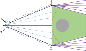
This paper will focus on the sphere, being the experimental test model, which is commonly used for important fundamental studies, with its centre positioned on the nozzle centreline. The divergent free stream from a conical nozzle can be modelled as a steady spherical source flow (Inouye Reference Inouye1966; Lin et al. Reference Lin, Reeves and Siegelman1977; Golovachov Reference Golovachov1985; Hornung Reference Hornung2019; Farokhi Reference Farokhi2021), as shown in figure 2. One can define  $d = L_{1}/R_{s}$, which measures the degree of non-uniformity, where $R_{s}$ is the radius of the sphere and $L_{1}$ is the distance between the centre of the source and the shock wave on the axisymmetry axis; $d = \infty$ then corresponds to a uniform flow. The sphere is usually positioned near the nozzle exit such that the centre of the shock front lies on the nozzle exit plane, as shown in figure 2. In this case, the nozzle half-angle $\phi$ can be related to $d$ via $\tan (\phi ) = k/d$, where $k$ is a measure of how big the spherical test model is relative to the nozzle exit; $k = 2$ would correspond to a large test model with a flow field which roughly takes up all the core flow space while $k = 10$ would correspond to a small Pitot or heat flux probe. The half-angle of the conical nozzles used on hypersonic impulse facilities, past and present, varies between $5.8^{\circ }$ and $15^{\circ }$, as shown in figure 1. Depending on the relative size of the test model ( $k$), the degree of non-uniformity can realistically be around $d = 4\unicode{x2013}100$ in the experiments. More precisely, the value of $d$ in practice will be slightly higher than this due to the boundary layer in the nozzle which generally reduces the effective nozzle half-angle from the geometric one reported in figure 1. Also, as mentioned earlier, the test model is normally placed near the nozzle exit, where the core flow is largest (since wind tunnel nozzles are always underexpanded, the core flow gets smaller downstream due to the expansion fan originating from the wall corner at the nozzle exit, as shown in figure 2). If, for whatever reason, the model is placed some distance downstream of the nozzle exit, the effect would be to increase ‘ $d$’ (because $L_{1}$ is increased) and reduce the influence of free-stream conicity. Additionally, if one really wanted to do this, it would probably be necessary to use a smaller model as well due to the reduced core flow, which will further increase ‘ $d$’ (because $R_{s}$ is decreased). Consequently, the lower bound of $d = 4$ stated above can duly be considered a conservative estimate of the maximum influence of free-stream conicity that may be encountered in practice.

Figure 2. The schematic of the diverging free stream upstream of a spherical test model generated by a conical nozzle, which always operates in underexpanded mode in wind tunnels.
In this paper, we will examine how much effect this non-uniformity can have on the various aspects of the flow over the spherical test model on the forebody – such as the shock wave, pressure, heat flux, boundary layer and tangential velocity gradient – under different flow conditions and gas states. Both analytical and numerical methods will be used, and the results between the two will be compared. The numerical work will include thermochemical non-equilibrium simulations; this is unlike the previous studies that examine the influence of free-stream conicity, which only consider perfect-gas or equilibrium flows (Inouye Reference Inouye1966; Lunev & Khramov Reference Lunev and Khramov1970; Shapiro Reference Shapiro1975; Lin et al. Reference Lin, Reeves and Siegelman1977; Eremeitsev & Pilyugin Reference Eremeitsev and Pilyugin1981, Reference Eremeitsev and Pilyugin1984; Golovachov Reference Golovachov1985; Hornung Reference Hornung2019). Also unlike the previous works, the results here will be fully related to practical experimental scenarios by considering the realistic range of ‘ $d$’ and by considering the uncertainties (measurement uncertainties and shot-to-shot variations) of hypersonic experiments. In addition to answering the aforementioned important question of just how much the free-stream conicity influences the experiments, the underlying physics involved will be thoroughly explained as well, which is not discussed in many of the earlier works which mostly only look to predict and quantify the influence of free-stream conicity without really attempting to provide a physical explanation for the observations.
2. Methodology
2.1. Analytical method
An appreciable amount of theoretical work exists in the literature (mostly done by Russian researchers during the 1970s and 1980s) to describe the influence of hypersonic free-stream conicity on the flow over a sphere. In these studies, analytical equations have been derived which predict how much effect a divergent free stream has on the various aspects of the flow over a spherical test model. More precisely, these works compare conical free streams with the equivalent uniform free streams, where the free-stream properties immediately ahead of the shock on the symmetry axis are identical. From these past studies, a comprehensive analytical model is subsequently compiled for use in the current work, which is described as follows, aided by figures 3 and 4.

Figure 3. Flow field around a sphere in a conical free stream with the nomenclatures.

Figure 4. Flowchart describing the operation of the analytical model. The blue boxes are the parameters to be predicted, the yellow boxes are the predictors and the green boxes are the inputs (other than trivial free-stream values) to the predictors.
To quantify the influence of the free-stream conicity on the shock stand-off distance on the symmetry axis, Shapiro (Reference Shapiro1975) gave
 \begin{equation} \frac{\varDelta^{0}}{\varDelta^{0}_\infty} = \frac{\theta^{s}}{\theta^{s}_\infty} \frac{1}{1+\varDelta^{0}_\infty\left(1-\dfrac{\theta^{s}}{\theta^{s}_\infty}\right)}, \end{equation}
where  $\varDelta ^{0}$ and $\varDelta ^{0}_\infty$ are the shock stand-off distances on the symmetry axis for a non-uniform and uniform free stream, respectively, and
 \begin{equation} \frac{\theta^{s}}{\theta^{s}_\infty} = \frac{1}{2} \left[\left(\frac{1+\varDelta^{0}_\infty}{\varDelta^{0}_\infty}+1\right) - \sqrt{\left(\frac{1+\varDelta^{0}_\infty}{\varDelta^{0}_\infty}-1\right)^2+\frac{4}{l}\frac{1+\varDelta^{0}_\infty}{\varDelta^{0}_\infty}}\right], \end{equation}
where  $\theta ^{s}$ and $\theta _{\infty }^{s}$ are the locations (angle from the symmetry axis) of the sonic point on the boundary layer edge (or surface of the sphere for inviscid flows) for a non-uniform and uniform free stream, respectively, and $l$ is the distance between the centre of the source and centre of the sphere. The above equations were derived, without needing to define any gas properties, based on geometric considerations of the shock wave, sphere and conical free stream, and assuming the normalized distribution of the shock stand-off distance, $\varDelta /\varDelta ^{0}$, is independent of the degree of free-stream conicity when given as a function of $\eta = \theta /\theta ^{s}$ instead of $\theta$ (that is, $\theta$ is normalized with that of the sonic point). The above equations, along with the assumption of $\varDelta /\varDelta ^{0}$ being a universal function of $\eta$, are shown by Shapiro (Reference Shapiro1975) and Golovachov (Reference Golovachov1985) to work well after comparing with both viscous and inviscid computational fluid dynamics (CFD) simulations for a range of Mach numbers (3–10), Reynolds numbers (177–35 500) and $d$ (0.3–25) for both perfect-gas and equilibrium flows. The above equations require $\varDelta ^{0}_\infty$ a priori, which can be calculated analytically with (Lobb Reference Lobb1964)
 \begin{equation} \varDelta^{0}_\infty = 0.82R_{s}\frac{\rho_{1}}{\rho_{2}}, \end{equation}
where  $\rho _{1}$ and $\rho _{2}$ are the flow densities before and after the shock on the symmetry axis, respectively. This correlation is obtained based on the numerical results of Van Dyke (Reference Van Dyke1958) for a perfect gas for Mach numbers between 1.5 and 10.
Recently, Hornung (Reference Hornung2019) independently derived another expression describing the influence of the free-stream conicity on the shock stand-off distance on the symmetry axis based on a control volume conservation of mass argument with geometric relations, without needing to specify any gas properties, while assuming the shock-parallel component of velocity is constant across the shock layer. Further assuming the average density across the shock layer remains constant with varying free-stream conicity, which is true for perfect-gas or equilibrium flows, one can derive
 \begin{equation} \frac{\varDelta^{0}}{\varDelta^{0}_\infty} = \frac{1}{1+\dfrac{\left(R_{c}^{0}\right)_{\infty}}{L_{1}}}, \end{equation}
where  $(R_{c}^{0})_{\infty }$ is the radius of curvature of the shock on the symmetry axis in a uniform free stream, which can be calculated analytically with the semi-empirical correlation of Billig (Reference Billig1967) for a perfect gas with $\gamma = 1.4$
 \begin{equation} \left(R_{c}^{0}\right)_{\infty} = 1.143\exp\left(\frac{0.54}{\left(M-1\right)^{1.2}}\right)R_{s}, \end{equation}
where  $M$ is the free-stream Mach number.
To describe the influence of the free-stream conicity on the stagnation point heat flux, Eremeitsev & Pilyugin (Reference Eremeitsev and Pilyugin1981) gave
 \begin{equation} \frac{q^{0}}{q^{0}_\infty} = \sqrt{1+\frac{R_{s}}{L_{2}}}, \end{equation}
where  $L_{2}$ is the distance between the centre of the source and the stagnation point on the sphere ( $L_{2} = L_{1} + \varDelta ^{0}$). This equation is derived, without considering finite-rate thermochemistry, based on the self-similar boundary layer theory of Lees (Reference Lees1956) with the boundary layer edge conditions obtained using thin shock-layer theory, where $M_{\infty } \rightarrow \infty$ and $\gamma _{\infty } \rightarrow 1$. In such a limit, the wall-normal gradient of the flow properties is assumed to be large compared with their tangential gradient, and the shock shape, the body shape and the streamline shapes are assumed to be all the same. Analytical expressions for the boundary layer edge properties are obtained, according to the method of Chernyi (Reference Chernyi1961), by replacing the flow variables in the von Mises formulation of the governing equations by their power series expansion truncated after the first term, which is then used with Lees’ theory to obtain (2.6). As suggested by this equation, the gas model-dependent terms disappear, indicating $q^{0}/q^{0}_\infty$ can be predicted without specifying any gas properties.
An alternative expression for  $q^{0}/q^{0}_\infty$ can be derived as follows. Because the free-stream conicity does not change the flow properties at the stagnation point – such as the pressure, density, temperature and enthalpy – for a perfect or equilibrium gas (Shapiro Reference Shapiro1975; Golovachov Reference Golovachov1985), the change in the stagnation point heat flux, in this case, comes purely from the change in the tangential velocity gradient at the boundary layer edge on the stagnation streamline, $({\rm d}u/{{\rm d}\kern0.06em x})^{0,e}$, according to Fay & Riddell (Reference Fay and Riddell1958) with
 \begin{align} q^{0} \propto \sqrt{\left(\frac{{\rm d}u}{{\rm d}\kern0.06em x}\right)^{0,e}}, \end{align}
assuming a perfect or equilibrium gas. Following from Olivier (Reference Olivier1995), who obtained an analytical expression for the tangential velocity gradient after an integral method is used to solve the two-dimensional conservation equations for the stagnation point without needing to specify any gas properties, the tangential velocity gradient assuming a perfect or equilibrium gas can be derived as
 \begin{equation} \left(\frac{{\rm d}u}{{\rm d}\kern0.06em x}\right)^{0,e} \propto \frac{R_{s}+\varDelta^{0}}{\varDelta^{0}}. \end{equation}
Therefore, one can write
 \begin{equation} \frac{q^{0}}{q^{0}_\infty} = \sqrt{\frac{R_{s}+\varDelta^{0}}{\dfrac{\varDelta^0}{\varDelta^0_{\infty}}R_{s}+\varDelta^{0}}}. \end{equation}
Alternatively, Shapiro (Reference Shapiro1975) proposed another expression for predicting the influence of free-stream conicity on the tangential velocity gradient given as
 \begin{equation} \frac{\left(\dfrac{{\rm d}u}{{\rm d}\kern0.06em x}\right)^{0,e}}{\left(\dfrac{{\rm d}u}{{\rm d}\kern0.06em x}\right)^{0,e}_\infty} = \frac{\theta^{s}_\infty}{\theta^{s}}, \end{equation}
which is simply derived assuming the tangential velocity gradient remains constant along the boundary layer edge between the axisymmetry axis and the sonic point. Combining (2.7) and (2.10) gives
 \begin{equation} \frac{q^{0}}{q^{0}_\infty} = \sqrt{\frac{\theta^{s}_\infty}{\theta^{s}}}. \end{equation}
Analytical methods also exist to describe the influence of the free-stream conicity on the flow property distributions in the flow around the sphere. For the normalized surface heat flux distribution, Eremeitsev & Pilyugin (Reference Eremeitsev and Pilyugin1984) gave, based on a similar method to what they used in their previous work (Eremeitsev & Pilyugin Reference Eremeitsev and Pilyugin1981) discussed above involving thin shock-layer and self-similar boundary layer theories,
 \begin{equation} \frac{\dfrac{q}{q^{0}}}{\left(\dfrac{q}{q^{0}}\right)_{\infty}} = \left[\cos\left(\theta\right)\right]^{({R_{s}}/{3L_{2}})({5R_{s}}/{L_{2}}+8)}, \end{equation}
where  $\theta$ is the angle from the symmetry axis of some point on the sphere's surface, and $q/q^{0}$ is the normalized heat flux (normalized by the value at the stagnation point). Subscript $\infty$ indicates the uniform free-stream result as usual. Again, finite-rate thermochemistry is not considered in the derivation, and the gas property-dependent terms disappear.
For the normalized surface pressure distribution, Lunev & Khramov (Reference Lunev and Khramov1970) gave, based on the classic Newtonian theory for spheres and accounting for the conically expanding free stream,
 \begin{equation} \frac{\dfrac{p_{s}}{p_{s}^{0}}}{\left(\dfrac{p_{s}}{p_{s}^{0}}\right)_{\infty}} = \frac{\left(\rho u^{2}\right)_{\theta}}{\left(\rho u^{2}\right)_{\theta=0}} \frac{\cos^{2}(\omega+\theta)}{\cos^{2}(\theta)}, \end{equation}
where  $\omega$ is the flow divergence angle at $\theta$, $p_{s}/p_{s}^{0}$ is the normalized surface pressure (normalized by the Pitot pressure) and $(\rho u^{2})_{\theta }$ is the local ram pressure on the sphere surface, assuming an ideal Newtonian flow, at $\theta$. The value of $(\rho u^{2})_{\theta }$ at different locations can be calculated from the governing equations for a steady spherical source flow in closed form which, for a perfect gas, is (Golovachov Reference Golovachov1985)
 \begin{equation} \left. \begin{gathered} U=\left(\frac{r^\ast}{r}\right)^2\left(\frac{2}{\gamma+1}\right)^{{1}/({\gamma-1})} \left(1-\frac{\gamma-1}{\gamma+1}U^2\right)^{-({1}/({\gamma-1}))},\\ \frac{p}{p^\ast}=\left(\frac{r^\ast}{r}\right)^2\left(1-\frac{\gamma-1}{\gamma+1}U^2\right)\left(\frac{\gamma+1}{2U}\right),\\ \frac{\rho}{\rho^\ast}=\left(\frac{r^\ast}{r}\right)^2\left(\frac{1}{U}\right), \end{gathered} \right\} \end{equation}
where  $\gamma$, $p$,
$p$,  $\rho$ and $U = u/u^{*}$ are the heat capacity ratio, static pressure, density and normalized value of the velocity $u$ in the source flow at a distance of $r$ from the source centre. The superscript ‘ $*$’ values represent the properties at $r^{*}$, where $u=u^\ast =\sqrt {\gamma p^\ast /\rho ^\ast }$ ( $M = 1$). Newtonian theory is essentially a pure fluid mechanics theory and does not consider the thermodynamics, which makes it suitable for pressure predictions since the pressure behind a strong shock wave is only weakly dependent on the thermodynamics (Chernyi Reference Chernyi1961; Anderson Reference Anderson2019).
Furthermore, Shapiro (Reference Shapiro1975) proposed a transformation, where the distribution is given in terms of  $\eta = \theta /\theta ^{s}$ instead of $\theta$, allowing all the results (non-uniform and uniform) to coalesce, as mentioned earlier in this section. In other words, the distributions become independent of the degree of free-stream conicity when the distributions are considered functions of $\eta$. This transformation, discovered via analysis of numerous numerical simulations, is suggested to work not only on the shock stand-off distance distribution, but also on the surface pressure and heat flux distributions regardless of the gas type for both frozen and equilibrium flows (Shapiro Reference Shapiro1975; Golovachov Reference Golovachov1985). With this transformation, one can obtain the distributions in some non-uniform free streams given that the corresponding distribution in the equivalent uniform free stream and the sonic point ratio $\theta ^{s}/\theta ^{s}_\infty$ are known. For a uniform free stream, the normalized pressure distribution can be obtained analytically from Newtonian flow theory (Anderson Reference Anderson2019)
 \begin{equation} \left(\frac{p_s}{p_s^0}\right)_\infty=\cos^2{\left(\theta\right)}, \end{equation}
which works for any hypersonic flow. The normalized heat flux distribution can be obtained analytically from (Murzinov Reference Murzinov1966)
 \begin{equation} \left(\frac{q}{q^0}\right)_\infty=0.55+0.45cos{\left(2\theta\right)}, \end{equation}
which is correlated from numerous equilibrium simulations, but is shown to also work well for both non-reacting (Wang, Bao & Tong Reference Wang, Bao and Tong2010; Gu et al. Reference Gu, Olivier, Wen, Hao and Wang2022) and non-equilibrium (Voronkin & Geraskina Reference Voronkin and Geraskina1969) simulations. The normalized shock stand-off distance distribution can be obtained analytically from the semi-empirical correlation of Billig (Reference Billig1967)
 \begin{align} \left. \begin{gathered} \left(\frac{\varDelta}{\varDelta^{0}}\right)_{\infty}=\frac{\sqrt{z^{2}+y^{2}}-R_{s}}{\varDelta^{0}_{\infty}},\\ \theta=\tan^{{-}1}{\left(\frac{y}{z}\right)},\\ z=R_{s}+\varDelta^{0}_\infty-\left(R_{c}^0\right)_{\infty}\cot^{2}\left(\sin^{{-}1}\left(\frac{1}{M}\right)\right)\left[\sqrt{1+\frac{y^2\tan^2\left(\sin^{{-}1}\left(\dfrac{1}{M}\right)\right)}{\left(R^{0}_{c}\right)^{2}_{\infty}}}-1\right], \end{gathered} \right\} \end{align}
who assumed the shock shape is a hyperbola that asymptotes to the free-stream Mach angle, which is a good approximation for the shock over a sphere in any hypersonic flow (Hornung Reference Hornung2010; Zander et al. Reference Zander, Gollan, Jacobs and Morgan2014).
For predicting the influence of free-stream conicity on the normalized shock stand-off distance distribution, an alternative transformation may be proposed in which all the results (non-uniform and uniform) are assumed to coalesce when the distribution is given in terms of  $\theta +\omega$ (where $\omega$ is the flow divergence angle at $\theta$, defined earlier in this section) instead of $\theta$. That is, it assumes that the normalized shock stand-off distance at some $\theta = \theta _{1}$ in a uniform flow is equal to that at $\theta = \theta _{1}-\omega$ in a non-uniform flow.
Overall, the analytical model is summarized in figure 4, which can be used to accurately predict (shown later in this paper) the influence of free-stream conicity on various aspects of the flow over a sphere. This analytical model is formed by different analytical equations which are used together to make the predictions without needing any input from CFD. Although, many of these equations in our analytical model are derived by others (except (2.9) and (2.11), and the transformation of the normalized shock stand-off distance distribution, which are our own contributions), using these analytical equations together in the way described in figure 4 is an important original contribution of the current work. For example, Shapiro's transformation requires the corresponding distribution in a uniform free stream as an input, which was originally obtained from CFD (Shapiro Reference Shapiro1975; Golovachev & Leont'eva Reference Golovachev and Leont'eva1983; Golovachov Reference Golovachov1985) but we propose the use of analytical expressions for this in our model, allowing for a more practical, fully analytical way of determining the influence of free-stream conicity. Similar can be said for many of the other equations in our analytical model. Therefore, aside from bringing together relevant equations that have been scattered throughout the literature and providing original commentaries regarding the derivation and limitations of these analytical expressions, a methodology is given for using these equations together to accurately predict the influence of free-stream conicity without needing any input from CFD. Furthermore, the compilation and subsequent visual description of the model shown in figure 4 allows us to also gain insight into the relationship among how the different parameters are influenced by the free-stream conicity. From this, it can be seen that  ${\theta ^{s}}/{\theta ^{s}_\infty }$ is the most fundamental parameter characterizing the influence of the free-stream conicity which can be related to every other parameter.
Most of the predictors for the influence of free-stream conicity (yellow boxes in figure 4) used as part of our analytical model have never been compared with CFD before (e.g. (2.1), (2.8), (2.10), (2.9), (2.11), (2.12) and (2.13)). Even for the equations that have been compared with CFD before, most of them have not been compared with modern-day CFD results (e.g. (2.2), (2.6) and Shapiro's transformation); the older CFD simulations they were compared with are less accurate as they either first solved the Euler equations to get the inviscid flow field, which is then used as the boundary layer edge condition to solve the boundary layer equations (Golovachov Reference Golovachov1985), or used very few grids (e.g.  $7 \times 26$ in the tangential and wall-normal directions, respectively) when solving the Navier–Stokes equations (Golovachev & Leont'eva Reference Golovachev and Leont'eva1983). Therefore, it is not immediately clear whether our analytical model could give accurate enough results, and a systematic validation is, thus, required to find out. As will be presented later in this paper, good agreement is observed between our analytical model and CFD for a range of flow conditions (different Mach and Reynolds numbers, and gas models), which is a non-trivial and important result. Furthermore, the results of this comparison when considered together with how the analytical equations were derived allow further insights to be revealed regarding the physical problem.
None of the equations given above in this section explicitly consider thermochemical non-equilibrium effects in their derivation (which is expected considering there are rarely analytical solutions when finite-rate thermochemistry is involved). However, this is not an issue because, as will be shown later on in this paper, the influence of the free-stream conicity is mostly insensitive to non-equilibrium effects. This may be expected considering Shapiro (Reference Shapiro1975) and Golovachov (Reference Golovachov1985) have shown that the influence of free-stream conicity is mostly independent of the flow condition, type of gas and whether the gas is in equilibrium or frozen; the same can be deduced from the derivations of Hornung (Reference Hornung2019), Lunev & Khramov (Reference Lunev and Khramov1970) and Eremeitsev & Pilyugin (Reference Eremeitsev and Pilyugin1981, Reference Eremeitsev and Pilyugin1984), who demonstrated that it may be unnecessary to specify the thermodynamic properties of the gas when predicting the influence of free-stream conicity, as mentioned above. Thus, it is found that good predictions of the influence of free-stream conicity are made by the current analytical model even when the flow is in thermochemical non-equilibrium.
2.2. Numerical method
The Navier–Stokes solver ‘Eilmer’ from The University of Queensland is used for the current work. As shown by Gollan & Jacobs (Reference Gollan and Jacobs2013) and Gibbons et al. (Reference Gibbons, Damm, Jacobs and Gollan2023), Eilmer is a validated and established tool for the simulation of various hypersonic flows, including frozen (perfect gas), thermochemical equilibrium and thermochemical non-equilibrium flows. Accurate predictions of the flow field and wall heat flux in such conditions are demonstrated by comparing them with experimental measurements (Deepak, Gai & Neely Reference Deepak, Gai and Neely2012; Jacobs et al. Reference Jacobs, Gollan, Jahn and Potter2015; Park, Gai & Neely Reference Park, Gai and Neely2016). Due to the reliability of the code, it has been used as a validation tool for new models of high-enthalpy blunt-body viscous flows (Yang & Park Reference Yang and Park2019; Ewenz Rocher et al. Reference Ewenz Rocher, Hermann, McGilvray and Gollan2021; Gu et al. Reference Gu, Olivier, Wen, Hao and Wang2022).
Eilmer is an open-source explicit Navier–Stokes solver for transient compressible flow in two and three dimensions based on the integral form of the Navier–Stokes equations. The core gas dynamics formulation is based on finite-volume cells. The inviscid fluxes are calculated at the cell interfaces using an adaptive flux calculator in which the Harten–Lax–van Leer–Einfeldt scheme (Einfeldt Reference Einfeldt1988) is applied near shocks and the Roe scheme (Roe Reference Roe1981) is applied elsewhere; as discussed by Nishikawa & Kitamura (Reference Nishikawa and Kitamura2008), this resolves the problem of simulating flow fields containing flow features that require low dissipation schemes to accurately capture but also containing discontinuities which require high dissipation schemes to avoid numerical instabilities (e.g. the carbuncle problem). The viscous fluxes are calculated using the averaged values of the viscous stresses at the cell vertices. A modified van Albada limiter (van Albada, van Leer & Roberts Reference van Albada, van Leer and Roberts1997) and a monotonic upstream-centred scheme for the conservation laws’ (van Leer Reference van Leer1979) reconstruction scheme are used to obtain second-order spatial accuracy. The time advancement procedure is based on the operator-splitting method (Oran & Boris Reference Oran and Boris2001) and the time integration uses the implicit first-order Runge–Kutta method (Petzold Reference Petzold1986). Numerical stability is maintained by the Courant–Friedrichs–Lewy (CFL) criterion, with a CFL value of 0.5 used in the current work. For thermochemical non-equilibrium simulations, Park's two-temperature model (Park Reference Park1993) is used, in which the dissociation/recombination reactions are controlled by an effective temperature,  $T_{c}$, given as $T_{c}=T_{tr}^{0.5}T_{v}^{0.5}$, where $T_{tr}$ is the translational–rotational temperature and $T_{v}$ is the vibrational temperature. The thermochemical effects are handled with specialized updating schemes that are coupled into the overall time-stepping scheme. The species mass diffusion is modelled using Fick's first law assuming binary diffusion (Anderson Reference Anderson2019). The heat flux for thermochemical non-equilibrium flows is calculated via the formulation given by Gupta et al. (Reference Gupta, Yos, Thompson and Lee1990). The reader is referred to Gollan & Jacobs (Reference Gollan and Jacobs2013), Gibbons et al. (Reference Gibbons, Damm, Jacobs and Gollan2023) and Jacobs et al. (Reference Jacobs, Gollan, Denman, O'Flaherty, Potter, Petrie-Repar and Johnston2010) for further details on Eilmer, including its formulation and validation. The current work makes use of the existing features of the code without any further development.
The numerical test conditions are shown in table 1. Conditions 1–4 originate from a reservoir pressure and temperature of 2 MPa and 800 K, respectively, which are representative of conditions in a cold hypersonic (low-enthalpy) facility (Schrijer & Bannink Reference Schrijer and Bannink2010). Condition 3 is the same as condition 2 except the sphere is larger. Condition 5 is a high-enthalpy condition corresponding to the HEG condition H12R0.39 (Hannemann et al. Reference Hannemann, Martinez Schramm, Wagner and Ponchio Camillo2018; Shen et al. Reference Shen, Shao, Ji, Chen, Lu and Ma2023). Condition 6 is the same as condition 5 except thermochemical equilibrium is assumed. The free-stream chemical composition (mass fraction) in the perfect-gas and equilibrium simulations is  $N_{2} = 0.767$ and $O_{2} = 0.233$, while that in condition 5 (the non-equilibrium simulation) is $N_{2} = 0.7417$, $\textrm {N} = 0.0$, $O_{2} = 0.1634$, $O=0.0454$ and $\textrm {NO} = 0.0495$. Condition 5 has a free-stream vibrational temperature of 2300 K. Although variants of air are explicitly used as the test gas here, the results presented later in this paper are not limited to this gas because the influence of free-stream conicity is mostly insensitive to the flow condition and type of gas, as have been shown (Lunev & Khramov Reference Lunev and Khramov1970; Shapiro Reference Shapiro1975; Eremeitsev & Pilyugin Reference Eremeitsev and Pilyugin1981, Reference Eremeitsev and Pilyugin1984; Golovachov Reference Golovachov1985; Hornung Reference Hornung2019) for some properties in the flow over a sphere and will be further demonstrated later in this paper for some more properties, considering PG air and EQ air are essentially different types of gas with totally different species composition.
Table 1. The numerical test conditions. Here, ‘PG’, ‘EQ’ and ‘NONEQ’ refer to perfect gas, thermochemical equilibrium and thermochemical non-equilibrium simulations, respectively,  $p_{\infty }$, $T_{\infty }$, $u_{\infty }$ and $M_{\infty }$ are the free-stream static pressure, temperature, velocity and Mach number. The Reynolds number, $Re$, is calculated using the free-stream properties and $R_{s}$.

The computational domain and the boundary conditions used for the current work are shown in figure 5. The simulation is two-dimensional and axisymmetric, which is enough for the intents and purposes of the current work (three-dimensional simulations of such flows are known to be very difficult and contain significant numerical error, as discussed by Candler et al. (Reference Candler, Barnhardt, Drayna, Nompelis, Peterson and Subbareddy2007); therefore, there is really not much to be gained and a lot to be lost if one chooses to compute in three dimensions for the current work).

Figure 5. The computational domain, boundary conditions and mesh. The wall temperature  $T^{w}$ is fixed at 295 K.
For condition 5, both a non-catalytic (NC, where no catalytic interaction occurs between gas and surface) and super-catalytic (SC, where instantaneous equilibration of the gas occurs at the surface) wall are tested, which correspond to surface reaction Damköhler numbers of 0 and  $\infty$, respectively (Inger Reference Inger1963). Relating to real applicability, an NC wall would correspond to some glass surfaces while an SC wall would correspond to some metallic surfaces (Goulard Reference Goulard1958). The surface catalycity is really only relevant for thermochemical non-equilibrium simulations. For perfect-gas simulations, the chemical composition in the fluid remains a perfect air mixture (mass fractions of $N_{2} = 0.767$ and $O_{2} = 0.233$); therefore, nothing can happen at the wall due to surface catalycity since the chemical composition of the fluid at the wall is already in equilibrium at the corresponding wall temperature (295 K). Likewise, for equilibrium simulations, the local chemical composition of the fluid is always in equilibrium at the local temperature; therefore, the fluid at the wall is also in equilibrium at the corresponding wall temperature, which means that surface catalycity cannot have any influence here. Consequently, surface catalycity can only impact non-equilibrium simulations (e.g. condition 5 in the current work).
The inflow boundary is made to be adaptive and fit with the shock front. The free-stream conditions shown in table 1 correspond to those of the uniform free stream, which in turn correspond to the free-stream conditions immediately ahead of the shock on the symmetry axis in the case of a non-uniform free stream ( $r = L_1$ in figure 5) which is modelled as a spherical source flow. Subsequently, for the non-uniform free-stream simulations, the flow state on the inflow faces has to be computed from the governing equations of a steady spherical source flow in differential form in spherical coordinates given as (Crittenden & Balachandar Reference Crittenden and Balachandar2018)
 \begin{equation} \left. \begin{gathered} \partial\left(r^2\rho u_r\right)=0,\\ \partial p+{\rho u}_r\partial u_r=0,\\ \partial h+u_r\partial u_r=0, \end{gathered} \right\} \end{equation}
where  $h$ is the specific enthalpy and $u_{r}$ is the radial velocity. The solution is numerically obtained with the equation of state after specifying the location of the source centre and the flow condition at some specific distance of $r$ from the source centre. Different locations for the source centre are tested such that $d$ = 4, 25 and 100 are examined for each condition in table 1. We specify the flow condition at $r = L_1$, which is given in table 1, and the flow state on the inflow faces is computed according to (2.18), as mentioned above. A frozen source flow is assumed for conditions 1–5 while an equilibrium source flow is assumed for condition 6.
A structured grid of  $240 \times 240$ is used, which is similar to that used in other comparable works from the recent literature (Fahy et al. Reference Fahy, Buttsworth, Gollan, Jacobs, Morgan and James2021; Luo et al. Reference Luo, Wang, Li, Zhao and Gu2023; Guo, Wang & Li Reference Guo, Wang and Li2024). Strong clustering is implemented at the shock front and normal to the wall, as shown in figure 5. The clustering at the shock front is regular, with a spacing of around $0.5\unicode{x2013} 2.0\, \mathrm {\mu }\textrm {m}$ while the clustering normal to the wall decreases in the radial direction with a minimum cell spacing of around $0.05\unicode{x2013} 1.0\,\mathrm {\mu }\textrm {m}$ at the first cell from the wall at the stagnation point, depending on the condition. Mild clustering is made in the wall-tangential direction towards the axisymmetry axis, as shown in figure 5. The minimum spacing in the tangential direction, which is found on the first cell from the axisymmetry axis, is around $10\,\mathrm {\mu }\textrm {m}$. The average spacing in the wall-normal and wall-tangential directions is around $15\,\mathrm {\mu }\textrm {m}$ and $85\,\mathrm {\mu }\textrm {m}$, respectively.
For predicting the surface heat flux, various computational scientists have stated that the wall cell Reynolds number,  $Re_{wall}$, needs to be below a certain value. Some authors state that any $Re_{wall}$ value below 3 would give good results (Papadopoulos et al. Reference Papadopoulos, Venkatapathy, Prabhu, Loomis and Olynick1999), while other authors state that the $Re_{wall}$ value should be around 1 (Ren et al. Reference Ren, Yuan, He, Zhang and Cai2019). The latter condition is achieved for the current work using a $240 \times 240$ grid for all the simulated cases, as shown exemplarily in figure 6(a) for condition 5. A mesh independence study is carried out for each test case by testing with scaled meshes and comparing the heat flux distribution around the sphere, which is influenced by many aspects of the flow field and is the most grid-sensitive parameter (Candler et al. Reference Candler, Barnhardt, Drayna, Nompelis, Peterson and Subbareddy2007; Mazaheri & Kleb Reference Mazaheri and Kleb2007; Kitamura et al. Reference Kitamura, Shima, Nakamura and Roe2010; Gu et al. Reference Gu, Olivier, Wen, Hao and Wang2022). An example is shown in figure 6(b) for condition 5; the result is essentially converged when more than $120 \times 120$ cells are used, and similarly for the other test cases. Therefore, all the numerical results presented in the subsequent sections, which are obtained using a $240 \times 240$ grid, are converged. An estimated representative uncertainty of less than ${\pm }0.5\ \%$ can be given to the computed stagnation point heat flux (Gu et al. Reference Gu, Olivier, Wen, Hao and Wang2022), which is already the most uncertain property calculated in these kinds of simulations (Capriati et al. Reference Capriati, Cortesi, Magin and Congedo2022). Hence, the numerical uncertainties of the current simulations can be considered negligible for the intent and purposes of the current work. Further validation of these numerical results is implied from the excellent agreement with the analytical/theoretical results, as will be shown below in § 4.

Figure 6. The wall (a) cell Reynolds number and (b) heat flux for condition 5 (NONEQ) with a non-uniform free stream of  $d = 4$ and a non-catalytic wall. The angle is in degrees.
3. Experimental uncertainties
Before presenting the results examining the influence of free-stream conicity on the flow over a sphere, it is necessary to first define the representative experimental uncertainties for the flow properties of interest. This work is essential because the importance of free-stream conicity must later be interpreted in relation to the experimental uncertainties (e.g. if the influence of free-stream conicity is small relative to the experimental uncertainties, then one may suggest that free-stream conicity is unimportant, and vice versa). The uncertainties are summarized in table 2. The total uncertainty is considered the sum of the measurement uncertainty, which is the uncertainty originating from the measurement-taking device/method, and the test condition repeatability, which is the uncertainty originating from the facility generating a slightly different test condition in each shot.
Table 2. Representative experimental uncertainties.

For the shock stand-off distance,  $\varDelta$, measured via imaging, the measurement uncertainty reported in the literature ranges from approximately $5\,\%$– $10\,\%$ (Zander et al. Reference Zander, Gollan, Jacobs and Morgan2014; Sudhiesh Kumar & Reddy Reference Sudhiesh Kumar and Reddy2016). Assuming that the total uncertainty is manifested as the shot-to-shot variation of repeated measurements of $\varDelta$ at a given nominal test condition, this is reported to be around $15\,\%$ (Zander et al. Reference Zander, Gollan, Jacobs and Morgan2014). Consequently, the contribution to the total uncertainty from the test condition repeatability is around 5 %–10 %. For the surface heat flux, the measurement uncertainty of measurements made using coaxial thermocouples is reported to be around 5 %–10 % (Park et al. Reference Park, Neeb, Plyushchev, Leyland and Gülhan2021). The shot-to-shot variation of coaxial thermocouple heat flux measurements made at various locations on the surface of a 39 mm diameter sphere in the TH2 reflected shock tunnel at two different test conditions (Gu et al. Reference Gu, Olivier, Wen, Hao and Wang2022) is presented in figure 7(a). Also included in the figure, and treated as shot-to-shot variations, are measurements made in the same shot at the same angle from the stagnation point but at opposite locations on the sphere (mirror measurements). Independent of the angle from the stagnation point, the results indicate a total uncertainty of around 20 %–30 %, which is also consistent with the data in Rose & Stark (Reference Rose and Stark1958) and Eitelberg, Krek & Beck (Reference Eitelberg, Krek and Beck1996), with the test condition repeatability contributing approximately 15 %–20 %.

Figure 7. The relative shot-to-shot and mirror measurement variation of (a) the absolute heat flux measurements, and (b) the normalized heat flux measurements, on a 39 mm diameter sphere. The upper-bar symbol denotes the average value. The angle is in degrees.
The normalized heat flux,  $q/q^{0}$, and surface pressure, $p/p^{0}$, distributions are known to be rather insensitive to the free-stream condition (and the type of gas) (Lees Reference Lees1956; Murzinov Reference Murzinov1966; Anderson Reference Anderson2019). The same is found for the normalized shock stand-off distance distribution, $\varDelta /\varDelta ^{0}$, as shown in figure 8, obtained using (2.17); although this equation still contains the Mach number, shock stand-off distance and shock radius of curvature, which are free-stream-dependent quantities (unlike the equations for $q/q^{0}$ and $p/p^{0}$ which contain no such quantities), their influence on the result is rather weak. Therefore, the test condition repeatability will not contribute to the total uncertainty for these normalized distribution measurements. The total uncertainty would then be just the measurement uncertainty which, for these normalized measurements, would be two times the measurement uncertainty of the absolute measurements since these normalized measurements are obtained as a quotient of two absolute measurements. This results in total uncertainties of around $\pm$10 %–20 % for the normalized shock stand-off distance and heat flux measurements, and $\pm$6 %–12 % for the normalized surface pressure measurements.

Figure 8. The normalized shock stand-off distance distribution obtained using (2.17). The angle is in degrees.
For the normalized surface pressure and heat flux uncertainties estimated here, experimental data are available for comparison. Shot-to-shot and mirror measurement scatters of the normalized surface pressure are reported by Karl, Martinez Schramm & Hannemann (Reference Karl, Martinez Schramm and Hannemann2003) and Rose & Stark (Reference Rose and Stark1958); variations of around  $\pm$5 %–10 % are observed, which is consistent with the estimated uncertainty in table 2. Shot-to-shot and mirror measurement scatters of the normalized heat flux taken in TH2 are shown in figure 7(b); independent of the angle from the stagnation point, variations of around $\pm$10 %–20 % are observed, which is exactly consistent with the estimated value in table 2. The experimental data reported by Karl et al. (Reference Karl, Martinez Schramm and Hannemann2003) and Eitelberg et al. (Reference Eitelberg, Krek and Beck1996) show further consistency. Also, the scatter of the normalized values in figure 7(b) is distinctly smaller than that of the absolute values in figure 7(a), providing further confirmation of the role of the test condition repeatability discussed earlier. As shown in table 2, the test condition repeatability contributes significantly to the total uncertainty of $\varDelta$ and $q$ measurements. Therefore, as a corollary, instead of interpreting and analysing experimental data by simply using a nominal estimate of the test condition, it is of significant benefit to obtain a unique free-stream estimate for each individual shot, using the method of Gu et al. (Reference Gu, Olivier, Wen, Hao and Wang2022) for example, to eliminate the uncertainty contribution from the test condition repeatability.
4. Results
4.1. Point properties
The influence of free-stream conicity on various point properties in the flow over a sphere – including the boundary layer thickness and tangential velocity gradient, which have never been examined before to any extent in the literature – is shown in figure 10. The qualitative trends exhibited by these properties from the influence of free-stream conicity have intuitive physical interpretations. The ‘ $y$’ component (see figure 3) of the free-stream velocity immediately upstream of the shock (and not exactly on the axisymmetry axis) becomes more prominent with increasing free-stream conicity. Near the axisymmetry axis, the shock is aligned almost parallel with the $y$-axis, which allows this increasing ‘ $y$’ velocity to transfer through the shock and thereby increase the tangential velocity and tangential velocity gradient in the flow behind the shock in this region, as shown in figure 10(c) for the tangential velocity gradient at the boundary layer edge on the axisymmetry axis. This increased tangential velocity gradient duly causes the sonic condition to be reached after a shorter distance and, consequently, shifts the sonic point closer to the axisymmetry axis, as shown in figure 10(b). Also, the increased tangential velocity increases the inertial force (over the viscous force) in the flow making the boundary layer thinner, as shown in figure 10(d). Because the boundary layer edge pressure, density and temperature on the axisymmetry axis are essentially unchanged with free-stream conicity, this thinner boundary layer directly increases the temperature gradient at the wall near the axisymmetry axis, resulting in a larger heat flux, as shown in figure 10(e). Furthermore, as indicated in figure 10(a), the increased tangential velocity forces the shock stand-off distance near the axisymmetry axis to decrease, considering the control volume in figure 9, to maintain $\dot m_{in}=\dot m_{out}$ since both the flow density leaving the control volume and $\dot m_{in}$ are essentially not influenced by free-stream conicity. This statement can be formulated mathematically as follows, assuming the tangential velocity is constant across the shock layer, an idea from Hornung (Reference Hornung2019), and equal to $[({\textrm {d}u}/{\textrm{d}\kern0.06em x})^{0}\,{\textrm {d}y}]$,
 \begin{equation} \bar{\rho}^{out}_{\infty} \left[\left(\frac{{\rm d}u}{{\rm d}\kern0.06em x}\right)^{0}_{\infty}\,{{\rm d} y}\right] 2{\rm \pi}\, {{\rm d} y} \varDelta^{0}_{\infty} = \bar{\rho}^{out} \left[\left(\frac{{\rm d}u}{{\rm d}\kern0.06em x}\right)^{0}\, {{\rm d} y}\right] 2{\rm \pi}\,{{\rm d} y} \varDelta^{0}, \end{equation}
where  $\rho ^{out}$ is the average density leaving the control volume. The left-hand side corresponds to $\dot m_{out}$ in a uniform free stream while the right-hand side corresponds to that in a conical free stream. Assuming $\rho ^{out} = \bar {\rho }^{out}_{\infty }$, one obtains
 \begin{equation} \frac{\left(\dfrac{{\rm d}u}{{\rm d}\kern0.06em x}\right)^{0}}{\left(\dfrac{{\rm d}u}{{\rm d}\kern0.06em x}\right)^{0}_{\infty}} = \frac{\varDelta^{0}_{\infty}}{\varDelta^{0}}, \end{equation}
which can actually be obtained from (2.8) if one assumes  $(R_s + \varDelta ^0)/(R_s + \varDelta ^0_\infty ) \approx 1$, that is, the change in shock stand-off distance caused by free-stream conicity is negligible compared with the distance between the shock and the centre of the sphere (appropriate, since the shock layer is generally thin in hypersonic flows); shown in figure 10(c), this is a fine approximation as (4.2) agrees well with the other results, which also validates the simple model used in its derivation.

Figure 9. Inviscid flow over a sphere in the vicinity of the axisymmetry axis.

Figure 10. The influence of the degree of free-stream conicity, measured by  $d$, on the (a) shock stand-off distance on the symmetry axis (‘Hornung’ and ‘Shapiro’ are from (2.4) and (2.1), respectively), (b) sonic point location (‘Shapiro’ is from (2.2)), (c) tangential velocity gradient at the boundary layer edge on the stagnation streamline (‘Shapiro’, ‘Olivier’ and ‘Current work’ are from (2.10), (2.8) and (4.2), respectively), (d) boundary layer thickness at the stagnation point and (e) stagnation point heat flux (‘Eremeitsev & Pilyugin’, ‘Current work 1’ and ‘Current work 2’ are from (2.6), (2.9) and (2.11), respectively).
Examining the different results for the shock stand-off distance on the symmetry axis, figure 10(a), one can see that the theoretical results match the numerical results well, with errors of less than  $\pm$0.03 at $d = 4$. The influence of free-stream conicity on the shock stand-off distance is shown to mostly have little sensitivity to the free-stream condition; the PG results at different Mach and Reynolds numbers are essentially identical, differing by less than 0.03 for $d = 4$, consistent with the finding of Golovachov (Reference Golovachov1985). The EQ result is also very similar to the PG results, which is consistent with the finding of Golovachov (Reference Golovachov1985) and Shapiro (Reference Shapiro1975), who suggested that PG and EQ flows have the same influence of the free-stream conicity. On the other hand, the NONEQ results do have a more noticeable difference from the other results. More precisely, the free-stream conicity is shown to have a lesser influence on the NONEQ conditions compared with the other conditions. This can be explained as follows. Because the free-stream conicity causes the shock stand-off distance to decrease, the flow along the stagnation streamline becomes more frozen, which is obvious when examining the Damköhler number for $O_{2}$ dissociation (which is the main reaction occurring in the inviscid flow in the NONEQ condition) written as (following Candler Reference Candler2018)
 \begin{equation} Da^{0}_{sk} = \frac{\varDelta^{0} k_{D,O_{2}} p_{p}}{\overline{{u}^{0}} T_{p} \mathcal{R}}, \end{equation}
where  $\overline {{u}^{0}}$ is the mean post-shock velocity on the stagnation streamline, $\mathcal {R}$ is the universal gas constant, $T_{p}$ and $p_{p}$ are the equilibrium post-shock total temperature and pressure, respectively, and $k_{D,O_{2}}$ is the oxygen dissociation rate constant at $T_{p}$ ( $Da^{0}_{sk} = O (0)$ for the NONEQ condition); since the free-stream condition immediately upstream of the shock on the stagnation streamline is unchanged, $\overline {{u}^{0}}$, $T_{p}$, $p_{p}$ and $k_{D,O_{2}}$ are essentially not influenced by free-stream conicity, which means $Da^{0}_{sk}$ decreases due to the smaller shock stand-off distance (e.g. $(Da^{0}_{sk})^{d=4}/(Da^{0}_{sk})^{d=\infty } = \varDelta ^{0}_{d=4}/\varDelta ^{0}_\infty = 0.77$), leading to a more frozen flow along the stagnation streamline. However, such freezing tends to increase the shock stand-off distance, as shown by Wen & Hornung (Reference Wen and Hornung1995). Consequently, this results in the non-equilibrium flow having a resistance to the decrease in shock stand-off distance caused by the free-stream conicity; such resistance is uniquely a non-equilibrium effect and is non-existent in PG and EQ flows.
Equation (2.4) from Hornung (Reference Hornung2019) assumes the average density across the shock layer on the stagnation streamline outside of the boundary layer remains constant, which is true for perfect-gas or equilibrium flows. For non-equilibrium flows, this average density does change with free-stream conicity, as shown in figure 11, which shows the density on the stagnation streamline between the shock and the boundary layer edge (defined as the wall-normal distance where the local total enthalpy is 99 % of the free-stream total enthalpy). In this case, Hornung's equation should be given as
 \begin{equation} \frac{\varDelta^{0}}{\varDelta^{0}_\infty} = \frac{\bar{\rho}^{0}_\infty}{\bar{\rho}^{0}}\frac{1}{1+\dfrac{\left(R_{c}^{0}\right)_{\infty}}{L_{1}}}, \end{equation}
where  $\bar {\rho }^{0}$ and $\bar {\rho }^{0}_\infty$ are the average density across the shock layer on the stagnation streamline outside of the boundary layer in the non-uniform and uniform free streams, respectively. Therefore, although thermodynamics was not explicitly considered in Hornung's derivations, the effect of non-equilibrium flow is allowed to enter through the average density across the shock. Figure 11 indicates that the average density across the shock in the $d = 4$ flow is approximately 4 %–5 % lower than that in the uniform flow which, according to (4.4), means the non-equilibrium value of $\varDelta ^{0}/\varDelta ^{0}_\infty$ at $d = 4$ should be higher than the perfect or equilibrium gas value by the same amount; this is indeed observed in the results shown in figure 10(a) when comparing the NONEQ results with the PG and EQ results from CFD.

Figure 11. The density on the stagnation streamline between the shock and the boundary layer edge for condition 5 (NONEQ) with a non-catalytic wall. Since ‘ $n$’ is the normal distance from the wall and $\delta ^{0}$ is the boundary layer thickness at the stagnation point, the $x$-axis shows the normal distance from the boundary layer edge normalized with the shock stand-off distance.
To examine the importance of free-stream conicity, the result in figure 10(a) is compared with the experimental uncertainties for the shock stand-off distance, as shown in table 2. The influence of the free-stream conicity becomes comparable to the total uncertainty when  $d \lessapprox 10$. If a unique free-stream estimate for each individual shot is available, then the uncertainty from the test condition repeatability is eliminated and only the measurement uncertainty needs to be considered, in which case the influence of the free-stream conicity becomes relevant when $d \lessapprox 20$. Therefore, because $d$ values as small as around 4 can realistically be encountered, as discussed in § 1, experimental measurements of the shock stand-off distances made in facilities with conical nozzles may be significantly influenced by the divergent free stream and, thus, this should be considered and checked before interpreting the experimental results. If corrections are required, they can be done easily using the analytical expressions that are shown in the current work to be very accurate (within the measurement uncertainty shown in table 2).
It is very interesting to observe that the two theoretical results (Shapiro Reference Shapiro1975; Hornung Reference Hornung2019), which were derived from different methods and have completely different expressions ((2.1) and (2.4)), produce essentially the same curves in figure 10(a). The Shapiro expression requires the calculation of the influence of free-stream conicity on the sonic point location,  $\theta ^{s}/\theta _{\infty }^{s}$, a priori; an analytical expression for this is provided (2.2) and its comparison with the numerical results is shown in figure 10(b). One can see that the expression is very accurate, matching with the numerical results which are found at the boundary layer edge defined as the location where the local total enthalpy is 99 % of the free-stream total enthalpy. All the results, including the NONEQ and EQ results, are essentially identical at a given $d$, which means that the results are not condition dependent. The overall excellent prediction of $\theta ^{s}/\theta _{\infty }^{s}$ is a significant result as this value is also, importantly, required a priori for the Shapiro transformation (Shapiro Reference Shapiro1975), introduced in § 2.1, for the property distributions.
For the sonic point and tangential velocity gradient, shown in figures 10(b) and 10(c), respectively, the fact that the NONEQ results are essentially indistinguishable from the other results may be surprising given that the NONEQ shock stand-off distance displays a resistance that may transfer to the tangential velocity gradient, as shown in (2.8) and (4.2), which may, in turn, influence the sonic point location. However, (2.8) is for perfect-gas and equilibrium flows; for non-equilibrium flows, the relationship should, instead, be derived from Olivier (Reference Olivier1995) as
 \begin{equation} \left(\frac{{\rm d}u}{{\rm d}\kern0.06em x}\right)^{0,e}\propto\frac{R_{s}+\varDelta^{0}}{\varDelta^{0}}\frac{1}{\rho^{0,e}}, \end{equation}
because the density at the boundary layer edge on the stagnation streamline,  $\rho ^{0,e}$, depends on the thermochemistry along the stagnation streamline which is influenced by free-stream conicity, which is unlike in perfect-gas and equilibrium flows where $\rho ^{0,e}$ is not influenced in this way. In non-equilibrium flows, the free-stream conicity makes the flow near the stagnation streamline more frozen, which decreases the density (Anderson Reference Anderson2019); this is shown in figure 12 where the non-equilibrium effect reduces $\rho ^{0,e}$ by approximately 4 % at $d = 4$, which is comparable to its effect on the shock stand-off distance where the NONEQ results at $d = 4$ are approximately 4 % greater than the other results, as shown in figure 10(a). Consequently, the effect of the reduction in $\rho ^{0,e}$ on $(\textrm {d}u/{\textrm{d}\kern0.06em x})^{0,e}$ cancels out the effect of the resistance in shock stand-off distance, resulting in $(\textrm {d}u/{\textrm{d}\kern0.06em x})^{0,e}$ effectively having no special non-equilibrium effect, as shown in figure 10(c), where the analytical perfect or equilibrium gas results obtained using (2.8) (along with (2.4) to analytically predict the change in $\varDelta ^{0}$) gives excellent agreement with all the numerical results. Likewise, retaining the density terms in (4.1), one obtains
 \begin{equation} \frac{\left(\dfrac{{\rm d}u}{{\rm d}\kern0.06em x}\right)^{0,e}}{\left(\dfrac{{\rm d}u}{{\rm d}\kern0.06em x}\right)^{0,e}_{\infty}} = \frac{\bar{\rho}^{out}_{\infty}}{\bar{\rho}^{out}} \frac{\varDelta^{0}_{\infty}}{\varDelta^{0}}, \end{equation}
which allows non-equilibrium effects to enter through the density ratio. As shown in figure 11, non-equilibrium reduces the average density by approximately 4 %–5 %, which is cancelled out by its effect on the shock stand-off distance, resulting in the tangential velocity gradient ratio being effectively not influenced by the non-equilibrium according to (4.6). This cancellation can be expected from theory (conservation of mass) where the product  $[\bar {\rho }^{out} \varDelta ^{0}]$ is known to be a constant for a given free stream and sphere size regardless of the thermochemistry involved (Wen & Hornung Reference Wen and Hornung1995).

Figure 12. The influence of the degree of free-stream conicity on the density at the boundary layer edge on the stagnation streamline.
Furthermore, due to the lack of non-equilibrium effects on the sonic point location and tangential velocity gradient, (2.10) from Shapiro (Reference Shapiro1975), which assumes a linear velocity distribution on the boundary layer edge between the axisymmetry axis and the sonic point, also predicts the tangential velocity gradient accurately as, shown in figure 10(c) (basically indistinguishable from Olivier's method). Shapiro mentioned that the error of his equation due to the aforementioned assumption is no larger than  $5\,\%$; this is further confirmed in the current work by comparing with the CFD results. From CFD, the velocity distribution is essentially linear – with only a slight concave down curvature – as shown exemplarily for condition 4 (PG $M = 11$) in figure 13. Shapiro's equation actually gives the ratio of the average tangential velocity gradient between the axisymmetry axis and the sonic point. Although the tangential velocity gradient at $\theta = 0$ is slightly higher than the average value due to the slight concave down curvature, this same trend is observed in both the uniform and non-uniform free-stream simulations, as shown in figure 13, allowing the errors to essentially cancel out and resulting in a good prediction of the ratio at $\theta = 0$.

Figure 13. The boundary layer edge velocity,  $u^{e}$, distribution between the axisymmetry axis and the sonic point for condition 4 (PG $M = 11$).
The boundary layer thickness at the stagnation point – defined as the wall-normal distance where the local total enthalpy is 99 % of the free-stream total enthalpy – is examined in figure 10(d). One can see that the free-stream conicity decreases the boundary layer thickness at the stagnation point, and the results are rather insensitive to the different flow conditions at any given  $d$. Shown together with the Navier–Stokes solutions in this figure are the PG and NONEQ results from the numerical solutions of the self-similar boundary layer at the stagnation point of a sphere, which are denoted as ‘Theory’. This theory (Anderson Reference Anderson2019) does not explicitly account for free-stream conicity. However, as discussed earlier, free-stream conicity influences the tangential velocity gradient at the stagnation point, which can be varied in the aforementioned theory to possibly predict the influence of the free-stream conicity on the boundary layer thickness at the stagnation point. Using the tangential velocity gradient at the stagnation point for a uniform free stream calculated analytically with Newtonian theory, and using (2.4) and (2.8) to calculate the change in tangential velocity gradient with free-stream conicity, $d$, while all other boundary layer edge (stagnation point) properties remain unchanged for each condition (equilibrium stagnation conditions are used as the edge conditions in the NONEQ cases), the theoretical results are produced and excellent agreement with CFD is observed. This indicates, firstly, that the free-stream conicity decreases the boundary layer thickness solely due to the tangential velocity gradient, which increases due to the decreasing shock stand-off distance, and, secondly, the self-similarity of the boundary layer at the stagnation point is not influenced by the free-stream conicity. Furthermore, the results indicate essentially no dependence on the flow condition and gas type. No distinct non-equilibrium effects are observed, which means that the changes to the edge condition caused by non-equilibrium, as mentioned earlier, do not significantly influence the boundary layer thickness.
The result for the stagnation point heat flux is shown in figure 10(e), where the free-stream conicity is found to increase the stagnation point heat flux, which is expected given the non-uniformity decreases the shock stand-off distance which increases the tangential velocity gradient, as discussed earlier in § 2.1. The theoretical results again match the numerical results well; the error is less than  $\pm$0.03 at $d = 4$. Also, the three theoretical results, which come from different expressions with different origins ((2.6), (2.9) and (2.11)) are essentially identical. The results for the stagnation point heat flux, as with the shock stand-off distance, are mostly insensitive to the flow condition and gas type. The exception here is the NONEQ result using an NC wall which is a little lower than the other results, as can be clearly seen when examining the $d = 4$ results. Interestingly, the NONEQ result using a SC wall does not exhibit this result. Consequently, it is found that the cause of the NONEQ NC result differing from the other results is due to the non-equilibrium effect in the boundary layer. The thinning of the boundary layer at the stagnation point (which is almost frozen) with increasing conicity, discussed above, allows even less recombination to occur in the boundary layer, as demonstrated in the Navier–Stokes solution of condition 5 with a NC wall shown in figure 14; this same trend is also observed in the solutions of the NONEQ NC self-similar boundary layer. This phenomenon can also be shown through the gas-phase oxygen recombination Damköhler number (also called the recombination rate parameter) for the stagnation point boundary layer given as (Fay & Riddell Reference Fay and Riddell1958; Inger Reference Inger1963)
 \begin{equation} Da_{BL}^{0} = \frac{k_{r,O_{2}}p_{p}^{2}}{({\rm d}u/{{\rm d}\kern0.06em x})^{0,e}T_{p}^{2}\mathcal{R}^{2}}, \end{equation}
where  $k_{r,O_{2}}$ is the oxygen recombination rate constant at $T_{p}$ ( $Da_{BL}^{0} = O (-4)$ for the NONEQ condition). Because the free-stream condition immediately upstream of the shock on the stagnation streamline is unchanged, the only parameter in the above equation that changes due to free-stream conicity is $(\textrm {d}u/{\textrm{d}\kern0.06em x})^{0,e}$, which increases with increasing free-stream conicity, as mentioned earlier. Therefore, $Da_{BL}^{0}$ decreases with increasing free-stream conicity due to the increasing $(\textrm {d}u/{\textrm{d}\kern0.06em x})^{0,e}$ (e.g. $(Da_{BL}^{0})^{d=4}/(Da_{BL}^{0})^{d=\infty } = (\textrm {d}u/{\textrm{d}\kern0.06em x})^{0,e}_{\infty }/(\textrm {d}u/{\textrm{d}\kern0.06em x})^{0,e}_{d=4} = 0.75$), which was also shown earlier to decrease the boundary layer thickness, resulting in a more frozen boundary layer, and this is consistent with the CFD results. This phenomenon, consequently, results in less heat release in the boundary layer and a lower heat flux when the wall is non-catalytic (Fay & Riddell Reference Fay and Riddell1958).

Figure 14. The  $O_{2}$ mass fraction, $c_{O_{2}}$, distribution in the stagnation point boundary layer of condition 5 (NONEQ) with a non-catalytic wall, where ‘ $n$’ is the normal distance from the wall and superscript ‘ $e$’ refers to the boundary layer edge.
On the other hand, if the wall is super-catalytic, the non-equilibrium in the boundary layer becomes irrelevant in terms of predicting the heat flux, as shown by Fay & Riddell (Reference Fay and Riddell1958). That is, the heat flux at a super-catalytic wall is essentially the same regardless of the behaviour of the chemical kinetics in the boundary layer. This is further demonstrated in figure 15, which shows the solutions from the non-equilibrium self-similar boundary layer with varying tangential velocity gradient while the other boundary layer edge conditions remain constant and equal to the equilibrium stagnation point condition of condition 5. The results show that the heat flux scales perfectly with  $\sqrt {(\textrm {d}u/{\textrm{d}\kern0.06em x})^{0,e}}$ when the wall is super-catalytic, but not when the wall is non-catalytic due to the inhibiting of recombination by boundary layer thinning. Therefore, the NONEQ SC result in figure 10(e) is not affected by the aforementioned phenomenon and, hence, agrees well with the other results. As a corollary, one can suggest that (2.7), which works very well for perfect-gas and equilibrium flows, also works very well for non-equilibrium flows when the wall is super-catalytic, and this is consistent with the results of Fay & Riddell (Reference Fay and Riddell1958).

Figure 15. The solutions of the non-equilibrium self-similar stagnation point boundary layer for condition 5 (NONEQ) with varying tangential velocity gradient.
To examine the importance of free-stream conicity, the result in figure 10(e) is compared with the experimental uncertainties for the surface heat flux, as shown in table 2. The influence of the free-stream conicity becomes comparable to the total uncertainty when  $d \lessapprox 3$. In this case, given the context of the experimental uncertainty, the influence of the free-stream divergence may generally be considered insignificant as it is within the experimental uncertainty even when the largest possible test model is used. However, if a unique free-stream estimate for each individual shot is available, then the influence of the free-stream conicity becomes relevant when $d \lessapprox 10$, and, thus, corrections to the experimental results may be necessary in certain cases which can easily be carried out using the analytical expressions given in the current work which are shown to be very accurate (within the measurement uncertainty shown in table 2).
4.2. Distributions
The influence of free-stream conicity on various normalized distributions in the flow over a sphere is shown in figure 16. Although these normalized distributions are insensitive to the free-stream condition in a uniform flow, as discussed in § 3, they are all significantly influenced by the free-stream conicity. From hereon in, all the NONEQ results refer to the NC wall case because the SC wall case produces essentially the same results and no special wall catalycity effects are observed, therefore, it is appropriately omitted for clarity. Looking at the normalized shock stand-off distance distribution in figure 16(a), one can see that the free-stream conicity causes the normalized shock stand-off distance to increase. In other words, the shock angle at any given  $\theta$ increases with increasing free-stream conicity, as shown exemplarily in figure 17. This is an expected observation considering that the divergent free stream expands in the $y$ direction, which effectively turns the shock in the anti-clockwise direction about the origin, as seen in expansion fan/shock wave interactions (Nel, Skews & Naidoo Reference Nel, Skews and Naidoo2015). The increase is more severe the larger the angle is away from the stagnation point. At $\theta = 90^{\circ }$ and $d = 4$, the normalized shock stand-off distance is around two times larger than that in the corresponding uniform free stream. For reference, the absolute shock stand-off distance distribution is shown exemplarily in figure 18(a) for condition 4. One can see that the shock stand-off distance on the symmetry axis decreases with decreasing $d$, as expected from the previous section. Decreasing $d$ also increases the gradient ( $\textrm {d}\varDelta /\textrm {d}\theta$) throughout, resulting in the shock stand-off distance in the non-uniform flow being eventually greater than that in the uniform flow when $\theta$ becomes large. This is why the normalized distributions have the qualitative trend shown in figure 16(a).

Figure 16. The normalized distributions of the (a) shock stand-off distance, (b) surface heat flux (‘Eremeitsev  $\&$ Pilyugin’ is from (2.12)) and (c) surface pressure (‘Lunev & Khramov’ is from (2.13)). ‘Shapiro’ refers to the Shapiro transformation (Shapiro Reference Shapiro1975).

Figure 17. The shock locations for condition 2 (PG  $M = 8$). The curves are shifted on the $x$-axis such that they pass through the origin.

Figure 18. The absolute distributions of the (a) shock stand-off distance, and (b) surface heat flux for condition 4 (PG  $M = 11$).
Comparing figure 16(a) with the experimental uncertainty shown in table 2, one can see that measurements of the normalized shock stand-off distance should be corrected for the influence of free-stream conicity when  $\theta$ is close to $90^{\circ }$ at $d \approx 25$ and when $\theta \gtrapprox 30^{\circ }$ at $d \approx 4$. The Shapiro transformation (Shapiro Reference Shapiro1975), discussed in § 2.1, is found to give a reasonable prediction when $\theta$ is not too large ( $\theta \lessapprox 40$ at $d = 4$), as shown in figure 16(a), consistent with the finding by Golovachov (Reference Golovachov1985), which may be used to correct for the free-stream conicity. At large $\theta$, the Shapiro transformation is found to overpredict the normalized shock stand-off distance, and, thus, numerical methods must be used to correct for the free-stream conicity in this case. An alternative transformation may be proposed, as mentioned in § 2.1, in which all the results (non-uniform and uniform) are assumed to coalesce when the distribution is given in terms of $\theta +\omega$ (where $\omega$ is the flow divergence angle at $\theta$, defined earlier in § 2.1) instead of $\theta$. That is, it assumes that the normalized shock stand-off distance at some $\theta = \theta _{1}$ in a uniform flow is equal to that at $\theta = \theta _{1}-\omega$ in a non-uniform flow. This transformation, denoted as ‘Current work’ in figure 16(a), is found to underpredict the normalized shock stand-off distance which, together with the Shapiro transformation, forms the bounds on the more accurate numerical results. Regarding the numerical results, although the PG results for different free-stream conditions show very little difference, the results do show some sensitivity to the thermochemistry as the EQ, NONEQ and PG results differ slightly from each other which can be seen when looking at the $d = 4$ results.
Looking at figure 16(c), one can see that the free-stream conicity causes the normalized surface pressure to decrease. As discussed by Lunev & Khramov (Reference Lunev and Khramov1970), this can simply be explained with the Newtonian theory: in a conical free stream, as  $\theta$ increases the free-stream flow angle, $\omega$, increases as well, which effectively makes the body surface more parallel with the free stream (figure 3), compared with the corresponding uniform free stream, and this causes the pressure distribution to decrease more rapidly in a conical free stream. The decrease is more severe the larger the angle away from the stagnation point. Because free-stream conicity does not influence the Pitot pressure (Golovachov Reference Golovachov1985), the normalized and absolute distributions have the same qualitative shape. Comparing figure 16(c) with the experimental uncertainty shown in table 2, one can see that measurements of the normalized surface pressure should be corrected for the influence of free-stream conicity when $\theta \approx 90^{\circ }$ at $d \approx 100$, $\theta \gtrapprox 40^{\circ }$ at $d \approx 25$, and $\theta \gtrapprox 10^{\circ }$ at $d \approx 4$. The Shapiro transformation and the expression of Lunev & Khramov (Reference Lunev and Khramov1970) (2.13) give similar results, and both are found to work reasonably well when $\theta$ is not too large ( $\theta \lessapprox 50^{\circ }$ at $d = 4$), allowing analytical corrections for the free-stream conicity. When $\theta$ is too large ( $\theta \gtrapprox 60^{\circ }$ at $d = 4$), not only are the analytical methods inaccurate, but also the influence from the free-stream conicity becomes dependent on the flow condition and gas type, consistent with the work of Golovachov (Reference Golovachov1985).
Looking at the normalized heat flux distribution in figure 16(b), one can see that the free-stream conicity causes the normalized heat flux to decrease, which is qualitatively the same trend seen in the normalized surface pressure distribution. This is expected considering the work of Lees (Reference Lees1956), who showed that the normalized heat flux distribution around a sphere is closely related to its normalized surface pressure distribution. The absolute heat flux distribution is shown exemplarily in figure 18(b), and one can see that the stagnation point heat flux increases with decreasing  $d$, as expected from the previous section, while the gradient $\textrm {d}q/\textrm {d}\theta$ is decreased (made steeper) throughout, resulting in the normalized distributions having the qualitative trend shown in figure 16(b). Comparing figure 16(b) with the experimental uncertainty shown in table 2, one can see that measurements of the normalized heat flux should be corrected for the influence of free-stream conicity when $\theta \gtrapprox 50^{\circ }$ at $d \approx 25$ and when $\theta \gtrapprox 20^{\circ }$ at $d \approx 4$. The Shapiro transformation (Shapiro Reference Shapiro1975) is found to work reasonably well when $\theta$ is not too large ( $\theta \lessapprox 50^{\circ }$ at $d = 4$), as shown in figure 16(a), consistent with the finding of Golovachov (Reference Golovachov1985), as with the normalized shock stand-off distance and pressure. The expression of Eremeitsev & Pilyugin (Reference Eremeitsev and Pilyugin1984) (2.12) gives results that are very similar to the Shapiro transformation in which good agreement with the numerical results is also attained when $\theta$ is not too large. Hence, in the case of $\theta$ not being too large, these two analytical methods are available for the correction of free-stream conicity, while numerical methods are required otherwise. Also, when $\theta$ is not too large, the numerical results show that the influence of the free-stream conicity is essentially independent of the free-stream condition and thermochemistry; only when $\theta$ becomes large ( $\theta \gtrapprox 50^{\circ }$ at $d \approx 4$) does the dependence on the flow condition and gas type show up, which is similar to the normalized pressure and is consistent with the work of Golovachov (Reference Golovachov1985).
It should be mentioned that, for the Shapiro transformation results shown in figure 16, the disagreement trend at large values of  $\theta$ is not due to poor predictions of the corresponding uniform free-stream distributions, required a priori, obtained using the analytical expressions given by (2.15)–(2.17). This is because this disagreement exists even when the numerically obtained uniform free-stream distributions are used, instead of the analytical expressions, as the inputs for the Shapiro transformation. This is shown exemplarily in figure 19 for condition 2 with $d = 4$. Therefore, the failure of the Shapiro transformation at large values of $\theta$ is inherent to the transformation itself rather than from the inputs. Nevertheless, for the surface pressure, significant quantitative improvements can be achieved at $\theta > 50^{\circ }$ by using a more accurate input, as shown in figure 19(c), indicating (2.15) (from Newtonian theory) is inaccurate at larger values of $\theta$; this makes sense because the shock lies far from the surface at large $\theta$, hence, deviating from an ideal Newtonian flow (Anderson Reference Anderson2019). For the shock stand-off distance and heat flux distributions shown in figures 19(a) and 19(b), respectively, no significant quantitative improvements are observed when using a more accurate input, indicating the analytical expressions are accurate enough.

Figure 19. The normalized distributions of the (a) shock stand-off distance, (b) surface heat flux and (c) surface pressure, for condition 2 with  $d = 4$ using Shapiro's transformation with uniform free-stream distributions obtained analytically and numerically.
For completeness, the boundary layer thickness – which has never been examined before in this context to any extent – is examined in figure 20. The free-stream conicity decreases the boundary layer thickness at the stagnation point, as discussed earlier. Downstream of the stagnation point, the free-stream conicity causes the boundary layer thickness to grow rapidly, as shown in figure 20(a), and beyond approximately 30 $^{\circ }$ the boundary layer thickness at any given $\theta$ becomes greater than that in the uniform free stream. This thickening of the boundary layer caused by free-stream conicity is consistent with the decrease in heat flux, as shown in figure 16(b). This is also consistent with the unit Reynolds number distribution as shown in figure 21; near the stagnation point, the inertial force relative to the viscous force is greater in a conical free stream due to the higher boundary layer edge velocity, which results in a thinner boundary layer, while further away from the stagnation point the inertial force becomes relatively smaller in a conical free stream due to the lower boundary layer edge density, resulting in a thicker boundary layer.

Figure 20. The influence of free-stream conicity on the (a) absolute boundary layer thickness distribution and (b) normalized boundary layer thickness distribution.

Figure 21. Ratio of the unit Reynolds number distribution using the boundary layer edge properties around a sphere between a conical free stream with  $d = 4$ and a uniform free stream for condition 1 (PG $M = 5$).
Regarding the normalized distribution, it is of interest to test if the Shapiro transformation also works with the boundary layer thickness. The result is shown in figure 20(b), where the Shapiro transformation is applied to predict the distributions for  $d$ = 4, 25 and 100 using the normalized distributions for the uniform free stream computed from CFD. One can see that, similar to the normalized distributions of the other properties shown above in figure 16, good agreement is observed for most cases when $\theta$ is not too large (e.g. $\theta \lessapprox 50$ at $d = 4$). The exception is the NONEQ result for which the Shapiro transformation does not work, even at small values of $\theta$. The results in figure 20 indicate that free-stream conicity has a quantitatively different (lesser) influence on non-equilibrium flow where the differentiation with the other conditions is noticeable even at small values of $\theta$; among the other conditions, the differentiation only becomes noticeable at large values of $\theta$. This demonstrates another special non-equilibrium effect, non-existent in frozen and equilibrium flows, that is mild and is like the resistance shown by $\varDelta ^0$ and by $q^0$ when the wall is non-catalytic, as demonstrated above in § 4.1.
4.3. Boundary layer transition
Another aspect of the flow around a sphere worth examining is the boundary layer transition, which is observed experimentally. Despite substantial recent work on this topic, a theoretical understanding of the boundary layer transition on a blunt body remains elusive (Paredes, Choudhari & Li Reference Paredes, Choudhari and Li2017, Reference Paredes, Choudhari and Li2018; Hein et al. Reference Hein, Theiss, Di Giovanni, Stemmer, Schilden, Schröder, Paredes, Choudhari, Li and Reshotko2019; Schilden et al. Reference Schilden, Pogorelov, Herff and Schröder2020; Di Giovanni & Stemmer Reference Di Giovanni and Stemmer2018). The boundary layer flow over a blunt body does not support the growth of modal instability waves, and this problem has been termed the ‘blunt-body paradox’. Roughness-induced transient growth has been considered a possible cause; however, transient growth analysis for purely stationary disturbances in weakly non-parallel boundary layers and direct numerical simulations of the flow behind a roughness patch on a spherical forebody only found moderate energy amplification (Paredes et al. Reference Paredes, Choudhari and Li2017, Reference Paredes, Choudhari and Li2018; Hein et al. Reference Hein, Theiss, Di Giovanni, Stemmer, Schilden, Schröder, Paredes, Choudhari, Li and Reshotko2019). Due to the lack of theoretical foundations in this problem, the relevant research relies heavily on experimentation which can, consequently, involve the use of conical nozzles (Lin et al. Reference Lin, Reeves and Siegelman1977).
Currently, the best way to predict the aforementioned transition is using semi-empirical correlations with inputs obtained via laminar CFD simulations. From experimental data, which show that transition always occurs in the subsonic region (upstream of the sonic point  $\theta ^s$), the following correlation is given for a sphere (Paredes et al. Reference Paredes, Choudhari and Li2017):
 \begin{equation} Re_{\varTheta}\left(\frac{k}{{\varTheta}}\frac{T^e}{T^w}\right)^{0.7}\begin{matrix}\geq\\ = \\ \end{matrix} \left\{\begin{array}{@{}ll@{}}255\ \text{at}\ \theta^{s}:&\text{transition onset}\\ 215:& \text{onset location}\end{array}\right., \end{equation}
where  $\varTheta$ is the boundary layer momentum thickness, $k$ is the peak-to-valley roughness height, $T^{w}$ is the wall temperature, $T^{e}$ is the boundary layer edge temperature and $Re_{\varTheta }$ is the Reynolds number based on the momentum thickness and flow conditions at the boundary layer edge, $\rho ^{e}u^{e}\varTheta /\mu ^{e}$. The correlation shows that the left-hand side of (4.8) has to exceed a value of 255 at the sonic point for transition to occur at all, and transition occurs at a point where the left-hand side of (4.8) equals 215. To study, for the first time, how free-stream conicity affects the transition location in the flow over a sphere, the influence of free-stream conicity on the left-hand side of (4.8) is shown in figure 22(a), considering that $k$ and $T^{w}$ are not influenced. Examining this figure, one can see that the free-stream conicity increases the value of the left-hand side in the subsonic region, which means that the transition location in the conical free stream, if transition were to occur, would occur closer to the stagnation point than in the uniform free stream. An alternative (and more recent) correlation to predict the onset location is given by Paredes et al. (Reference Paredes, Choudhari and Li2018)
 \begin{equation} Re_{\varTheta}\left(\frac{k}{{\varTheta}}\right)\left(\frac{T^e}{T^w}\right)^{1.31}= 455, \end{equation}
and the influence of free-stream conicity on the left-hand side of this equation is shown in figure 22(b); the same trend is observed. Also, both results in figure 22 show very little dependence on the flow condition and gas state. Equations (4.8) and (4.9) were derived for perfect-gas flows, and, thus, their validity in reactive flows is unknown. Nevertheless, they are still applied to the non-equilibrium and equilibrium results in the current work due to the lack of any alternatives.


To understand the trend found in figure 22, it is of interest to examine the trends of the flow properties making up the left-hand sides of (4.8) and (4.9); this is shown in figure 23. One can see that the increase in the value of the left-hand side in the subsonic region by free-stream conicity is mainly due to the increase in the boundary layer edge tangential velocity, as shown in figure 23(d), caused by the free-stream conicity which is shown in § 4.1 to increase the tangential velocity gradient. With increasing free-stream conicity, this increase in the edge velocity, together with the decrease in the edge viscosity shown in figure 23(b), overcomes the contributions to decrease the left-hand side caused by the decrease in the edge density and temperature, shown in figures 23(c) and 23(a), respectively, and the decrease in the momentum thickness in the subsonic region, shown in figure 23(e). Downstream of the sonic point, the influence of the edge density and temperature wins over and the left-hand side is shown to decrease with increasing free-stream conicity. However, what happens upstream of the sonic point is more important because current experimental data indicate that transition only occurs in the subsonic region.

Figure 23. The influence of free-stream conicity on the distribution of the (a) edge temperature, (b) edge viscosity (calculated using Sutherland's formula), (c) edge density, (d) edge tangential velocity and(e) momentum thickness.
Regarding the edge temperature (and, consequently, the viscosity) shown in figure 23, an exception to the mainstream trend can be observed in the NONEQ result where the free-stream conicity is shown to cause an increase in the value in the subsonic region; this is the same phenomenon mentioned in § 4.1 where the free-stream conicity is found to make the flow near the stagnation streamline more frozen, which increases the translational temperature because less energy is transferred to the vibrational and chemical modes. This phenomenon is also evident in the edge density results, with the NONEQ flow having its edge density in the subsonic region decreased more by the free-stream conicity compared with the other conditions, as mentioned earlier in § 4.1.
In addition to examining the distribution of the values of the left-hand side of (4.8) in the subsonic region, it is also of interest to examine the value of the left-hand side of (4.8) at the sonic point because the left-hand side has to exceed a certain value at this location for transition to occur. The result is shown in figure 24(a). One can see that the left-hand side at the sonic point decreases very slightly,  ${\approx }5\unicode{x2013} 8\,\%$ at $d = 4$, with increasing free-stream conicity for all the conditions. This is because, although free-stream conicity increases the left-hand side at any given $\theta$ in the subsonic region, free-stream conicity also shifts the location of $\theta ^{s}$ closer to the stagnation point where the left-hand side has a lower value, as shown exemplarily in figure 24(b) for condition 1. Ultimately, the shift of $\theta ^{s}$ to a location with a lower value of the left-hand side slightly overcomes the overall increase of the left-hand side in the subsonic region, resulting in a slight decrease of the left-hand side at $\theta ^{s}$. Because this decrease is only very slight, it can be suggested that the free-stream conicity will not influence whether transition occurs. Therefore, if transition occurs in a uniform free stream, it would also occur in a conical free stream, albeit with the transition point shifted upstream closer to the stagnation point, as mentioned earlier in this section. This result shows no significant dependency on the flow condition and gas type.


Finally, to provide some idea of how much the transition point gets shifted upstream due to free-stream conicity, figure 25 is produced. To systematize the comparison,  $k$ for each condition is selected such that the left-hand sides of (4.8) and (4.9) are equal to 280 and 500, respectively, at the sonic point in the uniform free-stream case; this value of $k$ remains constant for the same condition at different $d$. The results show that the transition point can get shifted upstream by as much as 15 %–20 % and 20 %–25 % for the different conditions at $d = 4$ using (4.8) and (4.9), respectively, and demonstrate no significant dependency to the flow condition and gas type. Such a shift is significant, and it should be accounted for when interpreting the experimental results if a conical nozzle is used along with a significantly large spherical test model. Note that the results presented in figure 25 (and figure 24a) are only given at discrete points because their calculation involves significant inputs from CFD which can only be obtained for a few values of $d$ (
$d$ ( $d = 4, 25, 100$). As indicated in (4.8) and (4.9), parameters such as the boundary layer momentum thickness, edge velocity, edge density and edge temperature in both uniform and non-uniform free streams are required, and these have to be attained using CFD. Consequently, the influence of free-stream conicity on transition, unlike some of the other properties analysed earlier, cannot be predicted purely analytically.


4.4. Flow field
For completeness, it is of interest to examine the entire flow field. The results are exemplarily shown in figure 26 for condition 2 (PG  $M = 8$), and the same trends are observed in the other conditions. As expected from § 4.1, the shock stand-off distance on the axisymmetry axis is clearly smaller in the conical free stream (bottom half) than in the uniform free stream (top half). Also, as shown in figure 26(a), free-stream conicity makes the entire sonic line move towards the axisymmetry axis, which is consistent with the sonic point results presented in § 4.1. Looking at figure 26(e, f), one can see that the velocity in the $z$-direction does not change much with free-stream conicity but the velocity in the $y$-direction does. Although the conical free stream expands in both directions, the shock is mostly aligned closer to the $y$-axis than the $z$-axis, which allows more of the $y$ component of the free-stream velocity to transfer through the shock, resulting in this observation. Examining figure 26(b–d), free-stream conicity does not influence the pressure, temperature and density near the stagnation region but does decrease these parameters elsewhere, which is consistent with the corresponding distributions along the boundary layer edge, as presented earlier in § 4, due to the expansion in the free stream. Finally, examining figure 26(g,h), in which both panels are indicative of the entropy variations in the flow field, one can see that free-stream conicity does not significantly influence the entropy distribution in the flow field; in both the uniform and non-uniform free-stream cases, the entropy at the boundary layer edge is approximately constant and equal to the entropy around the stagnation region, as expected in the flow over a sphere (Anderson Reference Anderson2019), and an entropy layer forms from the shock wave at $\theta \gtrapprox 40^{\circ }$.

Figure 26. The condition 2 (PG  $M = 8$) flow field (a) Mach number, (b) pressure, (c) temperature, (d) density, (e) velocity $z$, ( f) velocity $y$, (g) total pressure and (h) entropy $(\varDelta s = ({\gamma }/({\gamma - 1})) \ln {({T}/{T_{\infty }})} - \ln {({p}/{p_{\infty }})})$. The top half corresponds to a uniform free stream while the bottom half corresponds to $d = 4$.
Further analysis is undertaken for the non-equilibrium condition to examine how free-steam conicity changes the thermochemical non-equilibrium behaviour in the flow field. Thermal non-equilibrium is examined in figure 27 by looking at the difference between the translational–rotational temperature and vibrational temperature; the NC wall results are shown exemplarily, and the same is observed for the SC wall. The flow near the shock front has strong thermal non-equilibrium, with  $T_{tr}$ being significantly greater than $T_{v}$, while the flow in the boundary layer near the wall is essentially in thermal equilibrium, and no significant differences are observed between the uniform and conical free-stream cases concerning these observations. On the other hand, the thermal non-equilibrium seen in the inviscid flow near the boundary layer edge at $\theta \gtrapprox 30^{\circ }$, where $T_{v}$ is significantly greater than $T_{tr}$, does exhibit a difference between the two free-stream cases: the conical free stream produces stronger thermal non-equilibrium here. This is expected considering the flow expanding around the sphere from the stagnation region is further assisted by the expansion in the conical free stream resulting in a more rapid expansion due to free-stream conicity leading to a stronger thermal non-equilibrium of this kind ( $T_{v} > T_{tr}$). This is also consistent with the results shown above in this section where free-stream conicity is found to increase the velocity and decrease the pressure, temperature (translational–rotational) and density in the flow over a sphere outside of the stagnation region. Consider the vibrational Damköhler number of the inviscid flow travelling around the boundary layer edge of the sphere (following from Passiatore et al. Reference Passiatore, Sciacovelli, Cinnella and Pascazio2022)
 \begin{equation} Da^{e}_{v} = \frac{R_{s} / u^{e}}{\tau_{v}}, \end{equation}
where  $\tau _{v}$ is the vibrational relaxation time ( $Da^{e}_{v} = O (0)$ for the current condition). The decrease in pressure and temperature by free-stream conicity increases $\tau _{v}$ (Millikan & White Reference Millikan and White1963) which, together with the increase in $u^{e}$, decreases $Da^{e}_{v}$ making the flow more vibrationally frozen (e.g. $(Da^{e}_{v})^{d=4}/(Da^{e}_{v})^{d=\infty }=0.4$ using conditions at the boundary layer edge at $\theta =45^{\circ }$). Looking at figure 27(b,c), the translational–rotational temperature is lower in the conical free-stream case while the vibrational temperature remains basically the same between the two cases, resulting in the larger thermal non-equilibrium seen in the conical free-stream case.

Figure 27. The condition 5 (NONEQ) NC wall flow field of the (a) difference between the translational–rotational temperature,  $T_{tr}$, and vibrational temperature, $T_{v}$, (b) translational–rotational temperature and (c) vibrational temperature.
To examine the finite-rate chemistry, which is dominated by the oxygen dissociation/recombination reaction in this condition, figure 28 is made, which shows the  $O_{2}$ mass fraction flow field. Examining the difference between the uniform free-stream and conical free-stream results, the $O_{2}$ mass fraction distribution remains largely the same near the shock front while some differences can be observed in the inviscid region near the boundary layer edge, like with the thermal non-equilibrium. This can be seen more clearly in figure 29(a), which shows the $O_{2}$ mass fraction along $\theta = 0^{\circ }, 30^{\circ }, 60^{\circ }$ rays in the inviscid flow; the results in this figure are for an NC wall, and the same is observed for a SC wall. One can see that the $O_{2}$ mass fraction is always higher in the conical free stream, indicating inhibition of dissociation and the presence of larger chemical non-equilibrium. This is confirmed when examining figure 29(b), which shows the difference between the equilibrium $O_{2}$ mass fraction (calculated using Cantera (Goodwin et al. Reference Goodwin, Moffat, Schoegl, Speth and Weber2023) at the local translational–rotational temperature and pressure) and the actual $O_{2}$ mass fraction in the inviscid flow. In this region, the actual $O_{2}$ mass fraction is always in excess of the local equilibrium value (dissociating non-equilibrium with $[(c_{O_{2}})_{eq}-c_{O_{2}}]<0$), and one can see that free-stream conicity generally increases the degree of this kind of chemical non-equilibrium here because the conical free-stream results (dashed lines) are always lower than the uniform free-stream results (solid lines) at all three $\theta$ values. The result for $\theta = 0^{\circ }$ was already presented in § 4.1; for this case, the observation is caused by the smaller shock stand-off distance, as explained earlier. For the $\theta = 30^{\circ }, 60^{\circ }$ cases, the larger chemical non-equilibrium observed in the conical free stream is due to the same reason explained above for the larger thermal non-equilibrium: the expanding free stream assists the expansion of the flow around the sphere from the stagnation region, resulting in a more rapid expansion which creates a larger non-equilibrium. Examining the $O_2$ dissociation Damköhler number which, for the current discussion, can be written as (following from CandlerReference Candler2018)
 \begin{equation} Da^{e}_{c} = \frac{R_{s} \rho^{e} k_{D,O_{2}}}{u^{e} \mathcal{M}_{O_{2}}}, \end{equation}
where  $\mathcal {M}_{O_{2}}$ is the $O_2$ molar mass, and $k_{D,O_{2}}$ is the $O_2$ dissociation rate constant, which increases exponentially with temperature ( $Da^{e}_{c} = O (-1)$ for the current condition), we see that, for the inviscid gas flowing around the sphere, the free-stream conicity causes the velocity to increase, and the density and temperature to decrease, which all contribute to decrease the $Da^{e}_{c}$ and make the flow more frozen (e.g. $(Da^{e}_{c})^{d=4}/(Da^{e}_{c})^{d=\infty }=0.4$ using conditions at the boundary layer edge at $\theta =45^{\circ }$).

Figure 28. The condition 5 (NONEQ) NC wall  $O_{2}$ mass fraction, $c_{O_{2}}$, flow field.

Figure 29. The (a)  $O_{2}$ mass fraction, $c_{O_{2}}$, and (b) difference between the equilibrium $O_{2}$ mass fraction (at the local translational–rotational temperature and pressure), $(c_{O_{2}})_{eq}$, and the actual $O_{2}$ mass fraction in the inviscid flow along rays of $\theta = 0^{\circ }, 30^{\circ }, 60^{\circ }$ for condition 5 with NC wall. The $x$-axis is normalized to give the distribution between the shock front and boundary layer edge.
Finally, details of the gas-phase reaction in the boundary layer are important for the NC wall (unlike the SC wall) due to its influence on the wall heat flux, as mentioned earlier (Fay & Riddell Reference Fay and Riddell1958). Therefore, to examine this more closely, figure 30 is made, which shows the  $O_{2}$ mass fraction along $\theta = 0^{\circ }, 30^{\circ }, 60^{\circ }$ rays in the boundary layer with an NC wall. One can see that, in both the conical and uniform free streams, the mass fraction does not change much through the boundary layer, especially when $\theta$ is not large, with only minor recombination occurring near the wall, indicating the boundary layer is basically frozen. Larger variation of the $O_{2}$ mass fraction is seen through the boundary layer at $\theta = 60$, particularly in the conical free stream, where the $O_{2}$ mass fraction is higher near the boundary layer edge and decreases with decreasing distance from the wall, but this is not due to chemical reactions happening in the boundary layer. This is due to the growing thickness of the boundary layer which swallows the inviscid flow with radially varying $O_{2}$ mass fraction, as seen in figures 28 and 29(a) (similar to the entropy layer swallowing phenomenon Anderson Reference Anderson2019). In other words, at $\theta = 60$, the flow near the wall in the boundary layer originates from the inviscid region with $\theta \approx 0$ while the flow in the boundary layer near the boundary layer edge originates from the inviscid region with $\theta \gg 0$, resulting in the aforementioned $O_{2}$ mass fraction distribution through the boundary layer since the chemistry is essentially frozen in the boundary layer. This description is seen more clearly in figure 31, which shows four streamlines that pass through $\theta = 60$ at $n/\delta = 0.25, 0.5, 0.75, 1.0$. One can see that the mass fraction along the streamlines essentially freezes after entering the boundary layer. Because different streamlines enter the boundary layer with different mass fractions, an obvious mass fraction distribution forms through the boundary layer at larger values of $\theta$ despite the flow being basically frozen in the boundary layer. This distribution is, therefore, related to the $O_{2}$ mass fraction distribution along the boundary layer edge, which is shown in figure 32. Free-stream conicity, in addition to reducing the dissociation in the inviscid flow as it expands around the sphere, also increases the rate of growth of the boundary layer, as mentioned earlier in § 4.2, making it swallow more of the inviscid flow; these factors combine to result in the $O_{2}$ mass fraction distribution along the boundary layer edge being higher and having a larger variation in the conical free stream, as shown in figure 32. This larger mass fraction variation along the boundary layer edge is directly responsible for the corresponding larger mass fraction variation through the boundary layer in the conical free stream seenin figure 30.

Figure 30. The  $O_{2}$ mass fraction in the boundary layer along rays of $\theta = 0^{\circ }, 30^{\circ }, 60^{\circ }$ for condition 5 with NC wall. The $x$-axis is normalized to give the distribution between the wall and boundary layer edge.

Figure 31. The condition 5 (NONEQ) NC wall  $O_{2}$ mass fraction streamlines overlaid on the inviscid and boundary layer flow domains represented by the dark grey and light grey contours in the background, respectively. The four streamlines pass through $\theta = 60$ at $n/\delta = 0.25, 0.5, 0.75, 1.0$.

Figure 32. The condition 5 (NONEQ) NC wall  $O_{2}$ mass fraction along the boundary layer edge.
5. Conclusions
The influence of free-stream conicity on the various aspects of the flow over a spherical test model, such as the shock wave, pressure, heat flux and boundary layer, is examined using both analytical and numerical methods. For the analytical method, an easy-to-use closed-form analytical model is compiled which predicts the influence of free-stream conicity without the need for any input from numerical computations. For the numerical method, the ‘Eilmer’ Navier–Stokes solver is used to perform two-dimensional axisymmetric simulations of the flow around a sphere in free streams with different degrees of conicity. Six different free-stream conditions with different Mach numbers, Reynolds numbers and thermochemistry are tested at four different degrees of conicity ( $d = \infty$, 100, 25, 4) corresponding to those which can realistically be encountered in experiments. The numerical work included thermochemical non-equilibrium simulations; this is unlike the previous studies that examine the influence of free-stream conicity, which only consider perfect-gas or equilibrium flows. Also unlike the previous works, the current work is fully related to practical experimental scenarios by considering the realistic range of ‘ $d$’ and by considering the uncertainties (measurement uncertainties and shot-to-shot variations) of hypersonic experiments. Furthermore, the influence of free-stream conicity on the tangential velocity gradient, boundary layer thickness and boundary layer transition is considered for the first time in this paper. In addition to answering the important question of just how much the free-stream conicity influences the experiments, the underlying physics involved is thoroughly explained as well, which is not discussed in many of the earlier works, which mostly only look to predict and quantify the influence of free-stream conicity without really attempting to provide a physical explanation for the observations.
The shock stand-off distance on the symmetry axis,  $\varDelta ^{0}$, is shown to decrease with increasing free-stream conicity. The decrease in $\varDelta ^{0}$ increases the tangential velocity gradient at the stagnation point, which increases the stagnation point heat flux, $q^{0}$, and decreases the stagnation point boundary layer thickness, $\delta ^{0}$. Excellent agreement between the analytical and numerical results is observed for $\varDelta ^{0}/\varDelta ^{0}_{\infty }$ and $q^{0}/q^{0}_{\infty }$, with errors of less than $\pm 0.03$ at $d = 4$. This same level of agreement is observed between self-similar boundary layer theory and numerical results for $\delta ^{0}/\delta ^{0}_{\infty }$. Considering the experimental uncertainties, measurements of $\varDelta ^{0}$ and $q^{0}$ made in facilities with conical nozzles may be significantly influenced by the divergent free stream and, thus, this should be considered and checked before interpreting the experimental results. The influence of $d$ on these properties is also mostly insensitive to the flow condition and gas type, except for the non-equilibrium effects on $\varDelta ^{0}$ and on $q^{0}$ when the wall is non-catalytic where mild resistance to changes in free-stream conicity is observed.
The free-stream conicity is also found to alter the normalized distributions of the shock stand-off distance  $\varDelta /\varDelta ^{0}$, heat flux $q/q^{0}$, surface pressure $p_{s}/p_{s}^{0}$ and boundary layer thickness $\delta /\delta ^{0}$ with the angle from the stagnation point $\theta$. In general, increasing the free-stream conicity magnifies the slope of these distributions. For $\varDelta /\varDelta ^{0}$ and $\delta /\delta ^{0}$, which increase with increasing $\theta$, the free-stream conicity increases the gradient of the distribution curve while for $q/q^{0}$ and $p_{s}/p_{s}^{0}$, which decrease with increasing $\theta$, the free-stream conicity decreases the gradient of the distribution curve. The influence of free-stream conicity on these normalized distributions is severe when $d = 4$, and appropriate corrections are likely required in most cases. When $\theta \lessapprox 40$, the results are mostly independent of the flow condition and gas type, and good agreement with analytical results is found, allowing for easy corrections for the free-stream conicity. However, for larger values of $\theta$, the dependence on the flow condition and gas type shows up, and the analytical methods fail to give a reasonable prediction, thus, numerical methods will have to be used for corrections in this case.
When examining the entire flow field, free-stream conicity is found to change the gas dynamics (increase velocity, decrease temperature, pressure and density) in such a way that a non-equilibrium flow becomes generally more frozen, thermally and chemically, throughout the flow field. This increases the mass fraction distribution through a frozen boundary layer due to the swallowing of the inviscid flow with varying  $O_{2}$ mass fraction.
Regarding the influence of free-stream conicity on the boundary layer transition, an analysis is carried out using the available empirical corrections which employ the boundary layer edge conditions and the momentum thickness. It is found that, if transition occurs in a uniform free stream, it would also occur in a conical free stream, albeit with the transition point shifted upstream closer to the stagnation point by approximately  $\approx 20\,\%$ when $d = 4$ irrespective of the flow condition and gas state. The increase in the boundary layer edge tangential velocity caused by the free-stream conicity increasing the tangential velocity gradient is found to be responsible for this upstream shift in the transition location.
Overall, at and near the stagnation point ( $\theta \lessapprox 40$), the influence of free-stream conicity is mostly insensitive to the flow condition and gas state, except for some special non-equilibrium effects which are only mild. Considering that PG air and EQ air are essentially different types of gas with totally different species compositions, the current results are consistent with past results for some properties of the flow over a sphere which indicated a lack of dependency on the type of gas and whether the gas is in equilibrium or frozen, and this trend is extended here to more properties, such as the boundary layer thickness and transition. Consequently, although the current work explicitly used variants of air as the test gas, most of the current results would apply to other types of gas too at a wide range of hypersonic flow conditions.
Acknowledgements
The experimental data presented in § 3 were acquired during the first author's employment as a postdoc under Emeritus Professor H. Olivier at RWTH Aachen University. The first author would also like to acknowledge Emeritus Professor H.G. Hornung of California Institute of Technology and undergraduate student Mr J. Ang of The Hong Kong Polytechnic University for fruitful discussions.
Funding
This research received no specific grant from any funding agency, commercial or not-for-profit sectors.
Declaration of interests
The authors report no conflict of interest.
Data availability statement
The data that support the findings of this study are available within the article.


