


1. Introduction
The airways are lined with mucus in varying thicknesses (Widdicombe & Widdicombe Reference Widdicombe and Widdicombe1995; Widdicombe Reference Widdicombe1997; Chen et al. Reference Chen, Zhong, Luo, Deng, Hu and Song2019), which can increase substantially due to respiratory diseases, including the common cold (Shah et al. Reference Shah, Scott, Knight, Marriott, Ranasinha and Hodson1996). The inhalation of steam (or hot, humidified air) as a home remedy is known to provide relief to patients suffering from infections of the upper respiratory tract (Ophir & Elad Reference Ophir and Elad1987; Tyrrell, Barrow & Arthur Reference Tyrrell, Barrow and Arthur1989; Hendley et al. Reference Hendley, Abbot, Beasley and Gwaltney1994; Murphy et al. Reference Murphy, Murray, Smith and David2004; Singh et al. Reference Singh, Singh, Jaiswal and Chauhan2017). In contrast, inhaling cold air is harmful to athletes and asthma patients (Fontanari et al. Reference Fontanari, Burnet, Zattara-Hartmann and Jammes1997; Sue-Chu Reference Sue-Chu2012). These observations naturally raise the following questions. How does inhaled steam/cold air affect the mucus dynamics? Can hydrodynamics help in explaining the observed therapeutic effects of the steam or the undesirable effects of inhaled cold air? The present study aims to answer these questions precisely. While the previous studies of Halpern & Grotberg (Reference Halpern and Grotberg1992, Reference Halpern and Grotberg1993), Halpern, Fujioka & Grotberg (Reference Halpern, Fujioka and Grotberg2010), Moriarty & Grotberg (Reference Moriarty and Grotberg1999), Heil & White (Reference Heil and White2002), White & Heil (Reference White and Heil2005), Zhou et al. (Reference Zhou, Peng, Zhang and Zhuge2014), Romano et al. (Reference Romano, Fujioka, Muradoglu and Grotberg2019, Reference Romano, Muradoglu, Fujioka and Grotberg2021), Erken et al. (Reference Erken, Romano, Grotberg and Muradoglu2021) and Patne (Reference Patne2022) analysed the instabilities in the airways and their role in airway closure and fluid particle formation in the airways, the present study focuses on how these instabilities are affected by the inhaled air temperature. To accomplish this, we model liquid flows in an airway as turbulent airflow through a tube with an inner surface lined by a viscoelastic liquid and subjected to a radial heat flow. The proposed model is justified in the following discussion.
1.1. Flows of viscoelastic liquids
The mucus exhibits viscoelastic properties (Hwang, Litt & Forsman Reference Hwang, Litt and Forsman1969; Sims & Horne Reference Sims and Horne1997; Lai et al. Reference Lai, Wang, Wirtz and Hanes2009; Hamed & Fiegel Reference Hamed and Fiegel2014; Chen et al. Reference Chen, Zhong, Luo, Deng, Hu and Song2019), so we first review the instabilities exhibited by the flows of viscoelastic liquids. Between the mucus and the deformable muscle layers, another liquid layer of much less viscous fluid, a periciliary layer (PCL) or a serous layer, is also present. Thus, following previous studies (Romano et al. Reference Romano, Fujioka, Muradoglu and Grotberg2019, Reference Romano, Muradoglu, Fujioka and Grotberg2021; Patne Reference Patne2022), we assume that the mucus and PCL form a single viscoelastic liquid layer by considering average properties.
The linear stability of the plane Couette flow of an upper convected Maxwell (UCM) liquid was first studied by Gorodtsov & Leonov (Reference Gorodtsov and Leonov1967), who predicted the existence of two stable discrete modes in the creeping-flow limit. Renardy & Renardy (Reference Renardy and Renardy1986) studied the same flow, but for non-zero Reynolds number, and concluded that the flow is linearly stable for arbitrary  $Re$. However, to the best of the author's knowledge, the stability of sliding Couette flow of a viscoelastic liquid relevant to the present study has not been analysed so far. Note that here ‘sliding Couette flow’ refers to the flow geometry formed by two coaxial cylinders, with the inner moving cylinder along the axis and a stationary outer cylinder.
1.2. Liquid layer sheared by airflow
In the proximal airways, the turbulent airflow shears the mucus layer (Lin et al. Reference Lin, Tawhai, McLennan and Hoffman2007), thereby becoming the driving force for the flow of mucus and instabilities. Miles (Reference Miles1960) analysed the dynamics of a Newtonian liquid layer sheared by turbulent airflow and predicted a critical Reynolds number,  $Re_c \sim 203$, at which the flow becomes unstable. Here, $Re$ is defined using the kinematic viscosity, maximum velocity and thickness of the sheared liquid. A subsequent investigation of the same problem by Smith & Davis (Reference Smith and Davis1982) concluded that the Miles (Reference Miles1960) analysis did not include a term in the normal stress balance condition at the air–liquid interface. The model corrected by Smith & Davis (Reference Smith and Davis1982) predicted $Re_c \sim 34$ in the limit of vanishing air–liquid interface tension.
Camassa & Lee (Reference Camassa and Lee2006) and Camassa et al. (Reference Camassa, Forest, Lee, Ogrosky and Olander2012) analysed theoretically and experimentally the stability of an airflow-driven core–annular fluid flow of a Newtonian fluid and predicted the existence of ring waves. Their theoretical predictions were in qualitative agreement with the experimental observations. Tseluiko & Kalliadasis (Reference Tseluiko and Kalliadasis2011) analysed the stability of a thin laminar liquid film flowing under gravity down the lower wall of an inclined channel and sheared by turbulent airflow. Using the weighted-residual technique, they derived a long-wave equation and analysed its stability. Their analysis predicted a destabilising effect of the turbulent gas flow. Vellingiri, Tseluiko & Kalliadasis (Reference Vellingiri, Tseluiko and Kalliadasis2011) extended the analysis of Tseluiko & Kalliadasis (Reference Tseluiko and Kalliadasis2011) to determine the absolute and convective instabilities caused by the turbulent gas flow. Unlike the previous studies of Miles (Reference Miles1960), Smith & Davis (Reference Smith and Davis1982), Camassa & Lee (Reference Camassa and Lee2006), Camassa et al. (Reference Camassa, Forest, Lee, Ogrosky and Olander2012) and Tseluiko & Kalliadasis (Reference Tseluiko and Kalliadasis2011), Vellingiri et al. (Reference Vellingiri, Tseluiko and Kalliadasis2011) considered perturbations in the shear stress component of the airflow as well. Camassa, Ogrosky & Olander (Reference Camassa, Ogrosky and Olander2014, Reference Camassa, Ogrosky and Olander2017) extended further the model of Camassa & Lee (Reference Camassa and Lee2006) and Camassa et al. (Reference Camassa, Forest, Lee, Ogrosky and Olander2012) (referred to as the ‘locally Poiseuille’ model) along the lines of Tseluiko & Kalliadasis (Reference Tseluiko and Kalliadasis2011) and Vellingiri et al. (Reference Vellingiri, Tseluiko and Kalliadasis2011), to include the perturbations in the gas phase shear stresses. This extended model provided better quantitative agreement with the experimental observations of Camassa et al. (Reference Camassa, Forest, Lee, Ogrosky and Olander2012). The locally Poiseuille model assumes that the air–mucus interface variations are varying slowly in the streamwise direction, which allows the use of local information to estimate the turbulent stress exerted by the airflow and neglect the perturbations in the shear stresses.
Wei (Reference Wei2005) and Ding et al. (Reference Ding, Liu, Liu and Yang2019) analysed the stability of a core–annular flow with the core fluid possessing a constant temperature while allowing heat transfer in the thin annular viscous film. Their analysis predicted a stabilising effect of the thermocapillarity on the capillary instability, provided that the core fluid is warmer than the annular film, and the opposite for a colder core fluid. It must be noted that Wei (Reference Wei2005) and Ding et al. (Reference Ding, Liu, Liu and Yang2019) assumed an annular Newtonian film with a laminar core fluid, while in the airways the annular film is viscoelastic mucus and airflow is turbulent in the proximal airways. Both of these factors play a major role in determining the dynamics of the mucus film.
Besides flows in the airways, a viscoelastic liquid layer sheared by a warm airflow is also encountered in the convection drying of a polymer film (Mesbah et al. Reference Mesbah, Ford Versypt, Zhu and Braatz2014; Naseri et al. Reference Naseri, Cetindag, Bilgili and Dave2019; Kinnan et al. Reference Kinnan, Kondo, Aoki and Inasawa2022). Thus the stability analysis carried out here could also be relevant to the convection drying of a polymer film.
1.3. Flows in airways
Otis et al. (Reference Otis, Johnson, Pedley and Kamm1990, Reference Otis, Johnson, Pedley and Kamm1993) investigated the effect of an insoluble surfactant on the development of instabilities at the air–liquid interface. Their analysis predicted that the surfactant delays the growth of the unstable perturbations and plug formation. Halpern & Grotberg (Reference Halpern and Grotberg1992) analysed the stability of a Newtonian liquid lining the inner surface of an elastic tube and predicted the presence of the ‘capillary mode’. The role of the pulmonary surfactant on the fluid-elastic instabilities in the Newtonian liquid-lined elastic tube was studied by Halpern & Grotberg (Reference Halpern and Grotberg1993), who predicted a delay in the airway closure due to the surfactant. It must be noted that Halpern & Grotberg (Reference Halpern and Grotberg1992, Reference Halpern and Grotberg1993) utilised the plate-and-spring model to describe the dynamics of the deformable wall. Moriarty & Grotberg (Reference Moriarty and Grotberg1999), motivated by the understanding of the instabilities related to mucus clearance, studied the stability of a bilayer (formed by the elastic sheet of mucin and serous layer) sheared by the air. They modelled the elastic sheet formed by the mucin layer using the Kelvin–Voigt model, while the serous layer lying below the mucus layer was modelled as a Newtonian liquid. Their analysis predicted a minimum airspeed necessary for the existence of the instabilities in the airways. Heil & White (Reference Heil and White2002), by using nonlinear shell theory for the deformable wall, studied airway closure due to elastic instabilities for a Newtonian fluid. A thin-film model for airway closure due to surface-tension-driven instabilities was developed later by White & Heil (Reference White and Heil2005). Halpern et al. (Reference Halpern, Fujioka and Grotberg2010) studied the stability of a viscoelastic film coating a rigid tube and flowing under the action of gravity. Their analysis predicted a destabilising influence of viscoelasticity. Zhou et al. (Reference Zhou, Peng, Zhang and Zhuge2014) extended the study of Halpern et al. (Reference Halpern, Fujioka and Grotberg2010) to include the effect of imposed shear at the free surface and the presence of an insoluble surfactant. Their analysis predicted a destabilising effect of the surfactant. Recently, Romano et al. (Reference Romano, Fujioka, Muradoglu and Grotberg2019, Reference Romano, Muradoglu, Fujioka and Grotberg2021) and Erken et al. (Reference Erken, Romano, Grotberg and Muradoglu2021) demonstrated the vital role of the capillarity and elasticity of the mucus in the airway closure scenario. Romano, Muradoglu & Grotberg (Reference Romano, Muradoglu and Grotberg2022), in agreement with the previous studies, predicted delays in the plug formation and decrease in the stresses exerted on the airway wall during plugging due to the pulmonary surfactant.
Recently, Shemilt et al. (Reference Shemilt, Horsley, Jensen, Thompson and Whitfield2022) analysed the effect of the viscoplastic nature of the mucus on the airway closure scenarios. They considered an axisymmetric layer of viscoplastic Bingham liquid coating the interior of a rigid tube as a model for an airway lined with mucus possessing yield stress. Their analysis based on the derived evolution equation predicted the size of the initial perturbation required to trigger instability and quantified the effect of the Bingham number. The numerical solution of the evolution equation was then utilised to predict that the critical layer thickness required to form a liquid plug in the tube increases for a given Bingham number. Erken et al. (Reference Erken, Fazla, Muradoglu, Izbassarov, Romanò and Grotberg2023) investigated the effect of the elasto-viscoplastic properties of the mucus on the airway closure scenario and instabilities. They predicted that the elasto-viscoplastic mucus properties could affect the stresses generated during the liquid plug formation, thereby severely affecting the airway epithelial cells. Shemilt et al. (Reference Shemilt, Horsley, Jensen, Thompson and Whitfield2023) extended the analysis of Shemilt et al. (Reference Shemilt, Horsley, Jensen, Thompson and Whitfield2022) to include the effect of the surfactant. Their analysis predicted the inhibition of the capillary instability and delay in airway closure by the surfactant.
To model the effect of airflow in the airways on the dynamics of the mucus, Patne (Reference Patne2022) considered a horizontal layer of a White & Metzner (Reference White and Metzner1963) (WM) liquid lining a neo-Hookean solid sheared by turbulent airflow in a planar flow geometry. The WM model is based on the idea of irreversible non-affine motion, which introduces shear-thinning or shear-thickening and strain-softening or -hardening by assuming dependence of the viscosity, shear modulus and relaxation time on the second invariant of the strain rate tensor. Patne (Reference Patne2022) employed the WM model since the power-law index and relaxation time values for the mucus are available in the literature (Lai et al. Reference Lai, Wang, Wirtz and Hanes2009; Lafforgue et al. Reference Lafforgue, Seyssiecq-Guarante, Poncet and Favier2017).
Considering a WM fluid sheared by turbulent airflow and flowing past a deformable solid layer for the present case leads to a cumbersome mathematical analysis due to the description of the flow in polar coordinates and the necessity to analyse non-axisymmetric modes. Therefore we make the following assumptions that will simplify the analysis considerably while retaining the main features. The analysis of Patne (Reference Patne2022) predicted the existence of an unconditionally unstable ‘liquid elastic mode’ and a ‘solid elastic mode’ arising due to the elasticity of the mucus and muscle layers lined by the mucus, respectively. These modes reinforce each other to give rise to the ‘resonance mode’, which has a growth rate higher than the combined growth rate of the liquid and solid elastic modes. Thus one can neglect the deformable solid layer with the caveat that the growth rate of the predicted elastic mode will be higher in the presence of the deformable solid layer. Considering this, we neglect the deformable solid layer in the present study. Consequently, we have only the liquid elastic mode, henceforth referred to simply as the ‘elastic mode’. Patne (Reference Patne2022) further predicted a destabilising effect of the shear-thinning and stabilising effect of the solvent on the resonance mode. For the sake of simplicity, here we also neglect the shear-thinning and solvent contribution. Under these restrictions, the WM model reduces to the UCM liquid model (Bird, Armstrong & Hassager Reference Bird, Armstrong and Hassager1977a; Larson Reference Larson1988), which will be used here to describe the dynamics of the mucus. The effect of the presence of the solvent is explained briefly in § 4. Also, we neglect the pulmonary surfactant since the surfactant, in fact, delays the airway closure caused by the hydrodynamic instabilities (Halpern & Grotberg Reference Halpern and Grotberg1993). The ‘reversing butter-knife’ effect due to the breathing cycle also acts as an additional mechanism to avoid the airway closure scenario (Romano et al. Reference Romano, Fujioka, Muradoglu and Grotberg2019).
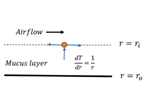
We assume a turbulent airflow shearing the mucus film, applicable to the proximal airways (Olson et al. Reference Olson, Sudlow, Horsfiel and Filley1973; Jain & Sznajder Reference Jain and Sznajder2007; Lin et al. Reference Lin, Tawhai, McLennan and Hoffman2007; Kleinstreuer & Zhang Reference Kleinstreuer and Zhang2009, Reference Kleinstreuer and Zhang2010; Xia et al. Reference Xia, Tawhai, Hoffman and Lin2010). It must be noted that the airflow in the proximal airways can remain turbulent or undergo transition even at a moderate Reynolds number due to the severe geometric transition in the proximal airways (Olson et al. Reference Olson, Sudlow, Horsfiel and Filley1973; Kleinstreuer & Zhang Reference Kleinstreuer and Zhang2009, Reference Kleinstreuer and Zhang2010). Here, we employ the locally Poiseuille model of Camassa & Lee (Reference Camassa and Lee2006) and Camassa et al. (Reference Camassa, Forest, Lee, Ogrosky and Olander2012). Thus the predictions of the present study could be improved further quantitatively by using the Camassa et al. (Reference Camassa, Ogrosky and Olander2014, Reference Camassa, Ogrosky and Olander2017) model. The consideration of the planar flow geometry by Patne (Reference Patne2022) was due to the small thickness of the saliva and mucus layers. Although planar flow geometry succeeds in capturing the effect of the shear-thinning and viscoelastic nature of the saliva and mucus on the dynamics, it removes the possibility of the existence of capillary or Plateau–Rayleigh instability that arises due to the azimuthal curvature coupled with air–mucus interface tension. Halpern & Grotberg (Reference Halpern and Grotberg1992), Halpern et al. (Reference Halpern, Fujioka and Grotberg2010), Zhou et al. (Reference Zhou, Peng, Zhang and Zhuge2014), Romano et al. (Reference Romano, Fujioka, Muradoglu and Grotberg2019, Reference Romano, Muradoglu, Fujioka and Grotberg2021) and Erken et al. (Reference Erken, Romano, Grotberg and Muradoglu2021) have illustrated the vital role played by the capillary instability in airway closure. Thus, to understand the impact of the inhaled air temperature on mucus dynamics, its effect on the elastic instabilities predicted by Patne (Reference Patne2022) and capillary instability predicted by Halpern & Grotberg (Reference Halpern and Grotberg1992), Halpern et al. (Reference Halpern, Fujioka and Grotberg2010), Zhou et al. (Reference Zhou, Peng, Zhang and Zhuge2014), Romano et al. (Reference Romano, Fujioka, Muradoglu and Grotberg2019, Reference Romano, Muradoglu, Fujioka and Grotberg2021) and Erken et al. (Reference Erken, Romano, Grotberg and Muradoglu2021) must be understood. To accomplish this, here we employ a cylindrical flow geometry with a turbulent airflow shearing a UCM liquid film lining the inner surface of the tube, as shown schematically in figure 1. To mimic the steam/cold air, the mucus layer is subjected to a radial heat flow.

Figure 1. Schematic of the model flow geometry in dimensionless coordinates. The airflow past the mucus layer leads to a flow and thermal energy exchange. For the inhalation of steam, the inhaled air temperature will be higher than the temperature of the muscles lined by the mucus, which leads to a radial heat flow across the mucus layer. In the case of cold-air inhalation, the opposite will be the case.
The rest of the paper is organised as follows. The base state, boundary conditions and perturbation governing equations are derived in § 2. The numerical methodology utilised here to solve the eigenvalue problem and its validation is presented in § 3. The analytical model based on the thin-film equation is formulated and discussed in § 4. The general linear stability analysis, i.e. stability analysis at arbitrary wavenumbers, and corresponding discussion are presented in § 5. The physical mechanism that leads to the thermocapillary induced stabilisation/destabilisation is discussed in § 6. Finally, the major conclusions obtained in the present study are presented in § 7.
2. Problem formulation
Here, we consider the model of Patne (Reference Patne2022) with the addition of the steam/cold-air-induced heat transfer and cylindrical flow geometry as shown schematically in figure 1. Consider an incompressible viscoelastic liquid layer of thickness  $2 R^*$, constant thermal conductivity $k^*_t$, thermal diffusivity $\alpha ^*$, dynamic viscosity $\mu ^*$, density $\rho ^*$, and shear modulus $G^*_f$. The assumption of a temperature-independent dynamic viscosity ( $\mu ^*$) will be justified in § 4. Here, $R^*=(r_o^* - r_i^*)/2$, with $r_i^*$ and $r_o^*$ the dimensional inner and outer radii of the airways. The inner radius $r_i^*$ is the distance from the centre of the airway to the air–mucus interface. The superscript ‘ $*$’ signifies a dimensional quantity. The turbulent air flowing past the liquid exerts a shear stress $\tau ^*_a$, which leads to a flow in the liquid layer with maximum velocity $V^*_m=-\tau ^*_a r^*_i \log (\beta )/\mu ^*$, where $\mu ^*$ is the viscosity of the liquid and $\beta =r_i^*/r_o^*$. The shear stress exerted by the air is defined by $\tau ^*_a = c^*_f \rho ^*_a V_a^{*2}/2$, with $c^*_f =0.02$, where $\rho ^*_a$ and $V_a^{*}$ are the density of the air and velocity of the air, respectively. The ratio of the gravity force on the film to the shear stress exerted by the turbulent airflow is $\rho ^* g^*/(\tau ^*_a/R^*) \ll 1$; thus the effect of gravity will be neglected in the subsequent analysis.
Muscles exhibit poor heat conduction (El-Brawany et al. Reference El-Brawany, Nassiri, Terhaar, Shaw, Rivens and Lozhken2009), so we neglect the heat dynamics in the muscles, and at  $r^*=r_o^*$ we assume a poor conducting solid. In such a setting, following Pearson (Reference Pearson1958) and Oron, Davis & Bankoff (Reference Oron, Davis and Bankoff1997), we assume that the liquid layer is subjected to a radial heat flow $\eta ^*$ in the $r$-direction. Also, we assume linear dependence of the surface tension ( $\varSigma ^*$) on the temperature of the interface ( $T^*$) (Pearson Reference Pearson1958; Oron et al. Reference Oron, Davis and Bankoff1997). Thus $\varSigma ^* = \varSigma _0^* - \gamma ^* (T^*-T_0^*)$, where $\varSigma _0^*$ is the air–liquid interface tension at the reference temperature $T_0^*$ and $\gamma ^* = -{{\rm d} \varSigma ^*}/{{\rm d} T^*}$.
The lengths, velocities and temperature are scaled by  $R^*$, $V^*_m$ and $\eta ^* R^*$, respectively. The pressure and stresses are non-dimensionalised by $\mu ^* V^*_m/R^*$. Let $T$ and $\boldsymbol {v}=(v_r,v_\theta,v_z)$ be the dimensionless temperature and velocity fields in the liquid, respectively. The scaled continuity, Cauchy momentum and energy equations are
 $$\begin{gather} \boldsymbol{\nabla}\boldsymbol{\cdot} \boldsymbol{v}=0, \end{gather}$$
 $$\begin{gather}Re \left[\frac{\partial \boldsymbol{v}}{\partial t}+(\boldsymbol{v}\boldsymbol{\cdot}\boldsymbol{\nabla}) \boldsymbol{v}\right]={-}\boldsymbol{\nabla} p + \boldsymbol{\nabla}\boldsymbol{\cdot}\boldsymbol{\tau}, \end{gather}$$
 $$\begin{gather}Re\,Pr \left[\frac{\partial T}{\partial t}+(\boldsymbol{v}\boldsymbol{\cdot}\boldsymbol{\nabla}) T \right]=\nabla^2 T, \end{gather}$$
where  $p$ is the pressure, $\boldsymbol {\tau }$ is the stress tensor, $Re=\rho ^* V^*_m R^*/\mu ^*$ is the Reynolds number, $Pr = \mu ^*/(\rho ^* \alpha ^*)$ is the Prandtl number, and $\boldsymbol {\nabla }$ is the gradient operator. To describe the dynamics of the mucus, we use the UCM model (Bird et al. Reference Bird, Armstrong and Hassager1977a; Larson Reference Larson1988)
 \begin{equation} \boldsymbol{\tau}+W \left[ \frac{\partial \boldsymbol{\tau}}{\partial t} + \boldsymbol{v} \boldsymbol{\cdot} \boldsymbol{\tau}- (\boldsymbol{\nabla}\boldsymbol{v})^{\rm T}\boldsymbol{\cdot} \boldsymbol{\tau}-\boldsymbol{\tau} \boldsymbol{\cdot} (\boldsymbol{\nabla}\boldsymbol{v}) \right]= \boldsymbol{\dot \gamma}, \end{equation}
where  $W=\lambda ^* V^*_m/ R^*$ is the Weissenberg number, with $\lambda ^*$ being the relaxation time, and $\boldsymbol {\dot \gamma }=(\boldsymbol {\nabla }\boldsymbol {v})+(\boldsymbol {\nabla }\boldsymbol {v})^{\rm T}$ is the strain-rate tensor.
At the dimensionless air–liquid interface  $r=r_i = 2\beta /(1-\beta )$, the above equations are supplemented with the kinematic boundary condition and the tangential and normal stress balance conditions. No-slip and impermeability conditions are applied at $r=r_o$, i.e. at the mucus–muscle interface. For the temperature field, at $r=r_i$, Newton's law of cooling is applied. At $r=r_o$, we assume a poor conducting substrate and impose a radial heat flow.
In the base state, the turbulent airflow is shearing the laminar mucus layer. For a steady-state, axisymmetric, fully developed base state, the quantities are (Miles Reference Miles1960; Smith & Davis Reference Smith and Davis1982; Patne Reference Patne2022)
 $$\begin{gather} \bar v_z = \frac{\log( r(1-\beta)/2 )}{\log(\beta)},\quad \frac{{\rm d}\bar T}{{\rm d} r} =\frac{1}{r}, \end{gather}$$
 $$\begin{gather}\bar \tau_{rz}=\frac{{\rm d} \bar v_z}{{\rm d} r},\quad \bar \tau_{zz}=2W \bar \tau_{rz}\,\frac{{\rm d} \bar v_z}{{\rm d} r}, \end{gather}$$
where an overbar signifies a base-state quantity. It must be noted that due to the azimuthal curvature effect, we impose a radial heat flow. As shown later, in § 4, in the lubrication approximation this corresponds to a constant temperature gradient across the mucus layer, corresponding to the earlier studies concerning thermocapillary instabilities in a liquid layer supported by a poorly conducting substrate (Pearson Reference Pearson1958; Patne, Agnon & Oron Reference Patne, Agnon and Oron2020b).
2.1. Linearised perturbation equations
To carry out the linear stability analysis, infinitesimally small perturbations are imposed on the base state (2.2). Owing to thermocapillarity and the cylindrical flow geometry, Squire's theorem is not applicable to the present system. Thus we consider non-axisymmetric perturbations. The governing equations (2.1) are linearised around the base state (2.2). In the linearised equations, normal modes of the form
 \begin{equation} f'(\boldsymbol{x},t)= \tilde f(r) \exp({{\rm i}(kz+n \theta -\omega t)}), \end{equation}
with  $f'(\boldsymbol {x},t)$ being the perturbation to a quantity and $\tilde f(r)$ the corresponding eigenfunction, are substituted. Here, $k$ and $n$ are the (real-valued) wavenumbers, while $\omega =\omega _r+{\rm i} \omega _i$ is the complex frequency of the disturbances. The flow is linearly unstable if at least one eigenvalue satisfies the condition $\omega _i>0$. Substitution of (2.3) into the linearised governing equations leads to
 $$\begin{gather} D \tilde v_{r}+\frac{\tilde v_{r}}{r}+\frac{{\rm i} n}{r}\,\tilde v_{\theta}+{\rm i}k \tilde v_{z}=0, \end{gather}$$
 $$\begin{gather}Re\,[{\rm i}\tilde v_{z} (k\bar v_{z}- \omega)+D \bar v_{z}\tilde v_{r}]={-}{\rm i}k\tilde p+{\rm i}k\tilde \tau_{zz}+D\tilde \tau_{rz} + \frac{1}{r}\,\tilde \tau_{rz} + \frac{{\rm i} n}{r}\, \tilde \tau_{\theta z}, \end{gather}$$
 $$\begin{gather}{\rm i}\,Re\,\tilde v_{r} (k\bar v_{z}-\omega) ={-}D\tilde p+{\rm i}k\tilde \tau_{rz}+D \tilde \tau_{rr} + \frac{1}{r}\,(\tilde \tau_{rz} - \tilde \tau_{\theta \theta}) + \frac{{\rm i} n}{r}\,\tilde \tau_{r \theta }, \end{gather}$$
 $$\begin{gather}{\rm i}\,Re\,\tilde v_{\theta} (k\bar v_{z}-\omega) ={-}\frac{{\rm i} n}{r}\,\tilde p+{\rm i}k\tilde \tau_{\theta z}+D\tilde \tau_{r\theta} + \frac{2}{r}\,\tilde \tau_{r\theta} + \frac{{\rm i} n}{r}\,\tilde \tau_{\theta \theta}, \end{gather}$$
 $$\begin{gather}Re\,Pr\,[{\rm i}\tilde T (k\bar v_{z}- \omega)+D \bar T\tilde v_{r}] = \left(D^2+\frac{1}{r}\, D-\frac{n^2}{r^2}-k^2 \right)\tilde T, \end{gather}$$
where  $D={\rm d}/{\rm d} r$. The constitutive equation (2.1d) gives
 \begin{gather} \tilde \tau_{zz} - {\rm i}\omega W \tilde \tau_{zz} + {\rm i} k W \tilde \tau_{zz} \bar v_z - 2 {\rm i} k W \bar \tau_{zz} \tilde v_{z} + W \tilde v_{r} D \bar \tau_{zz} - 2 W \tilde \tau_{rz} D \bar v_z \nonumber\\ -\,2 W \bar \tau_{rz} D \tilde v_{z} = 2 {\rm i} k \tilde v_{z}, \end{gather}
 \begin{gather} \tilde \tau_{rz} - {\rm i} \omega W \tilde \tau_{rz} - {\rm i} k W \bar \tau_{zz} \tilde v_{r} + {\rm i} k W \tilde \tau_{rz} \bar v_z - {\rm i} k W \bar \tau_{rz} \tilde v_{z} + W \tilde v_{r} D \bar \tau_{rz} \nonumber\\ -\,W \bar \tau_{rz} D \tilde v_{r} - W \tilde \tau_{rr} D \bar v_z = D \tilde v_{z} + {\rm i} k \tilde v_{r}, \end{gather}
 \begin{gather} \tilde \tau_{rr} - {\rm i} \omega W \tilde \tau_{rr} - 2 {\rm i} k W \bar \tau_{rz} \tilde v_{r} + {\rm i} k W \tilde \tau_{rr} \bar v_z = 2 D \tilde v_{r}, \end{gather}
 \begin{gather} \tilde \tau_{z \theta} - {\rm i} \omega W \tilde \tau_{z \theta} + \frac{W}{r}\,\bar \tau_{rz} \tilde v_{\theta} - {\rm i} k W \bar \tau_{zz} \tilde v_{\theta} + {\rm i} k W \tilde \tau_{z \theta} \bar v_z - W \bar \tau_{rz} D \tilde v_{\theta} \nonumber\\ -\,W \tilde \tau_{r \theta} D \bar v_z = \frac{{\rm i} n}{r}\,\tilde v_{z} + {\rm i} k \tilde v_{\theta}, \end{gather}
 $$\begin{gather} \tilde \tau_{r \theta} - {\rm i} \omega W \tilde \tau_{r \theta} - {\rm i} k W \bar \tau_{rz} \tilde v_{\theta} + {\rm i} k W \tilde \tau_{z \theta} \bar v_z = \frac{{\rm i} n}{r}\,\tilde v_{r} - \frac{1}{r}\,\tilde v_{\theta}+D \tilde v_{\theta}, \end{gather}$$
 $$\begin{gather}\tilde \tau_{\theta \theta} - {\rm i} \omega W \tilde \tau_{\theta \theta} + {\rm i} k W \tilde \tau_{\theta \theta} \bar v_z = \frac{2{\rm i} n}{r}\,\tilde v_{\theta} + \frac{2}{r}\,\tilde v_{r}. \end{gather}$$
 The above equations (2.4) are subject to the following boundary conditions. At the air–liquid interface, let the free surface be specified by  $r=r_i+h(z,\theta,t)$, where $h(z,\theta,t)$ is the displacement of the surface from the mean position $r=r_i$. At $r=r_i$, the kinematic boundary condition and the continuity of the tangential and normal stresses are imposed (Smith & Davis Reference Smith and Davis1982):
 $$\begin{gather} {\rm i}(k\bar v_z-\omega) \tilde h = \tilde v_r, \end{gather}$$
 $$\begin{gather}\tilde \tau_{rz}-2{\rm i}kW (D\bar v_z)^2 \tilde h={-}{\rm i}k\,Ma\, ( \tilde T - D \bar T \tilde h ), \end{gather}$$
 $$\begin{gather}\tilde \tau_{r\theta}={-}\frac{{\rm i}n}{r_i}\,Ma\,( \tilde T - D \bar T \tilde h), \end{gather}$$
 $$\begin{gather}-\tilde p + \tilde \tau_{rr} - 2{\rm i}k \bar \tau_{rz} \tilde h={-}\frac{1}{Ca} \left( \frac{1}{r_i^2}-k^2 - \frac{n^2}{r_i^2} \right) \tilde h, \end{gather}$$
 $$\begin{gather}D \tilde T + D^2 \bar T \tilde h + Bi\,\tilde T + Bi\,D \bar T \tilde h =0, \end{gather}$$
where  $h(z,\theta,t)=\tilde h \exp ({{\rm i} (kz+n \theta -\omega t)}), Ma={\gamma ^* \eta ^* R^*}/({\mu ^* V^*_m})$ is the Marangoni number, $Bi=q^* R^*/k^*_t$ is the Biot number with $q^*$ being the coefficient of heat convection or heat transfer coefficient, and $Ca=\mu ^* V^*_m/\varSigma _0^*$ is the capillary number. Referring to (2.2), a radially increasing base-state temperature gradient implies that the temperature at $r=r_o$ is higher than the temperature at $r=r_i$, for which $Ma>0$. At $r=r_o$, the muscle layer lined by the mucus is present. Thus the temperature at $r=r_o$ is the temperature of the muscles, which is the same as the body temperature, approximately $310$ K. Thus the $Ma>0$ scenario is possible when inhaled air is at a temperature lower than $310$ K. During inhalation of steam, the opposite is the case, so that $Ma<0$. At $r=r_o$, i.e. at the liquid–solid interface, we assume no-slip, impermeability and vanishing heat flux:
 \begin{equation} \tilde v_{r}=0, \quad \tilde v_{z}=0, \quad \tilde v_{\theta}=0, \quad D \tilde T=0. \end{equation}
 Next, the range of relevant parameters is estimated below. In the absence of respiratory diseases affecting the thickness of the mucus layer,  $r_i^* \sim r_o^*$ owing to the very small thickness of the mucus layer ( ${\sim } O(10^{-5})$ m), so $\beta \sim 1$ (Widdicombe & Widdicombe Reference Widdicombe and Widdicombe1995; Widdicombe Reference Widdicombe1997; Moriarty & Grotberg Reference Moriarty and Grotberg1999; Furlow & Mathisen Reference Furlow and Mathisen2018; Karamaoun et al. Reference Karamaoun, Sobac, Mauroy, Van Muylem and Haut2018). However, due to respiratory diseases, the thickness of the mucus layer could increase substantially, so that $\beta < 1$ (Shah et al. Reference Shah, Scott, Knight, Marriott, Ranasinha and Hodson1996; Moriarty & Grotberg Reference Moriarty and Grotberg1999). The mucus layer thickness decreases as one moves from the trachea to smaller units. The airway lumen also decreases correspondingly to approximately $250\,\mathrm {\mu }$m in the distal generation airways from 1 cm in the trachea; thus the $\beta$ value is maintained (Smith, Gaffney & Blake Reference Smith, Gaffney and Blake2008; Sanders et al. Reference Sanders, Rudolph, Braeckmans, De Smedt and Demeester2009; Karamaoun et al. Reference Karamaoun, Sobac, Mauroy, Van Muylem and Haut2018; Yi, Wang & Feng Reference Yi, Wang and Feng2021).
The density and viscosity of the mucus are of the order of  $10^{3}$ kg m $^{-3}$ and $10^{2}\unicode{x2013}10^{-3}$ Pa s, respectively, the air–mucus interface tension is of the order of $10^{-1}\unicode{x2013}10^{-2}$ N m $^{-1}$, the coefficient of heat convection is $q^* \sim 10\unicode{x2013}10^2$ W m $^{-2}$ K $^{-1}$, and $\gamma ^* \sim 10^{-5}\unicode{x2013}10^{-3}$ N m $^{-1}$ K $^{-1}$ (Hwang et al. Reference Hwang, Litt and Forsman1969; Li, Xu & Kumacheva Reference Li, Xu and Kumacheva2000; Schatz & Neitzel Reference Schatz and Neitzel2001; Lai et al. Reference Lai, Wang, Wirtz and Hanes2009; Hamed & Fiegel Reference Hamed and Fiegel2014; Hill et al. Reference Hill2014; Chen et al. Reference Chen, Zhong, Luo, Deng, Hu and Song2019). The exact value of $\gamma ^*$ for the mucus is unknown in the literature, so here we use the value for polymer solutions. The thermal conductivity of the mucus is of the order of $10^{-1}$ W m $^{-1}$ K (El-Brawany et al. Reference El-Brawany, Nassiri, Terhaar, Shaw, Rivens and Lozhken2009), and a typical temperature of the inhaled steam is 317–340 K (Singh et al. Reference Singh, Singh, Jaiswal and Chauhan2017), with body temperature 310 K, and $\eta R \sim O(10)$.
The mean velocity of the exhaled air is  $V^*_a \sim 1\unicode{x2013}10$ m s $^{-1}$ (Moriarty & Grotberg Reference Moriarty and Grotberg1999; Tang et al. Reference Tang, Nicolle, Pantelic, Koh, Wang and Amin2012; Geoghegan et al. Reference Geoghegan, Laffra, Hoogendorp, Taylor and Jermy2017), while normal breathing velocity in the proximal airways is $V^*_a \sim 1$ m s $^{-1}$ (Lin et al. Reference Lin, Tawhai, McLennan and Hoffman2007). It must be noted that as the air travels to the higher generations of airways, the velocity decreases; thus the velocity is approximately $3$ m s $^{-1}$ in the trachea, but much lower in the later generations of the airways. Also, the airflow is turbulent in the proximal airways and laminar in the higher-generation airways (Lin et al. Reference Lin, Tawhai, McLennan and Hoffman2007; Kleinstreuer & Zhang Reference Kleinstreuer and Zhang2009, Reference Kleinstreuer and Zhang2010; Xia et al. Reference Xia, Tawhai, Hoffman and Lin2010). For a turbulent airflow, we use the formula $\tau ^*_a = c^*_f \rho ^*_a V_a^{*2}/2$ with $c^*_f =0.02$ to obtain $V^*_m \sim 10^{-2}\unicode{x2013}10^{-6}$ m s $^{-1}$ (Miesen & Boersma Reference Miesen and Boersma1995). The order of magnitude of the dimensionless parameters is given in table 1. From table 1, the Reynolds number is $Re \ll 1$ and the Biot number is $Bi \ll 1$; thus we consider the creeping-flow limit, i.e. $Re=0$ and $Bi=10^{-5}$, in the following discussion.
Table 1. Orders of magnitude of the dimensionless parameters using the dimensional parameters.

3. Numerical methodology
To solve the eigenvalue problem (2.4) subject to the boundary conditions (2.5), we employ the pseudo-spectral method. In this method, the eigenfunctions for each dynamic field are expanded into a series of Chebyshev polynomials as
 \begin{equation} \tilde{f}(\kern0.7pt y)=\sum_{m=0}^{m=M} a_m\,\mathcal{T}_m (\kern0.7pt y), \end{equation}
where  $\mathcal {T}_m(\kern0.7pt y)$ are Chebyshev polynomials of degree $m$, and $M$ is the highest degree of the polynomial in the series expansion or, equivalently, the number of collocation points. The series coefficients $a_m$ are the unknowns to be solved for. The generalised eigenvalue problem is constructed in the form
 \begin{equation} \boldsymbol{A}\boldsymbol{e} + \omega \boldsymbol{B}\boldsymbol{e} =0, \end{equation}
where  $\boldsymbol {A}$ and $\boldsymbol {B}$ are the discretised matrices and $\boldsymbol {e}$ is the vector of $a_m$.
The details of the discretisation procedure and construction of the matrices can be found in Trefethen (Reference Trefethen2000) and Schmid & Henningson (Reference Schmid and Henningson2001). We use the eig MATLAB routine to solve the eigenvalue problem (3.2). To filter out the spurious modes from the genuine, numerically computed spectrum of the problem, the latter is determined for  $N$ and $N+2$ collocation points, and the eigenvalues are compared with an a priori specified tolerance, e.g. $10^{-4}$. The genuine eigenvalues are verified by increasing the number of collocation points by $25$ and monitoring the variation of the obtained eigenvalues. Whenever the eigenvalue does not change up to a prescribed precision, e.g. to the sixth significant digit, the same number of collocation points is used to determine the critical parameters of the system. The above-described numerical methodology has been utilised previously to solve similar problems by Patne & Shankar (Reference Patne and Shankar2020), Patne, Agnon & Oron (Reference Patne, Agnon and Oron2020a), Patne et al. (Reference Patne, Agnon and Oron2020b), Patne, Agnon & Oron (Reference Patne, Agnon and Oron2021a,Reference Patne, Agnon and Oronb), Patne & Oron (Reference Patne and Oron2022) and Patne (Reference Patne2022).
Next, we use two-way validation for the present numerical methodology. First, to validate the numerical methodology for the azimuthal curvature, the closest flow geometry is the sliding Couette flow in which the airflow region will be replaced by a moving rigid cylinder. Thus the sliding Couette flow and present flow geometry will differ only in the boundary conditions at  $r=r_i$, while the rest of the quantities will remain the same (Patne & Shankar Reference Patne and Shankar2020). Since previous studies of Preziosi & Rosso (Reference Preziosi and Rosso1990), Deguchi & Nagata (Reference Deguchi and Nagata2011) and Liu & Liu (Reference Liu and Liu2012) considered the sliding Couette flow of a Newtonian liquid, here we consider $W=0$. Table 2 shows excellent agreement between the present numerical methodology and previous studies for the least stable eigenvalue, thereby validating the numerical methodology utilised in the present work.
Table 2. A comparison of the least stable eigenvalue reported in the previous studies and predictions obtained from the present numerical method for the sliding Couette flow of a Newtonian liquid ( $W=0$). The excellent agreement between the previous studies and present numerical method predictions validates the latter.

To validate further the present numerical methodology, we compare the most unstable eigenvalue predicted by Patne (Reference Patne2022) and that obtained from the present numerical methodology. It must be noted that Patne (Reference Patne2022) considered a planar flow geometry, while here we have a cylindrical flow geometry; thus the predictions of Patne (Reference Patne2022) could be reproduced using the present geometry provided that  $\beta \rightarrow 1$ for an axisymmetric mode. Furthermore, Patne (Reference Patne2022) used the WM model to describe the dynamics of the mucus layer and the neo-Hookean model for the muscles lined by the mucus layer. These factors can be removed by neglecting the shear-rate dependence of the viscosity and relaxation time, solvent contribution to the viscosity, and deformability of the muscles. Thus, for ease of comparison, we use the unity power-law index, vanishing solvent contribution, and $\varGamma =0$ in the model of Patne (Reference Patne2022), where $\varGamma$ signifies the deformability of the muscles. A finite air–mucus interface tension leads to an additional capillary instability in the cylindrical flow geometry considered here (Halpern & Grotberg Reference Halpern and Grotberg1992; Zhou et al. Reference Zhou, Peng, Zhang and Zhuge2014; Erken et al. Reference Erken, Romano, Grotberg and Muradoglu2021); therefore in the comparison we have used $Ca = \infty$, and same has been implemented in the model of Patne (Reference Patne2022). Additionally, we have considered $Ma=0$, thereby neglecting the effect of air temperature. After using these modifications, the most unstable eigenvalue predicted by the present numerical methodology and that given by the Patne (Reference Patne2022) model exhibit good agreement at low wavenumber $k$, as shown in table 3, thereby validating the former. However, as $k$ increases, the disagreement between the eigenvalues increases. This discrepancy arises because the lubrication approximation (and hence the planar flow assumption) fails to work for high $k$. This conclusion can be drawn from the thin-film analysis carried out in § 4.
Table 3. A comparison of the most unstable eigenvalue for the planar flow case studied by Patne (Reference Patne2022) and predicted by the present study at  $W=0.1$ and $Re=0$. For ease of comparison, the White & Metzner (Reference White and Metzner1963) liquid considered in the analysis of Patne (Reference Patne2022) is reduced to a UCM model by considering the unity power-law index, vanishing solvent contribution, and absence of the deformable muscles supporting the mucus layer (i.e. $\varGamma =0$). To facilitate comparison with the planar flow geometry, we have performed calculations for the axisymmetric mode at $\beta =0.99$ and $Ca = \infty$ in the present flow. The effect of the azimuthal curvature becomes dominant as $k$ increases, hence the difference in the eigenvalues for the planar flow case studied by Patne (Reference Patne2022) and the present study.

4. Thin-film analysis
The capillary and elastic modes of instability are long-wave, i.e. they exhibit instability for  $k < 1$. Therefore, the simplest way to analyse the impact of thermocapillarity induced by inhaled air temperature is to understand its effect on the long-wave instabilities. Additionally, as noted above, for a healthy human adult, $\beta \rightarrow 1$ because of the very small thickness of the mucus layer. Owing to these circumstances, in this section we carry out the thin-film analysis.
As will be shown later, in § 5, the axisymmetric mode is the most unstable mode; thus here we consider the same. We will develop a simple model along the lines of Patne (Reference Patne2022). It must be noted that the following derivation is applicable strictly in the linear limit. Following Halpern & Grotberg (Reference Halpern and Grotberg1992), we use the transformation  $r^*=r^*_o - y^*$, where $y^*$ is a new coordinate that is appropriate for considering a thin annular film. Now, scaling $r^*$ by $r^*_o$ and $y^*$ by $R^*$ leads to $r=1-\epsilon y$ such that $r_o=1$ and $r_i=1-\epsilon$, implying the mucus domain transformation from $r \in [r_i,r_o]$ to $y \in [1,0]$. Here, $\epsilon = R^*/r^*_o \ll 1$ is a small parameter. Also, $t \rightarrow t/\epsilon$ and $z \rightarrow Z/\epsilon$. Using these scalings, the governing equations (2.1) are modified. Next, we substitute the following expansions into the modified equations:
 $$\begin{gather} v_z = \bar v_z + \epsilon v'_z + \cdots,\quad v_r = \epsilon^3 v'_r + \cdots,\quad p = \frac{1}{\epsilon^2}\,p' + \cdots, \end{gather}$$
 $$\begin{gather}\tau_{rz} = \frac{1}{\epsilon}\,\bar \tau_{rz} + \tau'_{rz} + \cdots,\quad \tau_{zz} = \frac{1}{\epsilon}\,\bar \tau_{zz} + \tau'_{zz} + \cdots,\quad \tau_{rr} = \epsilon \tau'_{rz} + \cdots, \end{gather}$$
 $$\begin{gather}\tau_{\theta \theta} = \epsilon \tau'_{\theta \theta} + \cdots . \end{gather}$$
 The above procedure applied to (2.1) at  $O(1)$ gives
 \begin{equation} \frac{\partial \bar \tau_{rz}}{\partial y} = 0,\quad \bar \tau_{rz} ={-}\frac{\partial \bar v_z}{\partial y},\quad \bar \tau_{zz} ={-}2 W \bar \tau_{rz}\,\frac{\partial \bar v_z}{\partial y} = 2 W \left(\frac{\partial \bar v_z}{\partial y}\right)^2, \quad \frac{\partial^2 \bar T}{\partial y^2} = 0, \end{equation}
where we have used the transformation  $W \rightarrow \epsilon W$, thereby restricting the analysis to low $W$. Solving the above equations for the base-state velocity and temperature profile leads to
 \begin{equation} \bar v_z = y, \quad \bar T = C-y, \end{equation}
where  $C$ is an unspecified dimensionless integration constant. In the lubrication approximation, the mucus layer is subjected to the base-state temperature gradient, ${\partial \bar T}/{\partial y}=-1$. The linear stability of the above base-state velocity profile in the absence of warm air has been studied in detail by Patne (Reference Patne2022).
At this stage, the assumption of a temperature-independent viscosity could be justified as follows. Following Char & Chen (Reference Char and Chen2014), we employ a Nahme-type relationship to relate viscosity and temperature:
 \begin{equation} \mu^* = \mu^*_0 \exp({-A^* (T^*-T_r^*)}), \end{equation}
where  $T_r^*$ is the reference temperature at which $\mu ^* = \mu ^*_0$. The dimensional temperature field in the lubrication approximation is $T^*=C^* - \eta ^* y^*$, where $\eta ^*$ is the imposed temperature gradient and $C^*$ is the dimensional integration constant. Substituting this into the above equation, we obtain
 \begin{equation} \mu^* = \mu^*_0 \exp({-A^* (C^* - \eta^* y^* - T_r^*)}). \end{equation}
Assuming that the reference temperature is selected such that  $T_r^* = C^*$ leads to
 \begin{equation} \mu^* = \mu^*_0 \exp({A^* \eta^* y^*}). \end{equation}
The imposed temperature gradient is  $\eta ^* =-{{\rm d} \bar T^*}/{{{\rm d}y}^*} \sim (T^*(\kern0.7pt y^*=0) - T^*(\kern0.7pt y^*=R^*))/ {R^*}$. In the case of steam inhalation, $T^*(\kern0.7pt y^*=R^*) > T^*(\kern0.7pt y^*=0)$. Let ${\rm \Delta} T^* = T^*(\kern0.7pt y^*=R^*) - T^*(\kern0.7pt y^*=0)$; then for steam inhalation, $\eta ^* \sim -{{\rm \Delta} T^*}/{R^*}$. Substituting this into (4.8) leads to
 \begin{equation} \mu^* \sim \mu^*_0 \exp\left({-A^*\,\frac{{\rm \Delta} T^*\,y^*}{R^*}}\right). \end{equation}
 Char & Chen (Reference Char and Chen2014) define a dimensionless variable  $B = A^*\,{\rm \Delta} T^* = \ln (\mu ^*_{max}/\mu ^*_{min})$. Now substituting $A^* = {B}/{{\rm \Delta} T^*}$ into (4.9) gives
 \begin{equation} \mu^* \sim \mu^*_0 \exp\left({-B\,\frac{y^*}{R^*}}\right). \end{equation}
Thus the difference between the viscosities at the mucus–muscle interface ( $y^*=0$) and the air–mucus interface ( $y^*=R^*$) is of the order of $\mu ^*_0 (1 - {\rm e}^{-B} )$. Char & Chen (Reference Char and Chen2014) consider $B \sim O(0\unicode{x2013}10)$. It must be noted that they considered such a high value of $B$ because their study involved buoyancy convection in addition to thermocapillary convection and was thus applicable to thick liquid layers. In the present study, we are concerned with only thermocapillary convection for which the liquid layer under consideration is $O(10^{-5})$ m; thus the $B$ value will be substantially lower for the present study, implying that the difference between the viscosities at the mucus–muscle interface and the air–mucus interface will also be low. Therefore we neglect the temperature dependence of the viscosity in the present study.
At  $O(\epsilon )$, the governing equations (2.1) give
 $$\begin{gather} -\frac{\partial \tau'_{rz}}{\partial y} - \frac{\partial p'}{\partial Z} = 0, \end{gather}$$
 $$\begin{gather}\tau'_{rz} ={-}\frac{\partial v'_z}{\partial y}. \end{gather}$$
In the perturbed state, let the air–mucus interface be  $y=1-\zeta$, with $\zeta$ the deflection from the mean position $y=1$. The boundary conditions become
 $$\begin{gather} v'_z = 0 \quad \text{at}\ y=0, \end{gather}$$
 $$\begin{gather}\frac{\partial v'_z}{\partial y} - 2 W\,\frac{\partial \zeta}{\partial Z} = Ma\,\frac{\partial \zeta}{\partial Z} \quad \text{at}\ y=1, \end{gather}$$
 $$\begin{gather}p' ={-}\frac{1}{Ca}\left[\frac{\partial^2 \zeta}{\partial Z^2} +\zeta\right] \quad \text{at}\ y=1, \end{gather}$$
where the transformations  $Ma \rightarrow Ma/\epsilon$ and $Ca \rightarrow \epsilon ^{3}\,Ca$ have been used to retain the Marangoni and capillary terms.
Solving (4.11) gives
 \begin{equation} v'_z = (Ma + 2 W) y\,\frac{\partial \zeta}{\partial Z} + ( y + 2 \zeta-2)\,\frac{y}{2}\,\frac{\partial p'}{\partial Z}. \end{equation}
The kinematic boundary condition at  $O(\epsilon )$ is
 \begin{equation} \frac{\partial \zeta}{\partial t} + \frac{\partial \zeta}{\partial Z} + \frac{\partial}{\partial Z} \int_0^{1} v'_z \,{{\rm d}y}=0. \end{equation}
Substituting (4.12) into the above equation yields the linear equation
 \begin{equation} \frac{\partial \zeta}{\partial t} + \frac{\partial \zeta}{\partial Z} + \frac{\partial}{\partial Z} \left[ \left( W +\frac{Ma}{2} +\frac{1}{3\,Ca} \right) \frac{\partial \zeta}{\partial Z} +\frac{1}{3\,Ca}\,\frac{\partial^3 \zeta}{\partial Z^3} \right]=0. \end{equation}
Substituting  $\zeta = \tilde \zeta \exp ({{\rm i}(k Z-\omega t)})$ into the above equation and solving for $\omega$ gives
 \begin{equation} \omega = k + {\rm i} k^2 \left( W +\frac{Ma}{2} +\frac{1}{3\,Ca} \right) - \frac{{\rm i}k^4}{3\,Ca}. \end{equation}
Thus, for the long-wave perturbations to be stable,  $Ma<0$ and $|Ma|>2[W+1/(3\,Ca)]$, implying that the thermocapillarity stresses caused by the inhaled steam can suppress the elastic and capillary instabilities in the airways. In the opposite scenario involving cold-air inhalation, $Ma > 0$, so the thermocapillarity will enhance the instabilities.
The dispersion relation (4.15) could be extended easily to include the solvent effect by noting the change in the elastic term, which arises due to the first normal stress difference across the mucus–air interface. In the presence of the solvent, from Patne (Reference Patne2022),  $\bar \tau _{zz} = 2 (1-\beta _s) W ({\partial \bar v_z}/{\partial y})^2$, where $\beta _s$ is the ratio of the solvent viscosity to the solution viscosity. Thus, in the presence of the solvent, the above dispersion relation becomes
 \begin{equation} \omega = k + {\rm i} k^2 \left( (1-\beta_s) W +\frac{Ma}{2} +\frac{1}{3\,Ca} \right) - \frac{{\rm i}k^4}{3\,Ca}.\end{equation}
From this equation, consideration of the solvent reduces the destabilising influence of the viscoelastic nature of the mucus. Thus the elastic mode will be stabilised at a lower  $Ma$.
$Ma$.
Given the assumptions made in deriving (4.15), it should be readily applicable to the planar flow model of Patne (Reference Patne2022). Hence we next compare predictions of (4.15) and Patne (Reference Patne2022) by modifying the original isothermal model of the latter to include the heat transfer induced by the inhaled air temperature. This modification entails an additional energy equation, and the mucus layer is subjected to a normal temperature gradient  ${\rm d} \bar T/{{\rm d}y} = -1$ in the base state. Furthermore, the WM model used in his study is reduced to the UCM model by assuming the unity power-law index, vanishing solvent contribution, and absence of the deformable muscles supporting the muscle layer. Figure 2 shows that for $W=0.1$, $Ma=-0.2$ is necessary to stabilise the elastic instability, while for $W=0.5$ the necessary condition is $Ma=-1$. This indicates that $Ma<0$ and $|Ma|>2W$ are necessary to suppress the elastic mode, in excellent agreement with predictions of (4.15). It must be noted that owing to the absence of the azimuthal curvature, the capillary mode cannot be captured by using the Patne (Reference Patne2022) model.

Figure 2. The effects of variation in  $Ma\ (<0$) on the elastic mode using the modified Patne (Reference Patne2022) model at $Ca=1$, $\beta =0$ and $Re=0$ for a UCM liquid: (a) $W=0.1$, (b) $W=0.5$. The figure validates the inequality $|Ma|>2W$ to suppress the elastic mode suggested by (4.15).
5. General linear stability analysis
The analysis in § 4 is restricted to a small wavenumber limit owing to the thin-film approximation. In this section, we analyse the stability of arbitrary wavenumber disturbances. For convenience of presentation, the discussion is divided into three sections.
5.1. Elastic modes
Patne (Reference Patne2022) predicted the existence of a purely elastic mode of instability when the mucus is sheared by an isothermal airflow. His analysis showed further that the elastic mode arises due to the first normal stress difference across the air–mucus interface, a characteristic of a viscoelastic liquid. He assumed a planar flow geometry to model the airflow in the oral cavity and airways owing to the small thickness of the mucus and saliva layers. To accommodate the capillary instability relevant in the airways owing to their tubular structure, here we consider a cylindrical flow geometry. This could also lead to additional non-axisymmetric modes of instability and the effect of azimuthal curvature. Thus, next, we discuss the effects of azimuthal curvature and non-axisymmetry on the purely elastic mode predicted by Patne (Reference Patne2022).
Variation in the azimuthal curvature is represented by the parameter  $\beta =r^*_i/r^*_o$. Thus as the thickness of the mucus layer increases, $\beta$ decreases. Figure 3(a) shows the stabilising effect of increasing azimuthal curvature on the axisymmetric mode. Similarly, figure 3(b) shows the unstable axisymmetric and non-axisymmetric modes. It must be noted that for a Newtonian liquid in the vanishing interface tension limit (i.e. $Ca=\infty$), the axisymmetric mode is linearly stable, while the non-axisymmetric modes will be linearly stable for arbitrary interface tension. However, from figure 3(b), both axisymmetric and non-axisymmetric modes are unstable even in the vanishing air–mucus interface tension limit, with the former possessing a higher growth rate than the non-axisymmetric modes. This implies that the first normal stress difference across the air–mucus interface destabilises axisymmetric and non-axisymmetric modes.

Figure 3. The effects of variation in azimuthal curvature  $\beta$ and azimuthal wavenumber $n$ on the purely elastic mode at $k=0.5$, $Ca=\infty$, $W=0.5$ and $Ma=0$. (a) Plot for $n=0$; here, $\beta$ has been decreased from $0.9$ to $0.3$ in steps of $0.1$ with the points having the highest and lowest $\omega _i$ values belonging to $\beta =0.9$ and $\beta =0.3$, respectively. Thus, as the azimuthal curvature effect increases, i.e. as $\beta$ decreases, the growth rate of the purely elastic mode decreases. (b) Plot for $\beta =0.9$; here, $n=0$ and $n=4$ correspond to the points with the highest and lowest $\omega _i$ values, and $n$ has been increased in steps of $1$. Thus, the axisymmetric ( $n=0$) elastic mode possesses a higher growth rate than non-axisymmetric ( $n \neq 1$) elastic modes.
Having identified the axisymmetric mode as the most unstable mode, next we analyse the impact of steam inhalation on this mode. Figure 4 shows the strong stabilising effect of the thermocapillarity on the elastic mode, with complete stabilisation at a certain value of  $Ma$ (depending on $\beta$) provided that $Ma<0$. The inequality $Ma<0$ implies that the inhaled air must be at a higher temperature than the muscle layers lined by the mucus, i.e. body temperature, which is indeed the case with steam inhalation. Since the growth rate of the elastic mode decreases with decreasing $\beta$, a lower value of $|Ma|$ is necessary to stabilise the elastic mode at low $\beta$.

Figure 4. Dispersion curves for  $Ma<0$ on the axisymmetric mode at $Ca=\infty$, $Bi=10^{-5}$ and $W=0.1$: (a) $\beta =0.8$, (b) $\beta =0.9$. We consider $Ma<0$ for steam inhalation since the mucus layer surface will be at a higher temperature than the muscles lined by the mucus. The thermocapillarity induced by the inhaled steam stabilises the elastic instability successfully.
5.2. Capillary mode
Apart from the elastic mode, the other important mode of instability is the capillary or Plateau–Rayleigh mode, which arises due to the tendency of the liquid to minimise the surface area (Halpern & Grotberg Reference Halpern and Grotberg1992; Zhou et al. Reference Zhou, Peng, Zhang and Zhuge2014; Romano et al. Reference Romano, Fujioka, Muradoglu and Grotberg2019, Reference Romano, Muradoglu, Fujioka and Grotberg2021; Erken et al. Reference Erken, Romano, Grotberg and Muradoglu2021). Furthermore, unlike the elastic mode predicted by Patne (Reference Patne2022), the capillary mode exhibits a higher growth rate with decreasing  $\beta$. Thus for high $\beta$, the elastic instability dominates, while for low $\beta$, capillary instability dominates the stability of the flow. For example, at $\beta =0.98$, $W=0$, $Ma=0$, $k=0.01$ and $Ca=0.0001$, the capillary mode is $\omega = 0.009895002 + 1.098818 \times 10^{-5}{\rm i}$, while the elastic mode at $\beta =0.98$, $W=1$, $Ma=0$, $k=0.01$ and $Ca=\infty$ is $\omega =0.009892367 + 9.842448 \times 10^{-5}{\rm i}$. It must be noted that we have used extreme values of $Ca$ and $W$ despite the fact that the elastic mode exhibits a higher growth rate than the capillary mode.
Since  $\beta <1$ during the common cold, due to the increased thickness of the mucus layer, the capillary instability will become severe as the intensity of the common cold increases, which could lead to airway closure as predicted in the previous studies of Halpern & Grotberg (Reference Halpern and Grotberg1992), Zhou et al. (Reference Zhou, Peng, Zhang and Zhuge2014), Romano et al. (Reference Romano, Fujioka, Muradoglu and Grotberg2019, Reference Romano, Muradoglu, Fujioka and Grotberg2021) and Erken et al. (Reference Erken, Romano, Grotberg and Muradoglu2021). Thus for steam inhalation to work effectively, it should be able to stabilise the capillary mode also. Figure 5 shows that, indeed, the thermocapillary effect induced by the steam can also stabilise the capillary mode successfully. It must be noted that from the literature (Drazin & Howard Reference Drazin and Howard1966; Drazin Reference Drazin2002), any non-axisymmetric capillary mode will be stable, so those modes are not included in the discussion.

Figure 5. Dispersion curves for selected values of  $Ma$ on the capillary mode at $Ca=0.01$, $Bi=10^{-5}$ and $W=0$: (a) $\beta =0.8$, (b) $\beta =0.9$. The figure illustrates that the capillary mode is stabilised successfully by thermocapillarity.
5.3. Elasto-capillary mode
From the above discussion, for non-zero  $W$ and finite $Ca$, the axisymmetric mode can become unstable due to the elasticity (via first normal stress difference) and capillarity at the air–mucus interface. These two destabilisation mechanisms are different and so could lead to two different unstable modes or merge and give rise to a single, more powerful unstable mode. From figure 6, the present flow system follows the latter mechanism. The elastic mode at $W=0.5$, $Ca=\infty$, $\beta =0.9$ and $k=0.05$ is $\omega = 0.046806 + 1.1098 \times 10^{-3}{\rm i}$, while the capillary mode at $W=0$, $Ca=0.01$, $\beta =0.9$ and $k=0.05$ is $\omega = 0.046881 + 3.8466 \times 10^{-4}{\rm i}$. A comparison of these two eigenvalues shows that the $\omega _r$ values for both modes are approximately equal, but the $\omega _i$ values differ. Thus the elasticity and capillarity destabilise the perturbations of nearly the same frequency. For $W=0.5$, $T=10$, $\beta =0.6$ and $k=0.05$, the two modes merge to give rise to a single mode, $\omega = 0.046791 + 1.4936 \times 10^{-3}{\rm i}$, henceforth referred to as the ‘elasto-capillary mode’. The elastic, capillary and elasto-capillary modes are shown in figure 6. The elasto-capillary mode has a growth rate equal to the combined growth rate of the elastic and capillary modes and has frequency approximately the same as both modes.

Figure 6. The axisymmetric elastic, capillary and elasto-capillary modes at  $Ma=0$, $\beta =0.8$ and $k=0.05$. The elastic mode is for $W=0.5$ and $Ca=\infty$; the capillary mode is for $W=0$ and $Ca=0.01$; and the elasto-capillary mode is for $W=0.5$ and $Ca=0.01$. The elastic and capillary modes merge to give the elasto-capillary mode, which possesses a growth rate nearly equal to the sum of the growth rates of the individual elastic and capillary modes.
It must be noted that the elasto-capillary mode presented here is not the same as the ‘resonance mode’ predicted by Patne (Reference Patne2022), which arises due to the resonance between the liquid and solid elastic modes. The resonance mode had a considerably higher growth rate than the sum of the growth rates of the liquid and solid elastic modes. However, the elasto-capillary mode predicted here has a growth rate nearly equal to the sum of the growth rates of the elastic and capillary modes, as depicted in figure 6.
From the predictions of Patne (Reference Patne2022), the elasticity of the muscles lined by the mucus will also play a vital role in reinforcing the elastic mode predicted here. Thus the elasticity of the mucus and underlying muscles could lead to the elasticity-dominated elasto-capillary mode, which could induce finite-amplitude oscillations in the mucus layer. In the case of decreasing  $\beta$ due to pulmonary diseases, the elastic mode will exhibit a lower growth rate, but the capillary mode becomes severe; thus the capillarity becomes dominant in the elasto-capillary mode. To conclude, both the elasticity (of the mucus and underlying muscles) and the capillarity could play a major role in destabilising the mucus layer.
The elasto-capillary mode, similar to the elastic and capillary modes, is stabilised by the thermocapillarity induced by the steam, as shown in figure 7, albeit at a higher  $|Ma|$ than the individual elastic (see figure 4) and capillary (see figure 5) modes. Furthermore, due to finite $Ca$, compared with the elastic mode for which $Ca=\infty$, the elasto-capillary mode is constrained to a lower $k$ range.

Figure 7. The effects of variation in  $Ma$ on the axisymmetric elasto-capillary mode at $Ca=0.01$, $Bi=10^{-5}$ and $W=0.5$: (a) $\beta =0.8$, (b) $\beta =0.9$. The thermocapillarity induced by the steam stabilises the elasto-capillary mode successfully.
So far, we have discussed the stabilising effect of the thermocapillary stresses caused by steam inhalation, which implies  $Ma<0$. The case with $Ma>0$ is possible when the inhaled air is colder than the human body temperature. Figure 8 predicts a destabilising influence of an increasing positive $Ma$ on the mucus layer. Thus cold air leads to enhancement of the hydrodynamic instabilities.

Figure 8. The effects of variation in  $Ma>0$ on the axisymmetric mode at $Ca=0.1$, $Bi=10^{-5}$ and $W=0.5$: (a) $\beta =0.8$, (b) $\beta =0.9$. As $Ma$ increases, the growth rate of the elasto-capillary mode increases rapidly, thereby implying a destabilising effect of the thermocapillarity.
6. Physical mechanism
The analysis of Patne (Reference Patne2022) showed that the first normal stress difference across the air–mucus interface is responsible for the elastic instability predicted here, while the capillary instability arises due to the tendency of a liquid to minimise the surface area (Drazin Reference Drazin2002). The physical mechanism of the onset of Marangoni convection in a static liquid layer subjected to a wall-normal temperature gradient can be found in the literature (Smith & Davis Reference Smith and Davis1983a,Reference Smith and Davisb; Patne et al. Reference Patne, Agnon and Oron2021a). For a Newtonian liquid layer ( $W=0$) subjected to a wall-normal temperature gradient, the thermocapillary convection arises due to the Marangoni stresses acting at the air–liquid interface, as seen from (4.11d):
 \begin{equation} \frac{\partial v'_z}{\partial y}=Ma\,\frac{\partial \zeta}{\partial Z}. \end{equation}
The results predicted in the present study arise due to the competition between the elasticity of the mucus, air–mucus interface tension, and thermocapillarity induced by the inhaled air. While the elasticity and capillarity always have a destabilising effect on the mucus layer, from § 5, the thermocapillarity could have a stabilising or destabilising effect depending on the temperature of the inhaled air. The aim of this section is to explain the process by which the thermocapillarity induced by the inhaled steam leads to the suppression of the elastic and capillary instabilities, which could lead to the observed therapeutic effect of steam inhalation in patients.
At the mucus–air interface, due to the viscoelasticity of the mucus, (6.1) becomes
 \begin{equation} \frac{\partial v'_z}{\partial y}-2W\,\frac{\partial \zeta}{\partial Z}=Ma\, \frac{\partial \zeta}{\partial Z}. \end{equation}
Thus, in the absence of the thermocapillary stresses (i.e.  $Ma=0$), owing to the base-state first normal stress difference across the air–mucus interface (term $-2W ({\partial h}/{\partial Z})$), there is an ‘extra tangential stress’ acting on the air–mucus interface. This extra tangential stress then leads to the development of the perturbations, thereby leading to the predicted instability (Brady & Carpen Reference Brady and Carpen2002). Similarly, to destabilise the air–mucus interface, the capillarity will help in growing the peak of a pressure perturbation wave since the thickness of the mucus layer is larger than the mean thickness $r_o^* - r_i^*$ at the peak through a decreased pressure due to interface tension. For the trough, the opposite scenario is applicable, thereby reinforcing the trough. The increasing pressure perturbations will assist in the growth of the longitudinal velocity perturbations via the momentum equations. Thus both the elasticity of the mucus and the capillarity at the air–mucus interface enhance the peak in the longitudinal velocity perturbation wave.
If we switch on the thermocapillarity, then  $Ma\neq 0$, and from the interface condition (6.2), growing longitudinal velocity perturbations will help in the growth of the thermal perturbations. This is when the sign of $Ma$ comes into play. First, consider the case of steam inhalation for which $Ma<0$, implying a positive radial heat flow imposed on the mucus layer.
Consider a random peak in the thermal perturbations, which is being forced to grow by the longitudinal velocity perturbations due to coupling through interface condition (6.2). A peak in the thermal perturbations at the interface corresponds to a region possessing a temperature higher than that of the surrounding fluid, as shown schematically in figure 9. Due to thermocapillarity, such a peak will have a surface tension lower than that of the surrounding fluid. Thus there will be a flow of fluid from the peak towards the adjacent troughs, which will be at a lower temperature. From mass balance, this flow at the interface will be compensated by the flow of mucus from the layers below the interface. Such a flow will be opposed by the viscous forces in the mucus. Since there is a positive radial heat flow imposed on the mucus layer (i.e.  $T|_{r=r_i} > T|_{r=r_o}$), the mucus flowing towards the peak will be at a lower temperature than the mucus present at the interface. Thus the mucus reaching the peak through the flow will try to cool down the temperature peak. At the same time, the temperature peak will also lose energy by thermal diffusion. These two mechanisms eventually suppress the temperature peak, thereby stabilising the thermal perturbations. This stabilising effect on the thermal perturbations spreads to the longitudinal velocity perturbations via interface condition (6.2) and perturbations to other dynamic quantities to eventually stabilise the latter. This results in the predicted stabilising effect of the thermocapillarity on the elastic and capillary instabilities in the airways.

Figure 9. A schematic of a hot spot generated randomly due to thermal perturbations. The arrows indicate the direction of the thermocapillary flow. At the interface, the thermocapillary flow will be away from the hot spot because of the surface tension gradient. To fill this mass drainage, there will be a colder mucus flow from the inside of the mucus layer to the air–mucus interface, which will stabilise the elasto-capillary mode.
In the absence of the thermocapillarity, the growing perturbations could eventually grow to a finite-amplitude wave and invade the airway lumen space (Halpern & Grotberg Reference Halpern and Grotberg1992; Grotberg Reference Grotberg2001; Romano et al. Reference Romano, Fujioka, Muradoglu and Grotberg2019; Erken et al. Reference Erken, Romano, Grotberg and Muradoglu2021). The invasion of the airway lumen reduces the area for airflow, thereby leading to an increase in airway resistance. The thermocapillary stabilisation introduced through the inhaled steam removes the very instabilities responsible for the growth of the perturbations. Thus the thermocapillarity could help in reducing the airway resistance to the airflow, thereby leading to the observed therapeutic effect of steam inhalation.
If we inhale colder air, then  $Ma>0$. Thus there will be an opposite effect, and the temperature peak (hence the longitudinal velocity perturbation peak), which is growing due to the elasticity and capillarity effects, will be further forced to grow due to the thermocapillarity, thereby increasing the severity of the airway instabilities. This, in turn, could lead to an increase in airway resistance, in agreement with observations of Fontanari et al. (Reference Fontanari, Burnet, Zattara-Hartmann and Jammes1997).
6.1. Effect of viscosity variation with temperature
The effect of variation in viscosity due to temperature on the results predicted here could be understood as follows. From the above discussion, the thermocapillarity exerts a stabilising/destabilising influence through the tangential stress balance condition at the air–mucus interface (i.e. at  $r^*=r_i^*$), which in dimensional form for a Newtonian fluid is
 \begin{equation} \frac{\partial v^*_z}{\partial r^* } + \frac{\partial v^*_r}{\partial z^* } ={-} \frac{\gamma^*}{\mu^*}\,\boldsymbol{\nabla}^* T^* \boldsymbol{\cdot} \boldsymbol{t}, \end{equation}
where  $\boldsymbol {t}$ is the unit tangent vector at the air–mucus interface and $\gamma ^* = -{{\rm d} \varSigma ^*}/{{\rm d} T^*}$. For the steam inhalation case, the temperature will increase at the air–mucus interface. Thus, from the above discussion, the viscosity of the mucus $\mu ^*$ will decrease correspondingly. This decrease in the viscosity, from (6.3), while other parameters are kept constant, will lead to an enhancement of the thermocapillary effect. Thus if we consider the temperature dependence of the viscosity in the present study, then the elasto-capillary mode will be stabilised at a lower Marangoni number $Ma$. Physically, this could be seen as the existence of a lesser viscous resistance to the colder mucus that is trying to flow from inside of the layer to the hot spot shown in figure 9 at the air–mucus interface due to a decreasing viscosity as we approach the air–mucus interface. This lesser resistance leads to enhanced cooling of the hot spot, thereby enhancing the effect of the steam inhalation. The opposite will be the case if the inhaled air temperature is lower than the body temperature.
7. Summary
The present study deals with linear stability analysis of a viscoelastic liquid layer lining the inside of a tube subjected to a wall-normal constant radial heat flow and sheared by turbulent airflow. We propose this as a model to understand the effect of steam/cold-air inhalation on mucus dynamics.
The present analysis reveals the existence of non-axisymmetric elastic modes along with the axisymmetric mode, with the latter exhibiting a higher growth rate than the former. Also, an increasing azimuthal curvature, characterised by the decreasing of the parameter  $\beta$, is predicted to have a stabilising effect on the elastic modes. Thus the elastic mode predicted in the previous study of Patne (Reference Patne2022), by assuming a planar flow geometry owing to the small thickness of the mucus layer, predicted the most unstable elastic mode. The elastic modes arise due to the first normal stress difference in the base state across the air–mucus interface. Thus the driving force for the elastic mode is the base flow induced by the turbulent airflow.
Steam inhalation imposes a positive radial heat flow across the mucus layer, implying a Marangoni number  $Ma<0$. The stability analysis carried out here predicts a successful stabilisation of the elastic mode by the thermocapillarity induced by the inhaled steam. Furthermore, as $\beta$ decreases, the $|Ma|$ value required for stabilising the elastic mode decreases.
Previous studies of Halpern & Grotberg (Reference Halpern and Grotberg1992), Erken et al. (Reference Erken, Romano, Grotberg and Muradoglu2021), Romano et al. (Reference Romano, Fujioka, Muradoglu and Grotberg2019, Reference Romano, Muradoglu, Fujioka and Grotberg2021) and Zhou et al. (Reference Zhou, Peng, Zhang and Zhuge2014) predicted the existence of the capillary mode in the airways. In healthy human beings  $\beta \rightarrow 1$, but diseases affecting the mucus layer will give $\beta <1$. The growth rate of the capillary mode increases with increasing azimuthal curvature; thus, normally, in the absence of diseases leading to an increase in the thickness of the mucus layer, the capillary mode will be subdominant while the elastic mode will be the dominant one. The analysis shows that the capillary mode could also be stabilised by the thermocapillarity for $Ma<0$, i.e. if the inhaled air temperature exceeds the body temperature.
The elastic mode of Patne (Reference Patne2022) and the capillary modes merge to give rise to the elasto-capillary mode, which has a growth rate approximately equal to the combined growth rate of the elastic and capillary modes. The elasto-capillary mode, by virtue of having a higher growth rate, requires a higher  $|Ma|$ for its successful stabilisation than the individual elastic and capillary modes. Furthermore, $Ma>0$, corresponding to the inhaled air possessing a temperature lower than the body temperature, leads to an increase in the growth rate of the elasto-capillary mode.
The physical mechanism of the stabilisation/destabilisation due to the thermocapillarity is explained in § 6. The analysis shows that inhaled steam decreases airway resistance during breathing. Additionally, steam also leads to a decrease in the viscosity of the mucus, thereby helping the mucus clearance mechanism. An opposite scenario emerges when the inhaled air is colder than the body temperature, which leads to an increase in airway resistance during breathing, in agreement with the observations of Fontanari et al. (Reference Fontanari, Burnet, Zattara-Hartmann and Jammes1997). A simple thin-film model in the linear limit is derived, which affirms the numerical predictions.
In the present study, we have assumed a turbulent airflow relevant to the proximal airways, while the higher-generation airways will have a laminar airflow (Lin et al. Reference Lin, Tawhai, McLennan and Hoffman2007; Xia et al. Reference Xia, Tawhai, Hoffman and Lin2010). However, the capillary instability predicted in the previous studies (and also here) will be still relevant because of the azimuthal curvature effect at the air–mucus interface. Similarly, elastic instability will also be present since it arises due to the first normal stress difference across the air–mucus interface, which remains true even for a laminar airflow past a mucus layer. Thus the elasto-capillary mode predicted in the present study will also be present in the higher-generation airways, albeit with a quantitative adjustment to the growth rate. The effect of thermocapillarity could be reduced due to the loss of thermal energy by the air while reaching the higher-generation airways. To conclude, even for the higher-generation airways where laminar airflow exists, the present analysis can provide a qualitative picture of the instabilities and their suppression by the thermocapillarity due to steam inhalation.
We conjecture further that the inhaled steam could also help in depositing water in the mucus layer, which will increase the proportion of the solvent, thereby decreasing the concentration of the mucin and non-mucin protein macromolecules that are responsible for the rheological properties of the mucus (Basser, McMahon & Griffith Reference Basser, McMahon and Griffith1989; Wu & Carlson Reference Wu and Carlson1991; Lai et al. Reference Lai, Wang, Wirtz and Hanes2009; Lafforgue et al. Reference Lafforgue, Seyssiecq-Guarante, Poncet and Favier2017). The decrease in the protein concentration leads to a corresponding decrease in the viscosity and relaxation time; thus the mucus offers less resistance to the flow and decreases the Weissenberg number  $W$. The viscosity of the mucus could also decrease due to the high temperature of the steam, commonly observed for polymer solutions (Bird et al. Reference Bird, Armstrong and Hassager1977a; Bird, Armstrong & Hassager Reference Bird, Armstrong and Hassager1977b). A decreasing viscosity thus could enhance the removal of the mucus from lungs by a mucus clearance mechanism, in agreement with observations (Singh et al. Reference Singh, Singh, Jaiswal and Chauhan2017). This particular feature could play a big role in diseases that lead to an increase in the viscosity of the mucus, such as cystic fibrosis (Shah et al. Reference Shah, Scott, Knight, Marriott, Ranasinha and Hodson1996). A decreasing $W$ helps in decreasing the severity of the elastic instability. Thus steam inhalation could achieve a therapeutic effect by suppressing the elastic and capillary instabilities exhibited by the mucus layer and decreasing the viscosity.
Thus the present analysis answers the questions about the effect of inhaled steam/cold air on the mucus layer dynamics in the airways. However, the present study deals only with linear stability analysis. A complete nonlinear analysis would give a much clearer picture of the capability of the inhaled steam in altering the mucus dynamics. The present study could also be extended to distal airways where the airflow is laminar. Additionally, in vitro experiments could be carried out to validate the predictions of the present study.
Funding
The author acknowledges financial support from the Indian Institute of Technology Hyderabad, India, under grant SG/IITH/F280/2022-23/SG-118.
Declaration of interests
The author reports no conflict of interest.


