


Introduction
Surge behaviour is characterized by cyclical instabilities related to internal changes in the glacier system rather than external factors such as climate change (Reference Meier and PostMeier and Post, 1969), although the mechanism responsible for surge behaviour is still debated. Two major mechanisms have been proposed, one involving a thermal trigger (e.g. Reference SchyttSchytt, 1969; Reference ClarkeClarke, 1976) and one involving subglacial hydrology (e.g. Reference Clarke, Collins and ThompsonClarke and others, 1984; Reference KambKamb and others, 1985). Glacier dynamics, not only during the surge phase, but also during the quiescent phase, are of importance in understanding surge behaviour.
Svalbard is an Arctic archipelago, of which about 60% is covered by glaciers (Reference Hagen, Liestøl, Roland and JørgensenHagen and others, 1993). The Svalbard glaciers are classified as polythermal (Reference SchyttSchytt, 1969; Bjo¨rns-son and others, 1996). It is assumed that at least 13% (Reference Jiskoot, Boyle and MurrayJiskoot and others, 1998) and up to 90% (Reference LiestølLiestøl, 1988) of these glaciers are of the surge type. Recently it has been suggested that some Svalbard glaciers, with known surges in the past, are no longer building up to new surges (Reference Dowdeswell, Hodgkins, Nuttall, Hagen and HamiltonDowdeswell and others, 1995). This is supposed to be a result of climate warming in the Arctic, after the termination of the Little Ice Age about 100 years ago.
This paper investigates whether or not Hessbreen is building up towards a new surge. We also take a brief look at what the present glacier dynamics can indicate about the initiation processes of the last surge, as well as presenting new data from this surge. We will focus on the quiescent phase of Hessbreen, and the transition from the quiescent state to the surge state.
Field Area
Hessbreen is a small valley glacier in southern Spitsbergen (778300 N, 158060 E), situated a few kilometres west of the larger Finsterwalderbreen (Fig. 1). Reference HambergHamberg (1905) first mapped the area in 1898. Since then, several aerial photographs (1936, 1956, 1969, 1970, 1990, 1995) at scales of 1 :17000 to 1 : 50 000 that cover parts of the glacier have been taken for the Norwegian Polar Institute. The glacier is now about 5 km long and terminates at a large push moraine. The accumulation area is up to 2.25km wide, but the glacier narrows sharply to <1 km below 300ma.s.l. Hessbreen faces northeast and is surrounded by high mountains. The upper area is divided into basins by a nunatak, and the equilibrium-line altitude (ELA) is assumed to be at 330 m a.s.l. (Reference Hagen, Liestøl, Roland and JørgensenHagen and others, 1993). At present, crevasses are almost absent except for some small areas close to the nunatak and in the transition to ice aprons. Comparison of air photos from 1936 and 1956 shows that the degree of crevassing then and now is quite similar. The area considered here is 5.1 km2, which covers Hessbreen up to 600m a.s.l., although there are ice aprons extending along the back wall to an elevation of 950 m a.s.l.

Fig. 1. Location map of Svalbard with insert of Hessbreen/Finster-walderbreen.
Hessbreen is classified as a polythermal glacier by Reference LiestølLiestøl (1976), based on the existence of water drainage during wintertime and temperature measurements. The glacier is known to have surged during 1972–76 (Reference LiestølLiestøl, 1976; Reference Dowdeswell, Hamilton and HagenDowdeswell and others, 1991) and probably also surged just before 1900, as in 1898 the glacier front was against the outermost moraine (Reference HambergHamberg, 1905). The bedrock in the area consists of soft sedimentary rocks (Reference DallmannDallmann and others, 1990; Reference HjelleHjelle, 1993). Such conditions are considered, by some glaciologists, to be relevant to surges (e.g. Reference Clarke, Collins and ThompsonClarke and others, 1984; Reference Jiskoot, Boyle and MurrayJiskoot and others, 1998).
Methods
Radio-echo soundings
Multi-frequency radio-echo sounding (RES) data were collected along the centre line and two cross-sections in spring 1995 (Fig. 2). The time-gated synthetic pulse radar system is described in Reference Hamran, Gjessing, Hjelmstad and AarholtHamran and others (1995), and measurements conducted at Finsterwalderbreen at the same time and with the same equipment are discussed thoroughly in Ødega__rd and others (1997). Along the centre line, both 30–80MHz end-fed broad-bandwidth dipole antennae and 320–370 MHz six-element Yagi antennae were used. For cross-sections B–B’ and C–C’ (Fig. 2), only 30–80 MHz were used. C–C’ is close to the ELA cross-section which is used for the balance-flux calculation. The radio-echo soundings are combined with the elevation contours based on aerial photos from 1990 (unpublished map from A. J. Fox, 1995).
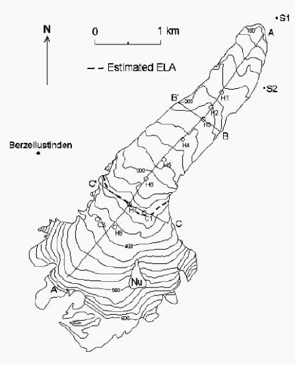
Fig. 2. Location of stakes H1–H8, C1 and C3, reference points S1 and S2, RES profiles A–A′, B–B′ and C–C′ and estimated ELA (350 m). Based on map by A. J. Fox (unpublished data). Elevation contours in m a.s.l. with 20 m intervals. Nu is a nunatak.
The radio-echo soundings were carried out 5 years after the aerial photography, but no significant change in the glacier surface in this period is assumed.
Surveying
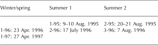
The surveying was based on ten stakes (Fig. 2). During spring 1994, two velocity stakes, H2 and H6, were installed on the centre line of the glacier. This line was supplemented with six more stakes in summer 1995. The total length of this transect was about 2.5 km. Two more stakes, C1 and C3, were added east and west respectively of the two uppermost stakes. These stakes were meant to form a transect with H7 in the centre, but C3 had to be moved due to the large amount of rocks being incorporated into the ice below the mountain, Berzeliustinden (Fig. 2). Two reference points, S1 and S2 (Fig. 2), were established on the end moraine and a hill east of the glacier. Both sites were vegetated and it was assumed that the points were sufficiently stable for this relatively short period of survey. A cairn on the island Eholmen, about 9.8 km northwest of the end moraine, was used as a reference target in the surveying. The stakes were surveyed using a theodolite (Wild T2) and an EDM (Wild Di3000), most being observed from both fixed points S1 and S2. The measurements were made six times between summer 1995 and spring 1997, and dates are listed in Table 1. Due to fog, it was impossible to measure all stakes during each survey.
Table 1. Surveying sessions of Hessbreen and their corresponding dates
Mass balance
The winter balance was measured along the stake profile. Due to a lack of stakes, the coverage above the ELA was poor (Fig. 2). As a supplement to the Hessbreen measurements, the results were compared with data from Finsterwalder-breen (Fig. 3), which has an intermittent mass-balance series from 1950 (Reference LiestølLiestøl, 1976; Reference Nuttall, Hagen and DowdeswellNuttall and others, 1997). Over the last 50years, there has been no significant trend in the total net mass-balance data. The mass-balance data of Finsterwalderbreen have been applied to Hessbreen.

Fig. 3. Left scale: area distributions of Hessbreen and Finsterwalder-breen. Right scale: observed winter snow depth for 1994, 1995 and 1996. The data for 1994 and 1996 are sparse and shown only as points.
Basal shear stress and dynamic balance
The basal shear stress τ is given by
(Reference NyeNye, 1965), where ρ is the density of ice, g the gravitational constant, h the ice thickness and α the surface slope. Nye introduced the shape factor f to give a more realistic estimate of the shear stress in valley glaciers. f is a dimensionless parameter that varies with the geometry of the glacier. The difference between the balance and the dynamic fluxes at a given horizontal location x along the glacier gives the rate of mass increase above x.
where M (x) is the mass above the position x, Q b (x) is the balance flux across the section and Q v (x) the volume flux or the actual flux across the section (e.g. Reference Raymond and ColbeckRaymond, 1980). Here Q b is approximated as
where A is the upstream area of the section x, and b is th average net balance in this area. The volume flux Q v is her approximated by:
where ![]() is the annual surface velocity in the middle of the section and S the area of the section.
is the annual surface velocity in the middle of the section and S the area of the section.
Results and Interpretation
Thermal regime and influence on the drainage pattern
The RES shows the interface between cold and temperate ice up to about 4 km up-glacier from the terminus. This assumption is made from interpretation of radio-echo measurements with the same equipment as on Finster-walderbreen (Reference Hamran, Gjessing, Hjelmstad and AarholtHamran and others, 1995) and other Svalbard glaciers (Reference BjörnssonBjörnsson and others, 1996). However, reflections from the bed could be followed only 2.5 km up-glacier (Fig. 4c). Interpretation of the longitudinal transect is shown in Figure 5, and suggests that the glacier is at the pressure-melting point over most of the bed along the centre line, with the exception of the lower ~600 m. The first few hundred metres of the 320-370 MHz profile (Fig. 4d) did not agree with the 30-80MHz profile (Fig. 4c), probably due to englacial material in this area.
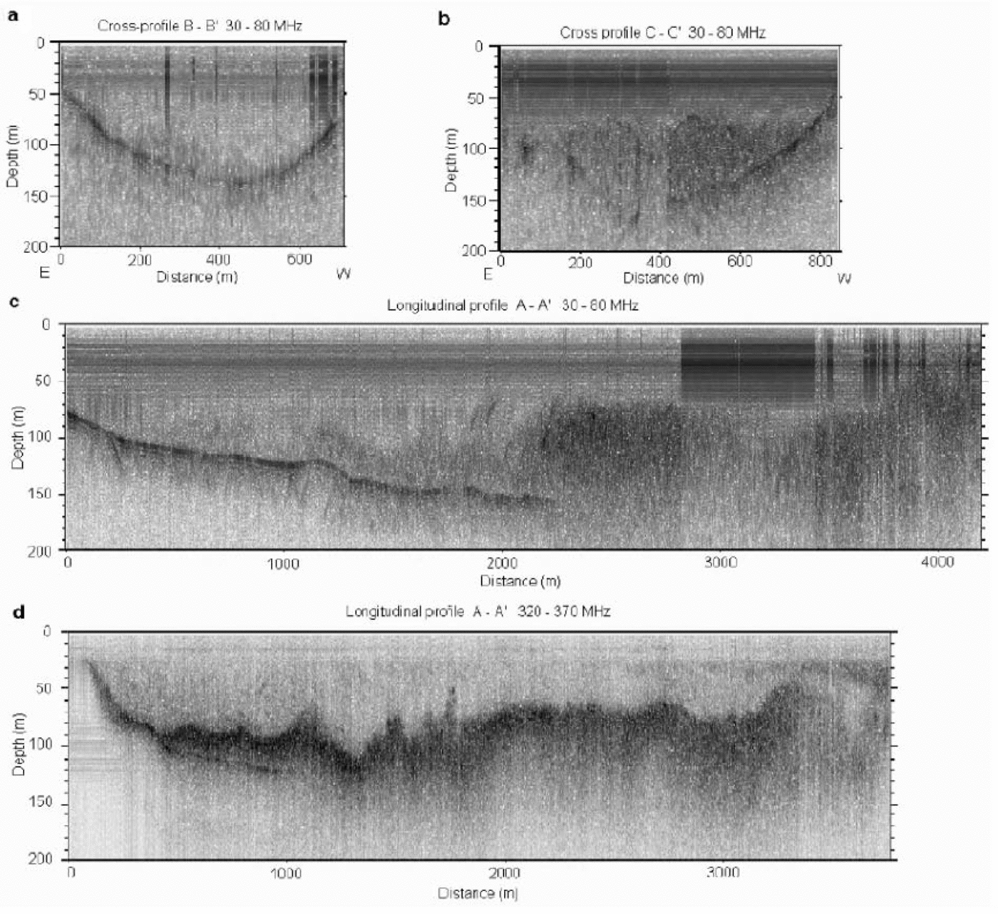
Fig. 4. RES profile images. Cross sections B–B′ (a) and C–C′ (b) and longitudinal profile (c) show the ice depth, and longitudinal profile (d) indicates the thickness of the cold surface layer. The longitudinal profiles start about 300 m from the glacier front.
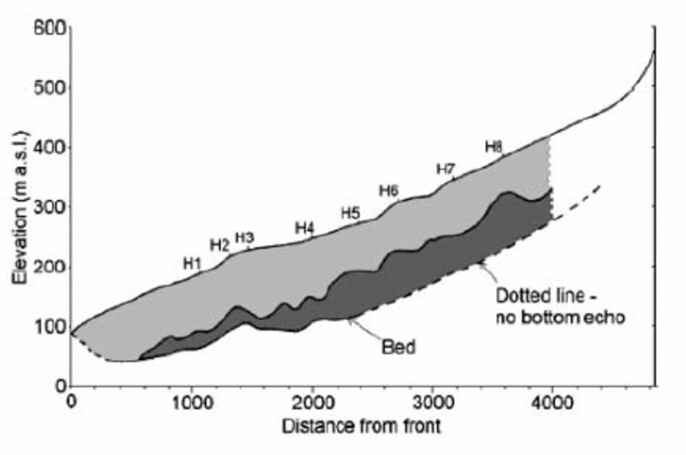
Fig. 5. Interpretation of the radio-echo profiles. Light raster indicates cold ice, darker raster temperate ice. Surface profile drawn from map (A. J. Fox, unpublished data). Surveying stakes H1–H8 are marked. Missing data near the front and lack of bottom echo are drawn with dotted line.
As few crevasses are present, glacier meltwater drains mainly supraglacially in a network, with the channels developing in the central part of the glacier. In the lower part, the main channels end in moulins. In the 1995 photos the pattern and location of several of the channels were similar to those appearing in the 1956 photos. Icing in front of the glacier was observed during this study and could also be seen on the air photos.
Flow velocities
The survey data were calculated as stake coordinates using a least-squares solution with both direction and distance measurements. The accuracy, given as standard deviation of the stakes coordinates, was ±0.03 to ±0.1 m. This is rather high, but not unexpected due to the often difficult observation conditions. Direction measurements are more influenced by difficult conditions than distances, and the velocity results have been based on distance measurements only. The direct distance measurements from the fixed point S1, which are more or less exactly in line with the glacier flow, were used to calculate stake velocities, except for stakes H4 and H5 where distances measured from the fixed point S2 were used. From S2 these distance measurements have angles to the flowline of approximately 17° and 21°, which have been taken into account. Velocities from the direct distance measurements correspond well (most within 10%) with velocities computed from the adjusted coordinates. The surface velocities along the centre line and cross-profile are shown in Figure 6 and Table 2. The vectors of ice movement are shown in Figure 7.
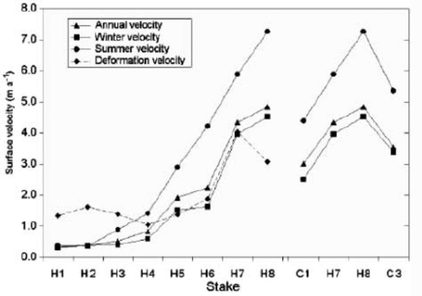
Fig. 6. Surface velocities at stakes: annual, winter and summer.
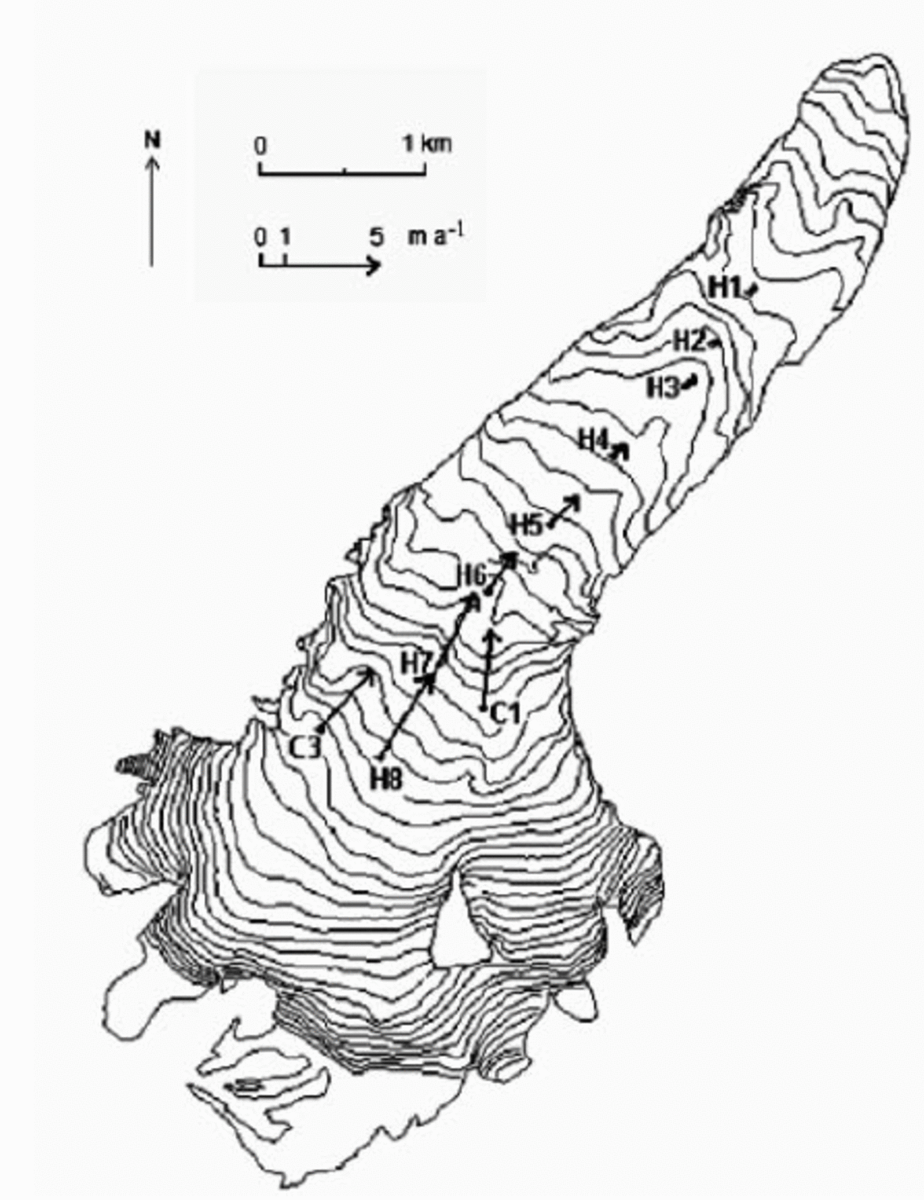
Fig. 7. Velocity and direction of ice movement at stakes (annual mean values).
Table 2. Measured velocities and corresponding standard deviations (sdev) of stakes. Annual (A), winter (W) and spring/summer or summer velocities (S) and their standard deviations. Units are m a-1
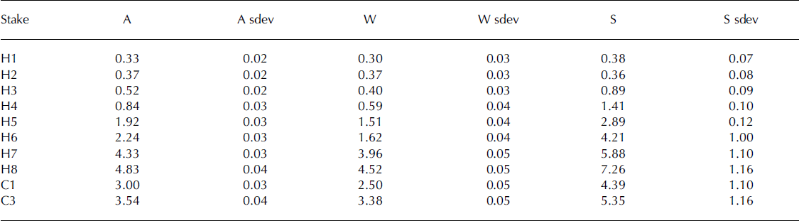
The annual velocities are calculated for the period 2-95 to 3-96 (349 days; see Table 1). The interval between 2-95 and 1-96 forms the basis of the winter velocities (245 days). For some of the stakes, winter velocities can also be computed for the period 2-96 to 1-97 (263 days), but due to melting out and tilting of some stakes these results have not been used except to verify the listed results. The two winter velocities coincidewithin±0.1 m a-1 for stakes H1-H3, and ±0.2 m a-1 for stakes H6-H8. The summer velocities can be calculated between 1-95 and 2-95 (11 days), or 2-96 and 3-96 (20 days), but measurements are not available for all stakes in both the periods. The time-spans are very short and the estimated standard deviations of the velocity vectors are as high as or even higher than the velocities found for the slowest-moving stakes. The summer velocities of stakes H1-H5 have thus been computed as the combined spring/summer velocity in 1996 (1-96 to 3-96), as there was no significant difference between the spring and summer velocities for these stakes. The velocities and their corresponding standard deviations are listed in Table 2. Forall stakes, the annual velocities were close to their winter velocities, which were 71-95% of the annual velocity. The increased summer velocities can only last for 1-3 months to achieve the observed annual velocities. The largest seasonal variation was found at stake H6, where the summer velocity was 2.6 times the winter velocity. The velocities probably fluctuate during the spring/summer season, with velocities both higher and lower than the estimated averages of this season.
Basal shear stress
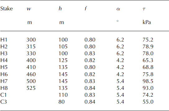
The RES profiles (Fig. 4a and b) confirm the assumption that the cross-profile approximates a semi-ellipsoid. Values of the shape factor f for semi-ellipsoidal profiles (Reference NyeNye, 1965) vary between 0.80 and 0.84 (Table 3). The surface slopes were calculated by averaging over 8-10 times the average ice thickness at each stake (Reference Meier, Kamb, Allen and SharpMeier and others, 1974), and vary between 4.28 and 6.28. The basal shear stress τ (Equation (1)) was calculated from measured elevation profiles and f values. τ was highest at stake H7, with a maximum value of 99kPa, decreasing to a minimum of 65 kPa at stake H4, and increasing again at stake H3.
Table 3. Values used for calculation of basal shear stress τ. w is the half-width, h the centre-line depth, f the shape factor and α the surface slope
Mass balance
The net mass-balance results from 1994 to 1996 (Table 4), which had warmer than average summers, showed the ELA of Hessbreen to be approximately 400 m a.s.l. Reference Hambrey and DowdeswellHambrey and Dowdeswell (1997) also found the limit of superimposed ice in 1995 to be at about 400 m a.s.l. The ELA of Finsterwalder-breen in these years was found to be at 500 m a.s.l. (Reference Nuttall, Hagen and DowdeswellNuttall and others, 1997), about 100 m higher than the 50 year average (Reference Hagen, Liestøl, Roland and JørgensenHagen and others, 1993). The mass balance is stable in this area, and generally correlates well with the ELA (e.g. Reference YoungYoung, 1981; Reference Hagen and LiestølHagen and Liestøl, 1990). The ELA at Hessbreen has been estimated before at 330 m a.s.l. (Reference Hagen, Liestøl, Roland and JørgensenHagen and others, 1993), based upon stake measurements from the 1970s and related to the ELA at Finsterwalderbreen (personal communication from O. Liestøl, 1999). It is thus assumed that the average ELA at Hessbreen is no higher than 350m a.s.l. (Fig. 2) and probably slightly lower.
Table 4. Net mass balance for Finsterwalderbreen (F) and Hessbreen (H), 1995 and 1996
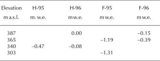
The comparison between the mass balances of Hessbreen and Finsterwalderbreen (Fig. 3) shows slightly higher accumulation on Hessbreen, which could be due to local topography. The more shaded location of Hessbreen could account for there being less ablation, and accumulation from avalanches is probably more important for the mass balance of the small Hessbreen than for the larger Finsterwalderbreen. Other investigations have shown that superimposed ice is common on Svalbard glaciers (Reference LiestølLiestøl, 1974, and on Finsterwalderbreen this represents a significant portion of the total accumulation (Ødega__rd and others, 1997; inglot and others, 1997) which is also true for Hessbreen. The water equivalent data for Finsterwalder-breen (Reference Nuttall, Hagen and DowdeswellNuttall and others, 1997) are used in the calculations for Hessbreen, assuming that this will give slightly lower values than the actual situation on Hessbreen. If a build-up situation is found with these lower mass-balance values, it will strengthen the probability of an actual build-up on Hessbreen.
Surge history
Reference LiestølLiestøl (1976) assumed that the last surge of Hessbreen started between 1972 and 1974. However, aerial photos from late August 1969 (NP S69 2905–2908 and S69 2965– 2967, approximate scale 1 : 17 000) show long, transverse, crescent-shaped crevasses in the upper part of the glacier and down to about 300m a.s.l., and also lateral crevasses further down along the eastern side (Fig. 8). These are not visible on other aerial photos, except on those from 1970 (scale 1 :50000), and are not described earlier. Liestøl reported no visible crevasses on a visit to the glacier at 520 m a.s.l. in early summer 1968 (personal communication from O. Liestøl, 1999), which suggests that the surge was initiated between Liestøl’s visit and the aerial photography, i.e. between the summers of 1968 and 1969. As no crevassing was observed towards the snout of the glacier during a survey of the lower part in 1972, there was a delay before the surge became fully developed.
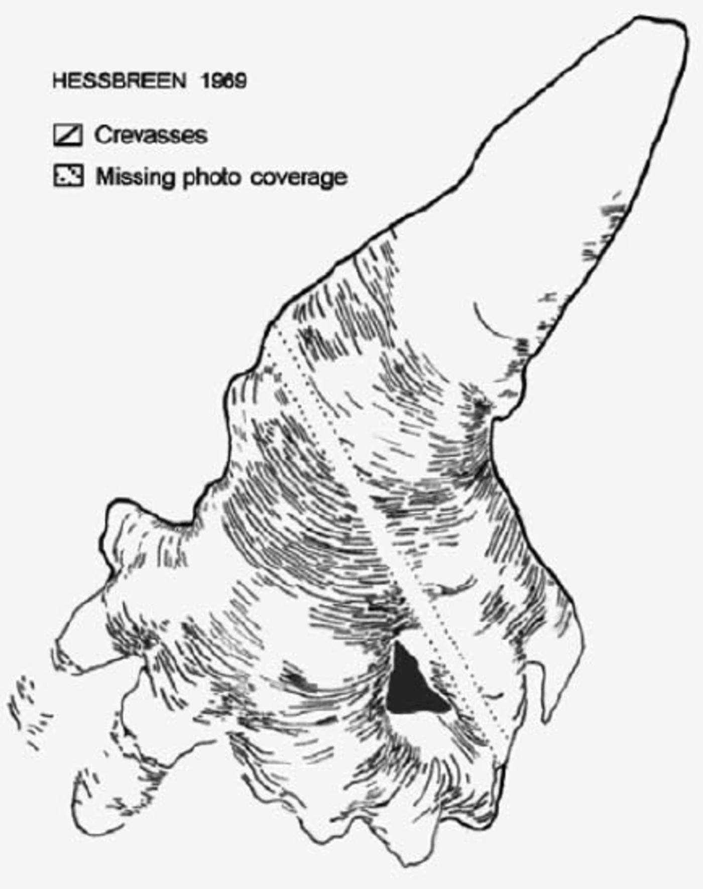
Fig. 8. Crevasse pattern from aerial photos NP S69 2905–2908 and S69 2965–2967. The crevasses outside the outline indicate crevassing in the ice aprons. Note: figure has incorrect map geometry.
Discussion
Thermal regime and drainage
In small or narrow polythermal glaciers the glacier bed is cold and the glacier is frozen to the bedrock (Bjo¨nsson and others, 1996). A ‘cold ring thermal regime’, with cold, ‘dry’ ice uppermost and surrounding temperate, ‘wet’ ice in the inner zones, is found in several glaciers on Svalbard (e.g. Reference SchyttSchytt, 1969; Reference Kotlyakov and MacheretKotlyakov and Macheret, 1987). From the RES data only, it is difficult to determine whether the low velocities at the snout are caused by cold ice throughout or if temperate ice in the centre is strongly influenced by cold marginal ice. Ice velocities in the narrow part of the glacier show a fall instead of the expected increase. The decrease in velocity from the upper to the lower stakes can partly be explained by the decrease in ice thickness. The shape of structures from former crevasses (aerial photos NP S95 1121–1123), and avalanche patterns on the glacier surface indicate the presence of cold marginal ice. Whilst the crevasse traces are straight and parallel in the upper-middle part, those further downstream near the glacier terminus have a sharp, convex down-glacier profile. This study suggests that Hessbreen has a temperate zone only at the bed in the centre of the accumulation area, and along the centre line below the ELA. Bjo¨rnsson and others (1996) studied midre Love´nbreen, Svalbard, which has geometry like Hessbreen, and found a similar temperature regime for this glacier. Reference BlatterBlatter (1987) suggested a similar pattern for a Canadian glacier, where he found indications of a 300 m wide temperate centre line. The cold margins possibly control the velocity pattern of Hessbreen.
The present-day main supraglacial drainage channels seem to have reverted to the pre-surge supraglacial drainage paths. This is supported by the similar velocities at the snout found before the surge (Reference LiestølLiestøl, 1976), and indicates a stable situation during the quiescent phase. However, the seasonal variations in velocity, the temperate ice found by the RES and the occurrence of icing in front of the glacier indicate subglacial drainage is present. A substantial increase in the velocity during spring at stake H6, where the glacier narrows, indicates that the channels are rather small. In autumn the water passages contract, and larger amounts of surface meltwater increase the water pressure during spring (Reference Iken, Röthlisberger, Flotron and HaeberliIken and others, 1983; Reference Gudmundsson, Bassi, Vonmoos, Bauder, Fischer and FunkGudmundsson and others, 2000). A well-developed basal drainage system beneath Finster-walderbreen was found to explain the increase in surface velocities during the melt season (Reference Nuttall, Hagen and DowdeswellNuttall and others, 1997), also suggesting the existence of a developed drainage system beneath parts of Hessbreen.
Flow velocities
Velocities are generally low on small glaciers on Svalbard (Reference Hagen, Liestøl, Roland and JørgensenHagen and others, 1993). Austre Brøggerbreen had a measured maximum velocity of 2ma-1, while for midre Love´nbreen it was 4.5 ma-1 (Reference LiestølLiestøl, 1988). Accelerated summer velocities, as measured on Hessbreen, are a well-known phenomenon in polythermal glaciers (e.g. Reference Hooke, Calla, Holmlund, Nilsson and StroevenHooke and others, 1989; Reference Rabus and EchelmeyerRabus and Echelmeyer, 1997; Reference Melvold and HagenMelvold and Hagen, 1998). The pattern of seasonal variations, larger in the central part of Hessbreen and less at the terminus and the head, was quite similar to that found at Finsterwalderbreen (Reference Nuttall, Hagen and DowdeswellNuttall and others, 1997). However, there are differences between summer and winter velocities along the entire glacier at Finsterwalderbreen, while there are no measurable seasonal differences at the snout of Hessbreen. The low velocities are of the same magnitude as those found at the same ice thickness on the cold glacier Scott Turnerbreen, Svalbard (Reference HodgkinsHodgkins, 1994), which supports the suggestion that the tongue of Hessbreen is frozen to the bed.
Basal shear stress
The basal shear stress in a temperate valley glacier is usually 50-200 kPa (Reference NyeNye, 1952; Reference Budd, Keage and BlundyBudd and others, 1979). In surging glaciers the basal shear stresses are often larger, especially in the last phase of the build-up period. Bjuvbreen, Svalbard, was found to have a value of 170 kPa (Reference HamiltonHamilton, 1992), and for Usherbreen, Svalbard, the mean value was calculated as 61 kPa just before a surge and 33 kPa after the surge (Reference HagenHagen, 1987). The variations in basal shear stresses along the centre line on Hessbreen, between 65 and 99kPa, are within the normal range for Svalbard surging glaciers in their build-up phases.
Balance flux and volume flux
The cross-sectional area at the ELA, for which the balance flux and volume flux were calculated, is obtained from the maximum depth from the C–C′ profile assuming a semi-ellipsoidal profile. The 350 m contour line coincides roughly with the radar profile C–C′ (Fig. 2). Where the contour line does not follow the radar profile, the ice thickness is extrapolated. The cross-sectional area of the glacier at 350 m a.s.l. was calculated to be 0.12 km2.
The balance flux Q b (Equation (3)) was calculated using the mass balance, 2.78 × 10⁻⁴ km a-1 w.e. above the ELA, found at Finsterwalderbreen (Reference Nuttall, Hagen and DowdeswellNuttall and others, 1997), multiplied by the accumulation area obtained from the area distribution curve (Fig. 3), 2.81 km2. Assuming an ice density of 900kgm–3, Q b is 8.68 × 10⁻⁴km3a-1 of ice. Thus the averaged velocity through the cross-section needed to maintain the equilibrium is 7.2 m a-1. The annual surface velocity measured at stake H7 gives 4.3 m a-1, which gives a maximum ice volume flux Q v (Equation (4)) of 5.16 × 10⁻⁴km3a-1. Hence it appears that the actual flux is no more than about 60% of the balance flux at present.
It is difficult to give reliable error estimates for some of the values used; but calculations were performed using estimates to give the larger mass balance or the smaller volume flux. The following points indicate the possible errors and their effects on estimates.
1. The mass-balance data (m w.e.) were lower than can actually be expected on Hessbreen. If the actual mass balance is larger than that used, as is likely, then it is even more possible that Hessbreen is building up to a surge state. A 10% higher mass-balance value will reduce the actual balance-flux ratio from 60% to 54%.
2. The accumulation area does not include parts of the ice aprons (see Fig. 2). This area is difficult to determine exactly, but is approximately 0.5 km2, and will contribute to the positive mass balance.
3. If the cross-sectional area under the ELA is smaller than calculated using a curved ELA, Q v becomes smaller. If the area under the curved ELA is about 10% larger than for a straight ELA, this gives a 10% increase in Q v.
4. The mean surface velocity at the centre line (stake H7) overestimates the actual velocity across the ELA cross-profile. Considering the effects of cold marginal ice, and reduced velocity toward the margins and with depth, the actual volume flux Q v will be about 25% lower than computed above.
Even though there are uncertainties in both the balance-flux and the volume-flux values, it is clear that the glacier at present transports a smaller volume of ice than required to maintain a stable ice-surface profile. Since the uncertainties are estimated in such a way that they favour a smaller balance flux and a higher volume flux, the build-up could be larger than calculated. This shows that the glacier is building up in the accumulation area. Present build-up situations are also found in two other Svalbard glaciers, Finsterwalder-breen (Reference Nuttall, Hagen and DowdeswellNuttall and others, 1997) and Kongsvegen (Reference Melvold and HagenMelvold and Hagen, 1998), although these are much larger glaciers than Hessbreen.
Surge behaviour
On several glaciers, a surge has been characterized by a surge wave propagating down the glacier (e.g. Reference Echelmeyer, Butterfield and CuillardEchelmeyer and others, 1987; Reference Clarke and BlakeClarke and Blake, 1991; Reference LawsonLawson, 1997). Reference Echelmeyer, Butterfield and CuillardEchelmeyer and others (1987) studied the chaotic crevasse pattern on Peters Glacier, Alaska, USA, where a surge wave caused both longitudinal and transverse crevasses. No such crevasse pattern was identified on photos from the surge of Hessbreen, and there is no apparent bulge in the geometric profile from 1970 (Reference LiestølLiestøl, 1976). Neither was a bulge found on Osbornebreen, Svalbard, during a surge (Reference Rolstad, Amlien, Hagen and Lunde´nRolstad and others, 1997). Compressive flow was found during a surge on Trapridge Glacier, Yukon Territory, Canada (Reference Clarke and BlakeClarke and Blake, 1991), without resulting in visible crevasses. Theoretically this also could have been the situation on Hessbreen. However, the 1990 geometric profile in this study shows smaller bulges (Fig. 5) are present on Hessbreen and could be a part of the build-up pattern. The small bulges seem to be generated in the area around stake H6 and are probably caused by deceleration in this area, as the velocities are considerably lower than further upstream, where basal sliding during winter is also present. This process can also contribute to more rapid closure of the water channels in this area.
One of the most fundamental, spatial properties of a surge is the location on the glacier at which surge motion is initiated (Reference LawsonLawson, 1997). Based on observations after the surge, Reference LiestølLiestøl (1976) suggested it started at the snout. Photos taken in 1974 show that the upper part was entirely crevassed by wide transverse crevasses when the surge finally spread over the whole glacier. At the same time the lower part of the glacier moved like a solid block with few surface changes. The 1969 aerial photos show a crevasse pattern that agrees with Reference NyeNye’s (1952) description of a combination of extending flow and the assumption that the ice is frozen to the ground laterally. The described crevasse pattern at the initiation of and during the surge on Hessbreen could be a result of extensive flow where the glacier narrows, indicating that the surge started here. The lateral crevasses further down are probably a response to mass movement. Although the conditions may not have been the same as they are now, the shape of the glacier favours conditions for a colder snout that could behave as a dam to the ice upstream, from the wider accumulation area. Reference McMeeking and JohnsonMcMeeking and Johnson (1986) argue that a surge may be initiated by a discontinuity of motion in a segment of the glacier. If this is true for Hessbreen, this segment probably developed in the area where stake H6 is situated, as there are indications of large variations in velocities here, and the lowermost transverse crevassing ends here. Such effects can be due to excess water in the drainage system, occurring in small local areas (Bjo¨rnsson, 1998. Increased velocity in the initiation area destabilized the upper part, while the lower part was probably frozen to the ground, making it more stable. These changes result in increased fracturing of the glacier surface, which leads to even more rapid drainage of surface meltwater through the crevasses, further increasing velocities. Osbornebreen experienced several summer seasons where the surface drainage changed substantially, which may have been significant to the block motion during the surge (Reference Rolstad, Amlien, Hagen and Lunde´nRolstad and others, 1997). This is probably an important process on Hessbreen as well.
Reference SchyttSchytt (1969) assumed the described polythermal regime is an important factor in glacier surges, which is also shown in a study by Reference Jiskoot, Murray and BoyleJiskoot and others (2000). A causal relationship between keyhole-shaped glaciers and surging has been suggested for Svalbard, but no significant verification for the hypothesis has yet been found. However, this study suggests that cold marginal ice, which is most extensive in the lower part due to the shape of the glacier, is an important factor in the build-up pattern of this glacier. Characteristics of the subglacial drainage system are thought to be important to the surge mechanism (Reference KambKamb and others, 1985). The seasonal variation in velocity in the area around H6 is probably an effect of the drainage system in this section. If the conditions were similar before the surge, this could have been significant to the initiation of the surge. Reference Hubbard, Blatter, Nienow, Mair and HubbardHubbard and others (1998) found that an area of inferred subglacial channels was probably exposed to strong decoupling for some time. Under certain conditions the water can be blocked by stagnant ice or slow glacier motion (Reference RobinRobin, 1986). When the water was released in the next phase the conditions for surge were present.
The results of this study indicate that there was a slow development of the surge on Hessbreen, starting about 1969 but not developing fully until 1972. On Fridtjovbreen, the development of new crevasses was observed (personal communication from S. Onarheim, 1999) 2 years before large crevasses were seen in autumn 1995 (Reference Glasser, Huddart and BennettGlasser and others, 1998), when the surge is assumed to have started. This indicates that surge initiation on Svalbard could be a slow process developing over several years, in contrast to glaciers with a faster initiation (e.g. Alaskan surging glaciers (Reference Harrison, Echelmeyer, Chacho, Raymond and BenedictHarrison and others, 1994; Reference LawsonLawson, 1997)). It is also consistent with the observed long build-up period and long surge duration on Svalbard as suggested by other authors (Reference Dowdeswell, Hamilton and HagenDowdeswell and others, 1991; Reference MurrayMurray and others, 2000). Assuming surge initiation in 1972, Reference Dowdeswell, Hamilton and HagenDowdeswell and others (1991) set the surge duration of Hessbreen to 5years. The present data indicate that the surge of Hessbreen lasted for at least 8years, and the quiescent phase for about 70years. Hessbreen appears to be similar to other glaciers in Svalbard having a long active phase and long quiescent phase (Reference Murray, Gooch and StuartMurray and others, 1997; Reference Nuttall, Hagen and DowdeswellNuttall and others, 1997).
Conclusions
Comparison of the present balance flux with the measured volume flux shows that the glacier only transports about 50% of the mass gained in the accumulation area through the ELA. The velocity pattern of the glacier indicates that the sides are frozen to the ground. The shape of the glacier, with a wide accumulation area that narrows sharply toward the snout, probably affects the dynamics. Seasonal velocity variations are considerable where the glacier narrows, which indicates that the hydrology is also characterized by seasonal features.
Aerial photographs dating from 1969 show that the surge, which was formerly assumed to have started after 1972, actually started in 1969. The crevasse pattern, with crescent-shaped crevasses in the accumulation area, and none in the lower part of the glacier, indicates that the surge started in the area where the glacier narrows. This is the same area where the present distinct seasonal velocity variations are found.
Acknowledgements
We thank the late O. Liestøl for help with understanding aspects of the former studies of Hessbreen, S.-E. Hamran and J.O. Hagen for collecting the radar data, and A.-M. Nuttall for providing some of the mass-balance data. Several other people assisted in the field, and M. Jackson and J. Brittain improved the English. Reviews by P. Jansson, H. Jiskoot and an anonymous reviewer substantially improved the paper. We also thank the Scientific Editor R. Naruse, and R.S. Ødegård and K. Melvold for their comments. This work was supported through European Union grant EN5V-CT93-0299 and by the Department of Physical Geography, University of Oslo, and the University Courses on Svalbard.


