


1. Introduction
The formation and evolution of the most extreme supermassive black holes (SMBHs; mass
 ${\gtrsim}10^{8}\,{\rm M}_\odot$
) in the early Universe is a topic for which theoretical models must take into account very challenging observational constraints (e.g. reviews by Volonteri Reference Volonteri2012; Smith, Bromm, & Loeb Reference Smith, Bromm and Loeb2017; Smith & Bromm Reference Smith and Bromm2019). With the recent discovery of the ultra-distant quasar J0313
${\gtrsim}10^{8}\,{\rm M}_\odot$
) in the early Universe is a topic for which theoretical models must take into account very challenging observational constraints (e.g. reviews by Volonteri Reference Volonteri2012; Smith, Bromm, & Loeb Reference Smith, Bromm and Loeb2017; Smith & Bromm Reference Smith and Bromm2019). With the recent discovery of the ultra-distant quasar J0313
 $-$
1806 by Wang et al. (Reference Wang2021), active galactic nuclei (AGN) have now been found at redshifts as high as
$-$
1806 by Wang et al. (Reference Wang2021), active galactic nuclei (AGN) have now been found at redshifts as high as
 $z = 7.64$
, well within the epoch of reionisation (EoR; e.g. review by Koopmans et al. Reference Koopmans2015). The SMBH in J0313
$z = 7.64$
, well within the epoch of reionisation (EoR; e.g. review by Koopmans et al. Reference Koopmans2015). The SMBH in J0313
 $-$
1806 has a mass of
$-$
1806 has a mass of
 $(1.6 \pm 0.4) \times 10^9\,{\rm M}_\odot$
(Wang et al. Reference Wang2021), only 0.68 GyrFootnote a after the Big Bang. As discussed in Wang et al. (Reference Wang2021), this SMBH may have been able to grow so fast if the seed was a direct-collapse black hole of mass
$(1.6 \pm 0.4) \times 10^9\,{\rm M}_\odot$
(Wang et al. Reference Wang2021), only 0.68 GyrFootnote a after the Big Bang. As discussed in Wang et al. (Reference Wang2021), this SMBH may have been able to grow so fast if the seed was a direct-collapse black hole of mass
 $10^4$
–
$10^4$
–
 $10^5\,{\rm M}_\odot$
. Finding more AGN at very high redshift is vital to further build our knowledge of the efficiency of accretion and the properties of black hole seeds at early cosmic epochs.
$10^5\,{\rm M}_\odot$
. Finding more AGN at very high redshift is vital to further build our knowledge of the efficiency of accretion and the properties of black hole seeds at early cosmic epochs.
Radio emission is a crucial tracer of the accretion onto the central SMBH. The search for ultra-high-redshift radio-loud AGN has now progressed beyond
 $z=6$
. Radio-loud quasars have recently been identified near the end of the EoR (
$z=6$
. Radio-loud quasars have recently been identified near the end of the EoR (
 $z \sim 6.5$
): VIK J2318
$z \sim 6.5$
): VIK J2318
 $-$
3113 at
$-$
3113 at
 $z=6.44$
(Ighina et al. Reference Ighina, Belladitta, Caccianiga, Broderick, Drouart, Moretti and Seymour2021, Reference Ighina2022) and P172
$z=6.44$
(Ighina et al. Reference Ighina, Belladitta, Caccianiga, Broderick, Drouart, Moretti and Seymour2021, Reference Ighina2022) and P172
 $+$
18 at
$+$
18 at
 $z=6.82$
(Bañados et al. Reference Bañados2021; Momjian et al. Reference Momjian, Bañados, Carilli, Walter and Mazzucchelli2021). In addition, Belladitta et al. (Reference Belladitta2020) discovered PSO J0309
$z=6.82$
(Bañados et al. Reference Bañados2021; Momjian et al. Reference Momjian, Bañados, Carilli, Walter and Mazzucchelli2021). In addition, Belladitta et al. (Reference Belladitta2020) discovered PSO J0309
 $+$
27 at
$+$
27 at
 $z=6.10$
; this radio-loud source is the most distant known blazar. However, the most radio-powerful known AGN in the distant Universe remain the high-redshift radio galaxies (HzRGs;
$z=6.10$
; this radio-loud source is the most distant known blazar. However, the most radio-powerful known AGN in the distant Universe remain the high-redshift radio galaxies (HzRGs;
 $z \gtrsim 2$
; review by Miley & De Breuck Reference Miley and De Breuck2008), which, as shown by the Hubble K–z relation, are also among the most massive galaxies (where K is the near-infrared
$z \gtrsim 2$
; review by Miley & De Breuck Reference Miley and De Breuck2008), which, as shown by the Hubble K–z relation, are also among the most massive galaxies (where K is the near-infrared
 $2.2-\unicode{x03BC} \mathrm{m}$
apparent magnitude; e.g. Rocca-Volmerange et al. Reference Rocca-Volmerange, Le Borgne, De Breuck, Fioc and Moy2004). The luminous radio emission from HzRGs allows us to efficiently pinpoint these rare systems. Their host galaxies can also be more easily studied than for quasars because the AGN emission is obscured along our line of sight, reducing AGN contamination in the rest-frame ultraviolet through near-infrared wavebands (e.g. Seymour et al. Reference Seymour2007; De Breuck et al. Reference De Breuck2010; Drouart et al. Reference Drouart, Rocca-Volmerange, De Breuck, Fioc, Lehnert, Seymour, Stern and Vernet2016; Podigachoski et al. Reference Podigachoski, Rocca-Volmerange, Barthel, Drouart and Fioc2016). HzRGs are therefore of great importance for studying the co-evolution of massive galaxies and their central SMBHs in the early Universe.
$2.2-\unicode{x03BC} \mathrm{m}$
apparent magnitude; e.g. Rocca-Volmerange et al. Reference Rocca-Volmerange, Le Borgne, De Breuck, Fioc and Moy2004). The luminous radio emission from HzRGs allows us to efficiently pinpoint these rare systems. Their host galaxies can also be more easily studied than for quasars because the AGN emission is obscured along our line of sight, reducing AGN contamination in the rest-frame ultraviolet through near-infrared wavebands (e.g. Seymour et al. Reference Seymour2007; De Breuck et al. Reference De Breuck2010; Drouart et al. Reference Drouart, Rocca-Volmerange, De Breuck, Fioc, Lehnert, Seymour, Stern and Vernet2016; Podigachoski et al. Reference Podigachoski, Rocca-Volmerange, Barthel, Drouart and Fioc2016). HzRGs are therefore of great importance for studying the co-evolution of massive galaxies and their central SMBHs in the early Universe.
For nearly two decades, the most distant HzRG known was TN J0924
 $-$
2201 at
$-$
2201 at
 $z=5.19$
(van Breugel et al. Reference van Breugel, De Breuck, Stanford, Stern, Röttgering and Miley1999). However, with the advent of a number of deep, low-frequency radio surveys, momentum has been regained in the search for even more distant HzRGs. Saxena et al. (Reference Saxena2018a) cross-correlated the 147.5-MHz Tata Institute of Fundamental Research (TIFR) Giant Metrewave Radio Telescope (GMRT; Swarup Reference Swarup, Cornwell and Perley1991) Sky Survey (TGSS; Intema et al. Reference Intema, Jagannathan, Mooley and Frail2017) with both the 1.4-GHz Faint Images of the Radio Sky at Twenty centimetres Karl G. Jansky Very Large Array (VLA; Thompson et al. Reference Thompson, Clark, Wade and Napier1980) survey (FIRST; Becker, White, & Helfand Reference Becker, White and Helfand1995; Helfand, White, & Becker Reference Helfand, White and Becker2015) and the 1.4-GHz National Radio Astronomy Observatory (NRAO) VLA Sky Survey (NVSS; Condon et al. Reference Condon, Cotton, Greisen, Yin, Perley, Taylor and Broderick1998). HzRG candidates were selected on the basis of their ultra-steep radio spectra (USS; radio spectral indexFootnote b
$z=5.19$
(van Breugel et al. Reference van Breugel, De Breuck, Stanford, Stern, Röttgering and Miley1999). However, with the advent of a number of deep, low-frequency radio surveys, momentum has been regained in the search for even more distant HzRGs. Saxena et al. (Reference Saxena2018a) cross-correlated the 147.5-MHz Tata Institute of Fundamental Research (TIFR) Giant Metrewave Radio Telescope (GMRT; Swarup Reference Swarup, Cornwell and Perley1991) Sky Survey (TGSS; Intema et al. Reference Intema, Jagannathan, Mooley and Frail2017) with both the 1.4-GHz Faint Images of the Radio Sky at Twenty centimetres Karl G. Jansky Very Large Array (VLA; Thompson et al. Reference Thompson, Clark, Wade and Napier1980) survey (FIRST; Becker, White, & Helfand Reference Becker, White and Helfand1995; Helfand, White, & Becker Reference Helfand, White and Becker2015) and the 1.4-GHz National Radio Astronomy Observatory (NRAO) VLA Sky Survey (NVSS; Condon et al. Reference Condon, Cotton, Greisen, Yin, Perley, Taylor and Broderick1998). HzRG candidates were selected on the basis of their ultra-steep radio spectra (USS; radio spectral indexFootnote b
 $\alpha \leq -1.3$
, although in the literature
$\alpha \leq -1.3$
, although in the literature
 $\alpha \lesssim -1.0$
is often used as a USS cutoff) between the two widely spaced frequencies, a selection technique that has been used for many decades to increase the efficiency of an HzRG search (e.g. Tielens, Miley, & Willis Reference Tielens, Miley and Willis1979; Blumenthal & Miley Reference Blumenthal and Miley1979; Röttgering et al. 1994; De Breuck et al. Reference De Breuck, van Breugel, Röttgering and Miley2000, Reference De Breuck, Hunstead, Sadler, Rocca-Volmerange and Klamer2004; Cohen et al. Reference Cohen, Röttgering, Jarvis, Kassim and Lazio2004; Cruz et al. Reference Cruz2006; Broderick et al. Reference Broderick, Bryant, Hunstead, Sadler and Murphy2007; Afonso et al. Reference Afonso2011). The correlation between redshift and spectral index (such that steeper sources are at higher redshifts) has been the subject of extensive analysis in the literature (e.g. Athreya & Kapahi Reference Athreya and Kapahi1998; Blundell, Rawlings, & Willott Reference Blundell, Rawlings and Willott1999; Klamer et al. Reference Klamer, Ekers, Bryant, Hunstead, Sadler and De Breuck2006; Ker et al. Reference Ker, Best, Rigby, Röttgering and Gendre2012; Morabito & Harwood Reference Morabito and Harwood2018) and has been postulated to arise from either (i) selection effects combined with large inverse-Compton losses at high redshift due to the energy density of the cosmic microwave background, (ii) a correlation between spectral index and radio luminosity (such that more luminous sources have steeper spectral indices) coupled with Malmquist bias, or (iii) sources at high redshift residing in denser environments on average.
$\alpha \lesssim -1.0$
is often used as a USS cutoff) between the two widely spaced frequencies, a selection technique that has been used for many decades to increase the efficiency of an HzRG search (e.g. Tielens, Miley, & Willis Reference Tielens, Miley and Willis1979; Blumenthal & Miley Reference Blumenthal and Miley1979; Röttgering et al. 1994; De Breuck et al. Reference De Breuck, van Breugel, Röttgering and Miley2000, Reference De Breuck, Hunstead, Sadler, Rocca-Volmerange and Klamer2004; Cohen et al. Reference Cohen, Röttgering, Jarvis, Kassim and Lazio2004; Cruz et al. Reference Cruz2006; Broderick et al. Reference Broderick, Bryant, Hunstead, Sadler and Murphy2007; Afonso et al. Reference Afonso2011). The correlation between redshift and spectral index (such that steeper sources are at higher redshifts) has been the subject of extensive analysis in the literature (e.g. Athreya & Kapahi Reference Athreya and Kapahi1998; Blundell, Rawlings, & Willott Reference Blundell, Rawlings and Willott1999; Klamer et al. Reference Klamer, Ekers, Bryant, Hunstead, Sadler and De Breuck2006; Ker et al. Reference Ker, Best, Rigby, Röttgering and Gendre2012; Morabito & Harwood Reference Morabito and Harwood2018) and has been postulated to arise from either (i) selection effects combined with large inverse-Compton losses at high redshift due to the energy density of the cosmic microwave background, (ii) a correlation between spectral index and radio luminosity (such that more luminous sources have steeper spectral indices) coupled with Malmquist bias, or (iii) sources at high redshift residing in denser environments on average.
From the sample of 32 USS HzRG candidates presented in Saxena et al. (Reference Saxena2018a), TGSS J1530
 $+$
1049 was discovered at
$+$
1049 was discovered at
 $z=5.72$
, which is currently the most distant known radio galaxy (Saxena et al. Reference Saxena2018b). An additional four HzRGs in this sample have redshifts in the range
$z=5.72$
, which is currently the most distant known radio galaxy (Saxena et al. Reference Saxena2018b). An additional four HzRGs in this sample have redshifts in the range
 $4.01 \leq z \leq 4.86$
(Saxena et al. Reference Saxena2019). Furthermore, the ongoing 144-MHz Low-Frequency Array (LOFAR; van Haarlem et al. Reference van Haarlem2013) Two-metre Sky Survey (LoTSS; Shimwell et al. Reference Shimwell2017, Reference Shimwell2019, Reference Shimwell2022) has considerable potential for finding many HzRGs (e.g. see predictions in Saxena, Röttgering, & Rigby Reference Saxena, Röttgering and Rigby2017), as does the ongoing 54-MHz LOFAR Low-band antenna Sky Survey (LoLSS; de Gasperin et al. Reference de Gasperin2021). Other relevant studies of interest are USS searches that made use of deep 150-MHz GMRT data (Ishwara-Chandra et al. Reference Ishwara-Chandra, Sirothia, Wadadekar, Pal and Windhorst2010, Reference Ishwara-Chandra, Sirothia, Wadadekar and Pal2011; Bisoi et al. Reference Bisoi, Ishwara-Chandra, Sirothia and Janardhan2011) and the TGSS–NVSS spectral index map that covers 80% of the celestial sphere (de Gasperin, Intema, & Frail Reference de Gasperin, Intema and Frail2018).
$4.01 \leq z \leq 4.86$
(Saxena et al. Reference Saxena2019). Furthermore, the ongoing 144-MHz Low-Frequency Array (LOFAR; van Haarlem et al. Reference van Haarlem2013) Two-metre Sky Survey (LoTSS; Shimwell et al. Reference Shimwell2017, Reference Shimwell2019, Reference Shimwell2022) has considerable potential for finding many HzRGs (e.g. see predictions in Saxena, Röttgering, & Rigby Reference Saxena, Röttgering and Rigby2017), as does the ongoing 54-MHz LOFAR Low-band antenna Sky Survey (LoLSS; de Gasperin et al. Reference de Gasperin2021). Other relevant studies of interest are USS searches that made use of deep 150-MHz GMRT data (Ishwara-Chandra et al. Reference Ishwara-Chandra, Sirothia, Wadadekar, Pal and Windhorst2010, Reference Ishwara-Chandra, Sirothia, Wadadekar and Pal2011; Bisoi et al. Reference Bisoi, Ishwara-Chandra, Sirothia and Janardhan2011) and the TGSS–NVSS spectral index map that covers 80% of the celestial sphere (de Gasperin, Intema, & Frail Reference de Gasperin, Intema and Frail2018).
As an alternative to USS-selected HzRG samples, the wide frequency coverage of the Murchison Widefield Array (MWA; Tingay et al. Reference Tingay2013) allows one to use broadband low-frequency radio spectral properties to search for HzRGs. In a pilot study centred on one of the Galaxy And Mass Assembly survey (GAMA; Driver et al. Reference Driver2009, Reference Driver2011) equatorial fields, GAMA-09 (
 $60\ \mathrm{deg}^2$
), we used data from the 72–231 MHz GaLactic and Extragalactic All-sky MWA survey (GLEAM; Wayth et al. Reference Wayth2015) to conduct an HzRG search using a new radio selection technique that takes into account both spectral steepness and curvature (Drouart et al. Reference Drouart2020; henceforth D20). From just four HzRG candidates, we discovered the radio galaxy GLEAM J0856
$60\ \mathrm{deg}^2$
), we used data from the 72–231 MHz GaLactic and Extragalactic All-sky MWA survey (GLEAM; Wayth et al. Reference Wayth2015) to conduct an HzRG search using a new radio selection technique that takes into account both spectral steepness and curvature (Drouart et al. Reference Drouart2020; henceforth D20). From just four HzRG candidates, we discovered the radio galaxy GLEAM J0856
 $+$
0223 at
$+$
0223 at
 $z=5.55$
, which is the second-most distant radio galaxy currently known. The Atacama Large Millimeter/submillimeter Array (ALMA; Wootten & Thompson Reference Wootten and Thompson2009) was used to determine the redshift of J0856
$z=5.55$
, which is the second-most distant radio galaxy currently known. The Atacama Large Millimeter/submillimeter Array (ALMA; Wootten & Thompson Reference Wootten and Thompson2009) was used to determine the redshift of J0856
 $+$
0223 via the detection of two CO molecular emission lines near 100 GHz, as opposed to the detection of redshifted Lyman alpha and/or other emission lines using classical optical/near-infrared spectroscopy. Additionally, we compiled multiwavelength data for a second source from the D20 pilot project, GLEAM J0917
$+$
0223 via the detection of two CO molecular emission lines near 100 GHz, as opposed to the detection of redshifted Lyman alpha and/or other emission lines using classical optical/near-infrared spectroscopy. Additionally, we compiled multiwavelength data for a second source from the D20 pilot project, GLEAM J0917
 $-$
0012, which may be at
$-$
0012, which may be at
 $z \sim 2$
or
$z \sim 2$
or
 ${\sim} 8$
(Drouart et al. Reference Drouart2021; Seymour et al. Reference Seymour2022). J0856
${\sim} 8$
(Drouart et al. Reference Drouart2021; Seymour et al. Reference Seymour2022). J0856
 $+$
0223 and J0917
$+$
0223 and J0917
 $-$
0012 have spectral indices within the GLEAM band of
$-$
0012 have spectral indices within the GLEAM band of
 $-1.01 \pm 0.04$
and
$-1.01 \pm 0.04$
and
 $-1.00 \pm 0.06$
, respectively; our technique does not require a USS spectrum (see Section 2.2 for further details).
$-1.00 \pm 0.06$
, respectively; our technique does not require a USS spectrum (see Section 2.2 for further details).
With the caveat of small number statistics, our pilot sample selection technique has demonstrated the potential to efficiently select very distant radio galaxies. In this paper, we build on the success of the D20 pilot study by applying a refined radio/near-infrared selection technique to define a larger sample of 53 sources: 51 new HzRG candidates as well as J0856
 $+$
0223 and J0917
$+$
0223 and J0917
 $-$
0012 from D20. In Section 2, we describe how we used GLEAM and the Visible and Infrared Survey Telescope for Astronomy (VISTA; Dalton et al. Reference Dalton, McLean and Iye2006; Emerson, McPherson, & Sutherland Reference Emerson, McPherson and Sutherland2006) Kilo-degree Infrared Galaxy survey (VIKING; Edge et al. Reference Edge, Sutherland, Kuijken, Driver, McMahon, Eales and Emerson2013) to construct our sample. The
$-$
0012 from D20. In Section 2, we describe how we used GLEAM and the Visible and Infrared Survey Telescope for Astronomy (VISTA; Dalton et al. Reference Dalton, McLean and Iye2006; Emerson, McPherson, & Sutherland Reference Emerson, McPherson and Sutherland2006) Kilo-degree Infrared Galaxy survey (VIKING; Edge et al. Reference Edge, Sutherland, Kuijken, Driver, McMahon, Eales and Emerson2013) to construct our sample. The
 $2.15-\unicode{x03BC} \mathrm{m}$
near-infrared
$2.15-\unicode{x03BC} \mathrm{m}$
near-infrared
 $K_{\rm s}$
-band properties from VIKING are presented in Section 3, along with deeper
$K_{\rm s}$
-band properties from VIKING are presented in Section 3, along with deeper
 $K_{\rm s}$
-band imaging for five sources from the High-Acuity Widefield K-band Imager (HAWK-I; Kissler-Patig et al. Reference Kissler-Patig2008) on the Very Large Telescope (VLT; European Southern Observatory 1998) and from the Southern Herschel Astrophysical Terahertz Large Area Survey (H-ATLAS; Eales et al. Reference Eales2010; Valiante et al. Reference Valiante2016; Bourne et al. Reference Bourne2016) Regions
$K_{\rm s}$
-band imaging for five sources from the High-Acuity Widefield K-band Imager (HAWK-I; Kissler-Patig et al. Reference Kissler-Patig2008) on the Very Large Telescope (VLT; European Southern Observatory 1998) and from the Southern Herschel Astrophysical Terahertz Large Area Survey (H-ATLAS; Eales et al. Reference Eales2010; Valiante et al. Reference Valiante2016; Bourne et al. Reference Bourne2016) Regions
 $K_{\rm s}$
-band Survey (SHARKS; Dannerbauer et al. Reference Dannerbauer, Carnero, Cross and Gutierrez2022). Australia Telescope Compact Array (ATCA; Frater, Brooks, & Whiteoak Reference Frater, Brooks and Whiteoak1992) 5.5- and 9-GHz follow-up observations are presented in Section 4. An analysis of the radio data, including radio/near-infrared overlay plots and modelling of broadband radio spectra, can be found in Section 5. A discussion of the sample properties then follows in Section 6. Lastly, we present our conclusions and plans for future work in Section 7.
$K_{\rm s}$
-band Survey (SHARKS; Dannerbauer et al. Reference Dannerbauer, Carnero, Cross and Gutierrez2022). Australia Telescope Compact Array (ATCA; Frater, Brooks, & Whiteoak Reference Frater, Brooks and Whiteoak1992) 5.5- and 9-GHz follow-up observations are presented in Section 4. An analysis of the radio data, including radio/near-infrared overlay plots and modelling of broadband radio spectra, can be found in Section 5. A discussion of the sample properties then follows in Section 6. Lastly, we present our conclusions and plans for future work in Section 7.
Unless noted otherwise, all uncertainties in this paper are given as
 $\pm 1\sigma$
. All magnitudes are given in the AB system (Oke Reference Oke1974). Throughout the paper,
$\pm 1\sigma$
. All magnitudes are given in the AB system (Oke Reference Oke1974). Throughout the paper,
 $\log$
refers to the decimal logarithm (base 10) and radio synthesised beam position angles (BPA) are measured north through east.
$\log$
refers to the decimal logarithm (base 10) and radio synthesised beam position angles (BPA) are measured north through east.
2. Sample definition
Table 1 summarises how we defined our HzRG candidate sample. This selection process was very similar to the one presented in our pilot study (see D20), but using more extensive and refined criteria. We now describe the catalogues that we used and our selection criteria.
Table 1. Summary of our HzRG candidate sample selection. SGP and EQU refer to the two strips in the VIKING survey footprint: south Galactic pole and equatorial. Selection criteria were applied in the order specified in the table, although the steps are commutative. See Section 2 for further details.

Notes.
 ${}^{\rm a}$
Not covered by the FIRST survey.
${}^{\rm a}$
Not covered by the FIRST survey.
 ${}^{\rm b}$
Including J0856
${}^{\rm b}$
Including J0856
 $+$
0223 and J0917
$+$
0223 and J0917
 $-$
0012 from the pilot study (D20).
$-$
0012 from the pilot study (D20).
 ${}^{\rm c}$
We added back in seven sources that do not fully meet our selection criteria; see discussion in Section 2.3.
${}^{\rm c}$
We added back in seven sources that do not fully meet our selection criteria; see discussion in Section 2.3.
2.1. Input catalogues
2.1.1. GLEAM
As in D20, GLEAM was the basis catalogue for defining our sample. We used the first GLEAM extragalactic data release (GLEAM Exgal; Hurley-Walker et al. Reference Hurley-Walker2017) as well as a deeper catalogue centred on the south Galactic pole generated from both years of GLEAM data combined (GLEAM SGP; Franzen et al. Reference Franzen, Hurley-Walker, White, Hancock, Seymour, Kapińska, Staveley-Smith and Wayth2021). GLEAM has an angular resolution of approximately
 $2^\prime$
at 200 MHz, with flux density measurements from
$2^\prime$
at 200 MHz, with flux density measurements from
 $20 \times 7.68$
-MHz sub-bands centred at 76, 84, 92, 99, 107, 115, 122, 130, 143, 151, 158, 166, 174, 181, 189, 197, 204, 212, 220, and 227 MHz. GLEAM Exgal covers
$20 \times 7.68$
-MHz sub-bands centred at 76, 84, 92, 99, 107, 115, 122, 130, 143, 151, 158, 166, 174, 181, 189, 197, 204, 212, 220, and 227 MHz. GLEAM Exgal covers
 $24831 \mathrm{deg}^2$
at declination
$24831 \mathrm{deg}^2$
at declination
 $\delta < +30^\circ $
; the
$\delta < +30^\circ $
; the
 $5\sigma$
root-mean-square (RMS) detection threshold is
$5\sigma$
root-mean-square (RMS) detection threshold is
 ${\approx} 50\ \mathrm{mJy\, beam}^{-1}$
in the 170–231 MHz wideband images. GLEAM SGP covers
${\approx} 50\ \mathrm{mJy\, beam}^{-1}$
in the 170–231 MHz wideband images. GLEAM SGP covers
 $5113\ \mathrm{deg}^2$
to a
$5113\ \mathrm{deg}^2$
to a
 $5\sigma$
detection threshold
$5\sigma$
detection threshold
 ${\approx} 25\ \mathrm{mJy\, beam}^{-1}$
in the 200–231 MHz wideband images. Note that where data were available from both GLEAM Exgal and SGP, we used the latter catalogue only, including the source names (which can be slightly different from the Exgal release).
${\approx} 25\ \mathrm{mJy\, beam}^{-1}$
in the 200–231 MHz wideband images. Note that where data were available from both GLEAM Exgal and SGP, we used the latter catalogue only, including the source names (which can be slightly different from the Exgal release).
2.1.2. VIKING
Given the well-known K–z relation (see Section 1), it is well established in the literature that the efficiency of an HzRG search can be significantly improved by only selecting those sources that have
 $K_{\rm s}$
-band magnitudes fainter than a given threshold (e.g. Ker et al. Reference Ker, Best, Rigby, Röttgering and Gendre2012 and references therein). For example, the
$K_{\rm s}$
-band magnitudes fainter than a given threshold (e.g. Ker et al. Reference Ker, Best, Rigby, Röttgering and Gendre2012 and references therein). For example, the
 $K_{\rm s}$
-band magnitudes of J0924
$K_{\rm s}$
-band magnitudes of J0924
 $-$
2201, J0856
$-$
2201, J0856
 $+$
0223 and J1530
$+$
0223 and J1530
 $+$
1049 are
$+$
1049 are
 $23.2 \pm 0.3$
,
$23.2 \pm 0.3$
,
 $23.2 \pm 0.1$
and
$23.2 \pm 0.1$
and
 $>23.7$
 $(5\sigma)$
, respectively (applying
$(5\sigma)$
, respectively (applying
 $K_{\rm s, AB} \approx K_{\rm s, Vega} + 1.85$
as given in e.g. Blanton & Roweis Reference Blanton and Roweis2007 to the reported magnitudes of J0924
$K_{\rm s, AB} \approx K_{\rm s, Vega} + 1.85$
as given in e.g. Blanton & Roweis Reference Blanton and Roweis2007 to the reported magnitudes of J0924
 $-$
2201 and J1530
$-$
2201 and J1530
 $+$
1049 in van Breugel et al. Reference van Breugel, De Breuck, Stanford, Stern, Röttgering and Miley1999 and Saxena et al. Reference Saxena2018b; also see D20).
$+$
1049 in van Breugel et al. Reference van Breugel, De Breuck, Stanford, Stern, Röttgering and Miley1999 and Saxena et al. Reference Saxena2018b; also see D20).
The VIKING survey was carried out in two distinct regions: an equatorial strip (EQU) and a SGP strip centred at
 $\delta \approx -31.\!\!^\circ 5$
(see further descriptions in Edge et al. Reference Edge, Sutherland, Kuijken, Driver, McMahon, Eales and Emerson2013 and Driver et al. Reference Driver2016). The total area surveyed was
$\delta \approx -31.\!\!^\circ 5$
(see further descriptions in Edge et al. Reference Edge, Sutherland, Kuijken, Driver, McMahon, Eales and Emerson2013 and Driver et al. Reference Driver2016). The total area surveyed was
 ${\approx} 1200\ \mathrm{deg}^{2}$
. The target
${\approx} 1200\ \mathrm{deg}^{2}$
. The target
 $5\sigma$
magnitude limit was 21.2 in
$5\sigma$
magnitude limit was 21.2 in
 $K_{\rm s}$
-band. VIKING overlaps with the fields from GAMA. We used reprocessed images from the GAMA collaboration (see Bellstedt et al. Reference Bellstedt2021 for further details).
$K_{\rm s}$
-band. VIKING overlaps with the fields from GAMA. We used reprocessed images from the GAMA collaboration (see Bellstedt et al. Reference Bellstedt2021 for further details).
A total of 23077 GLEAM sources with complete flux density information are within the VIKING survey footprint: 15393 SGP sources and 7684 EQU sources (step 1 in Table 1). The next steps were to then narrow this list down to the best HzRG candidates.
2.2. Selection criteria for HzRG candidates
2.2.1. Isolated and compact radio sources
In the cosmology assumed in this paper, J0924
 $-$
2201, J0856
$-$
2201, J0856
 $+$
0223 and J1530
$+$
0223 and J1530
 $+$
1049 have projected linear sizes of 7.6, 30, and 3.6 kpc, respectively (van Breugel et al. Reference van Breugel, De Breuck, Stanford, Stern, Röttgering and Miley1999; Saxena et al. Reference Saxena2018b; D20). These relatively small radio sources are consistent with a scenario where HzRGs are youthful, luminous radio sources that will subsequently rapidly fade away as they age and expand as a result of significant inverse-Compton losses (e.g. Blundell & Rawlings Reference Blundell and Rawlings1999; Saxena et al. Reference Saxena, Röttgering and Rigby2017). However, the extent to which HzRGs expand and remain detectable may be larger than previously expected (Turner et al. Reference Turner, Rogers, Shabala and Krause2018; Turner et al. in preparation).
$+$
1049 have projected linear sizes of 7.6, 30, and 3.6 kpc, respectively (van Breugel et al. Reference van Breugel, De Breuck, Stanford, Stern, Röttgering and Miley1999; Saxena et al. Reference Saxena2018b; D20). These relatively small radio sources are consistent with a scenario where HzRGs are youthful, luminous radio sources that will subsequently rapidly fade away as they age and expand as a result of significant inverse-Compton losses (e.g. Blundell & Rawlings Reference Blundell and Rawlings1999; Saxena et al. Reference Saxena, Röttgering and Rigby2017). However, the extent to which HzRGs expand and remain detectable may be larger than previously expected (Turner et al. Reference Turner, Rogers, Shabala and Krause2018; Turner et al. in preparation).
In this study, we made an assumption that is relatively common in the literature: the efficiency of an HzRG search can be improved by removing large radio sources that are most likely low-redshift interlopers (e.g. Ker et al. Reference Ker, Best, Rigby, Röttgering and Gendre2012). Making use of data from NVSS, TGSS and FIRST, we therefore applied a number of criteria to select isolated radio sources that are also unresolved in NVSS (steps 2–5 in Table 1). The cross-matching radii used between the various pairs of catalogues were conservative choices based on the angular resolution of the higher-resolution catalogue in a given pair. The criteria also removed GLEAM sources with multiple matches in NVSS, TGSS, and/or FIRST, i.e. the possible multiple components of extended radio sources at lower redshift. Steps 2–5 reduced the number of sources from 23077 to 9894.
2.2.2. GLEAM spectral properties: Steepness and curvature
Using a similar approach to our pilot study, we then fitted a model to the GLEAM flux density data for each of the remaining sources. In the pilot project, a second-order polynomial was fitted in
 $\log\!{(S_{\nu}})$
–
$\log\!{(S_{\nu}})$
–
 $\log\!{(\nu)}$
space:
$\log\!{(\nu)}$
space:
 \begin{equation}\log\!(S_{\nu}) = \alpha\log\!\left(\frac{\nu}{\nu_{0}}\right) + \beta\log^2\!\left(\frac{\nu}{\nu_{0}}\right) + \log\!(S_{0}),\end{equation}
where
 $\alpha$
is the spectral index at reference frequency
$\alpha$
is the spectral index at reference frequency
 $\nu_{0} = 151$
MHz, i.e. at the centre of the GLEAM band,
$\nu_{0} = 151$
MHz, i.e. at the centre of the GLEAM band,
 $\beta$
the curvature term, and
$\beta$
the curvature term, and
 $S_{0}$
the flux density at
$S_{0}$
the flux density at
 $\nu_{0}$
. In this study, however, the fitting was done in linear space to preserve the Gaussian characteristics of the flux density errors, which is especially important for the fainter sources that we considered (see below). Equation (1) is then equivalent to
$\nu_{0}$
. In this study, however, the fitting was done in linear space to preserve the Gaussian characteristics of the flux density errors, which is especially important for the fainter sources that we considered (see below). Equation (1) is then equivalent to
 \begin{equation}S_{\nu} = S_{0}\!\left(\frac{\nu}{\nu_{0}}\right)^{\alpha} \times 10^{\beta\log^2\!\left(\frac{\nu}{\nu_{0}}\right)}.\end{equation}
For each sub-band flux density, the uncertainty was calculated by combining the fitting uncertainty from the catalogue and the internal GLEAM flux density calibration uncertainty, the latter being 2% for the targets of interest in this study (Hurley-Walker et al. Reference Hurley-Walker2017; Franzen et al. Reference Franzen, Hurley-Walker, White, Hancock, Seymour, Kapińska, Staveley-Smith and Wayth2021). Correlations between the sub-band flux densities (e.g. see Hurley-Walker et al. Reference Hurley-Walker2017) were not modelled; each sub-band flux density was assumed to be an independent measurement. To first order, this is not expected to affect the accuracy of the spectral steepness/curvature selection technique. We did, however, take the correlations into account when modelling the broadband radio spectra (Section 5.4).
The next step was to isolate those sources with significantly curved spectra (step 6 in Table 1). The scientific rationale for this step follows the same argument presented in D20, that is many well-studied lower-redshift radio galaxies have observed-frame radio spectra that begin to flatten or turn over at low frequencies, and by ‘shifting’ these sources to larger distances (higher redshifts) we can predict the optimal region within the
 $\alpha$
–
$\alpha$
–
 $\beta$
parameter space to search for HzRGs. To carry out step 6, we used fitting criteria of (i) a reduced chi-squared goodness-of-fit statistic
$\beta$
parameter space to search for HzRGs. To carry out step 6, we used fitting criteria of (i) a reduced chi-squared goodness-of-fit statistic
 $\chi^2_{\rm red} < 2$
(probability of obtaining a more extreme
$\chi^2_{\rm red} < 2$
(probability of obtaining a more extreme
 $\chi^2_{\rm red}$
by chance is
$\chi^2_{\rm red}$
by chance is
 $p \approx 0.008$
) and (ii)
$p \approx 0.008$
) and (ii)
 $\lvert\beta\rvert > \sigma_{\beta}$
, where
$\lvert\beta\rvert > \sigma_{\beta}$
, where
 $\sigma_{\beta}$
is the uncertainty for
$\sigma_{\beta}$
is the uncertainty for
 $\beta$
. The latter criterion generally filters out those sources that are better fitted with a single power law, as
$\beta$
. The latter criterion generally filters out those sources that are better fitted with a single power law, as
 $\beta$
will be close to zero for these cases. However, for three sources in our sample, J0053
$\beta$
will be close to zero for these cases. However, for three sources in our sample, J0053
 $-$
3256, J1037
$-$
3256, J1037
 $-$
0325 and J2311
$-$
0325 and J2311
 $-$
3359,
$-$
3359,
 $\chi^2_{\rm red}$
is slightly larger for a curved fit compared with a single-power-law fit (i.e. the first part of Equation (2):
$\chi^2_{\rm red}$
is slightly larger for a curved fit compared with a single-power-law fit (i.e. the first part of Equation (2):
 $S_{\nu} = S_{0}(\nu/\nu_{0})^{\alpha}$
) across the GLEAM band:
$S_{\nu} = S_{0}(\nu/\nu_{0})^{\alpha}$
) across the GLEAM band:
 $\Delta \chi^2_{\rm red}$
is in the range
$\Delta \chi^2_{\rm red}$
is in the range
 $2.6 \times 10^{-4}$
– 0.036. These sources do not fully meet all of our selection criteria, and we provide further details in Section 2.3. More generally, a comparison of the reduced chi-squared values for curved and single-power-law fits suggests that we may have overfitted about 6% of the sources classified as having curved GLEAM spectra.
$2.6 \times 10^{-4}$
– 0.036. These sources do not fully meet all of our selection criteria, and we provide further details in Section 2.3. More generally, a comparison of the reduced chi-squared values for curved and single-power-law fits suggests that we may have overfitted about 6% of the sources classified as having curved GLEAM spectra.
In addition, we used a fitted flux density cutoff
 $S_0 \geq 40$
mJy, i.e. an order of magnitude fainter than in the D20 pilot project. Such a cutoff enables the discovery of less luminous sources such as J1530
$S_0 \geq 40$
mJy, i.e. an order of magnitude fainter than in the D20 pilot project. Such a cutoff enables the discovery of less luminous sources such as J1530
 $+$
1049, in addition to powerful radio galaxies such as J0856
$+$
1049, in addition to powerful radio galaxies such as J0856
 $+$
0223 and J0924
$+$
0223 and J0924
 $-$
2201 (and possibly J0917
$-$
2201 (and possibly J0917
 $-$
0012). We also removed the
$-$
0012). We also removed the
 $S_{151} < 1.0$
Jy upper flux density cutoff that was used in the pilot project. For example, some radio galaxies with
$S_{151} < 1.0$
Jy upper flux density cutoff that was used in the pilot project. For example, some radio galaxies with
 $z > 4$
have
$z > 4$
have
 $S_{150} > 1$
Jy (see e.g. Table 4 in Saxena et al. Reference Saxena2018b).
$S_{150} > 1$
Jy (see e.g. Table 4 in Saxena et al. Reference Saxena2018b).
The distribution of the remaining 3327 sources in the
 $\alpha$
–
$\alpha$
–
 $\beta$
parameter space is shown in Figure 1. Using the same argument as in the pilot study for the tracks that sources follow in this parameter space as they are progressively redshifted (Figure 1 in D20; additional examples shown in Figure 1), our next selection criterion (step 7 in Table 1) was
$\beta$
parameter space is shown in Figure 1. Using the same argument as in the pilot study for the tracks that sources follow in this parameter space as they are progressively redshifted (Figure 1 in D20; additional examples shown in Figure 1), our next selection criterion (step 7 in Table 1) was
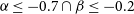
 $\alpha \leq -0.7 \cap \beta \leq -0.2$
. The first part of this expression is almost identical to the spectral steepness criterion used in D20 (
$\alpha \leq -0.7 \cap \beta \leq -0.2$
. The first part of this expression is almost identical to the spectral steepness criterion used in D20 (
 $\alpha < -0.7$
), while the second part was relaxed from
$\alpha < -0.7$
), while the second part was relaxed from
 $-1.0 < \beta < -0.4$
in the pilot project to a wider range, given the potential trajectories of the tracks mentioned above. The total number of sources that remained after this step was 1187.
$-1.0 < \beta < -0.4$
in the pilot project to a wider range, given the potential trajectories of the tracks mentioned above. The total number of sources that remained after this step was 1187.

Figure 1. The
 $\alpha$
–
$\alpha$
–
 $\beta$
parameter space for all isolated and compact GLEAM sources in the VIKING survey area that have curved low-frequency radio spectra with
$\beta$
parameter space for all isolated and compact GLEAM sources in the VIKING survey area that have curved low-frequency radio spectra with
 $S_{0} \geq 40$
mJy (see Section 2.2.2). Error bars on individual data points are not shown for the sake of clarity; however, in the bottom-right corner of the panel, we indicate the median uncertainties in
$S_{0} \geq 40$
mJy (see Section 2.2.2). Error bars on individual data points are not shown for the sake of clarity; however, in the bottom-right corner of the panel, we indicate the median uncertainties in
 $\alpha$
(
$\alpha$
(
 $\pm 0.08$
) and
$\pm 0.08$
) and
 $\beta$
(
$\beta$
(
 $\pm 0.55$
) for the sources in our sample. The paucity of sources near
$\pm 0.55$
) for the sources in our sample. The paucity of sources near
 $\beta=0$
is due to our
$\beta=0$
is due to our
 $\lvert\beta\rvert > \sigma_{\beta}$
selection criterion. HzRG candidates were mostly selected in the region of the plot delineated by the blue solid lines (
$\lvert\beta\rvert > \sigma_{\beta}$
selection criterion. HzRG candidates were mostly selected in the region of the plot delineated by the blue solid lines (
 $\alpha \leq -0.7 \cap \beta \leq -0.2$
). The seven sources that do not fully meet our selection criteria are marked (see discussion in Section 2.3). We do not show the full range of
$\alpha \leq -0.7 \cap \beta \leq -0.2$
). The seven sources that do not fully meet our selection criteria are marked (see discussion in Section 2.3). We do not show the full range of
 $\alpha$
and
$\alpha$
and
 $\beta$
values in the plot; indeed, extreme values often correspond to much poorer fits. One source in our sample, J1141
$\beta$
values in the plot; indeed, extreme values often correspond to much poorer fits. One source in our sample, J1141
 $-$
0158, is not visible in the figure as it has a very large curvature term (
$-$
0158, is not visible in the figure as it has a very large curvature term (
 $\beta = -6.5 \pm 2.7$
); in this case, the fit is likely significantly affected by the S/N in the lower part of the GLEAM band (see Figure 2). J0856
$\beta = -6.5 \pm 2.7$
); in this case, the fit is likely significantly affected by the S/N in the lower part of the GLEAM band (see Figure 2). J0856
 $+$
0223 and J0917
$+$
0223 and J0917
 $-$
0012 from the pilot study, also in our larger sample, are marked separately. Furthermore, we show the HzRGs J0924
$-$
0012 from the pilot study, also in our larger sample, are marked separately. Furthermore, we show the HzRGs J0924
 $-$
2201 (
$-$
2201 (
 $\alpha = -0.26 \pm 0.04$
;
$\alpha = -0.26 \pm 0.04$
;
 $\beta = -1.42 \pm 0.27$
) and J1530
$\beta = -1.42 \pm 0.27$
) and J1530
 $+$
1049 (
$+$
1049 (
 $\alpha = -1.31 \pm 0.28$
;
$\alpha = -1.31 \pm 0.28$
;
 $\beta = -4.8 \pm 2.2$
), both of which are detected in GLEAM in other parts of the sky not covered by VIKING. We can see that J0924
$\beta = -4.8 \pm 2.2$
), both of which are detected in GLEAM in other parts of the sky not covered by VIKING. We can see that J0924
 $-$
2201 would be missed by our selection criteria; this is because the source turns over in the middle of the GLEAM band (Figure 11 in Callingham et al. Reference Callingham2017; also see Section 6.2 and Figure 3 in this paper). J1530
$-$
2201 would be missed by our selection criteria; this is because the source turns over in the middle of the GLEAM band (Figure 11 in Callingham et al. Reference Callingham2017; also see Section 6.2 and Figure 3 in this paper). J1530
 $+$
1049 has a similar USS spectral index in the GLEAM band compared with its spectrum between TGSS and NVSS/FIRST (
$+$
1049 has a similar USS spectral index in the GLEAM band compared with its spectrum between TGSS and NVSS/FIRST (
 $\alpha^{1400}_{147.5} = -1.4 \pm 0.1$
; Saxena et al. Reference Saxena2018a,b), and
$\alpha^{1400}_{147.5} = -1.4 \pm 0.1$
; Saxena et al. Reference Saxena2018a,b), and
 $\lvert\beta\rvert$
, while large, also has a large uncertainty due to low S/N measurements at 92, 204, and 212 MHz. We analyse the broadband spectrum of J1530
$\lvert\beta\rvert$
, while large, also has a large uncertainty due to low S/N measurements at 92, 204, and 212 MHz. We analyse the broadband spectrum of J1530
 $+$
1049 in Section 6.2 and Figure 3. Lastly, we plot five tracks corresponding to the predicted observed-frame values of
$+$
1049 in Section 6.2 and Figure 3. Lastly, we plot five tracks corresponding to the predicted observed-frame values of
 $\alpha$
and
$\alpha$
and
 $\beta$
of a model source at a given redshift with particular rest-frame spectral indices and break frequencies. Along each track, redshift increases from right to left, and the star markers indicate
$\beta$
of a model source at a given redshift with particular rest-frame spectral indices and break frequencies. Along each track, redshift increases from right to left, and the star markers indicate
 $z=$
2, 4, 6 and 8. The tracks shown are not an exhaustive range of possibilities, but instead illustrate how the track trajectories can change depending on the underlying rest-frame spectrum of the source. The track model parameters correspond to the smoothly varying double- and triple-power-law fits that we use in this paper to model the broadband spectra of our targets (Equations (5) and (6)). Tracks 1, 2, 3, 4 and 5 move into our selection region at redshifts of 9.3 (not shown in the panel), 4.5, 2.7, 3.4 and 6.0, respectively. The track trajectories would continue to the upper left if the redshift is increased. If the (lower) rest-frame break frequency is below/above 500 MHz, then a particular track trajectory is still the same as plotted, but the position corresponding to a given redshift is further along the track to the left/right.
$z=$
2, 4, 6 and 8. The tracks shown are not an exhaustive range of possibilities, but instead illustrate how the track trajectories can change depending on the underlying rest-frame spectrum of the source. The track model parameters correspond to the smoothly varying double- and triple-power-law fits that we use in this paper to model the broadband spectra of our targets (Equations (5) and (6)). Tracks 1, 2, 3, 4 and 5 move into our selection region at redshifts of 9.3 (not shown in the panel), 4.5, 2.7, 3.4 and 6.0, respectively. The track trajectories would continue to the upper left if the redshift is increased. If the (lower) rest-frame break frequency is below/above 500 MHz, then a particular track trajectory is still the same as plotted, but the position corresponding to a given redshift is further along the track to the left/right.
Although we applied a number of selection criteria above to restrict the list of sources to those that are compact and isolated, source blending remains a potential issue that must be considered carefully given the relatively low angular resolution of the GLEAM data. This is particularly relevant regarding the reliability of the
 $\alpha$
and
$\alpha$
and
 $\beta$
measurements. We discuss this potential issue further in Section 5.4.3.
$\beta$
measurements. We discuss this potential issue further in Section 5.4.3.
2.2.3. Further selection criteria
To further reduce the fraction of low-redshift interlopers in our sample, step 8 in Table 1 was to remove those sources with mid-infrared detections in data from the Widefield Infrared Survey Explorer (WISE; Wright et al. Reference Wright2010), in particular the AllWISE (Cutri et al. Reference Cutri2014) data release. AllWISE is 95% complete to limiting magnitudes of 19.8, 19.0, 16.7, and 14.3 in the W1 (
 $3.37\, \unicode{x03BC} \mathrm{m}$
), W2 (
$3.37\, \unicode{x03BC} \mathrm{m}$
), W2 (
 $4.62 \,\unicode{x03BC} \mathrm{m}$
), W3 (
$4.62 \,\unicode{x03BC} \mathrm{m}$
), W3 (
 $12.1 \,\unicode{x03BC} \mathrm{m}$
) and W4 (
$12.1 \,\unicode{x03BC} \mathrm{m}$
) and W4 (
 $22.2 \,\unicode{x03BC} \mathrm{m}$
) bands, respectively. W1 and W2 are sufficiently comparable in depth to the
$22.2 \,\unicode{x03BC} \mathrm{m}$
) bands, respectively. W1 and W2 are sufficiently comparable in depth to the
 $K_{\rm s}$
-band visual selection that we describe below, and therefore step 8 increased the efficiency of our selection procedure (also see e.g. Sadler et al. Reference Sadler, Chhetri, Morgan, Mahony, Jarrett and Tingay2019). We searched for mid-infrared counterparts within
$K_{\rm s}$
-band visual selection that we describe below, and therefore step 8 increased the efficiency of our selection procedure (also see e.g. Sadler et al. Reference Sadler, Chhetri, Morgan, Mahony, Jarrett and Tingay2019). We searched for mid-infrared counterparts within
 $2^{\prime\prime}$
from the radio position in FIRST for EQU sources and TGSS for SGP sources; following e.g. Condon et al. (Reference Condon, Cotton, Greisen, Yin, Perley, Taylor and Broderick1998), to first order we would expect about 20 AllWISE–radio matches by chance for 1187 targets given the areal density of AllWISE sources.
$2^{\prime\prime}$
from the radio position in FIRST for EQU sources and TGSS for SGP sources; following e.g. Condon et al. (Reference Condon, Cotton, Greisen, Yin, Perley, Taylor and Broderick1998), to first order we would expect about 20 AllWISE–radio matches by chance for 1187 targets given the areal density of AllWISE sources.
We were then left with a reasonable number of sources, 753 in total, that could potentially be examined in more detail, particularly visual inspection of multi-wavelength data (step 9 in Table 1). An important caveat for step 9, however, is that while our sample selection technique is designed to be efficient, it is not complete. In particular, there were considerations regarding follow-up observing campaigns, for example ensuring an adequate typical signal-to-noise ratio (S/N) of the ATCA data that we present in Section 4. In practice, we visually inspected about half of the 753 sources.
For the visual inspection, the primary check was to overlay radio contours on the VIKING
 $K_{\rm s}$
-band images. The goal was to identify those sources that were sufficiently compact in the radio and not detected in VIKING at the
$K_{\rm s}$
-band images. The goal was to identify those sources that were sufficiently compact in the radio and not detected in VIKING at the
 $5\sigma$
level (the latter confirmed from analysis of the reprocessed images and not from the latest VIKING catalogue available in the literature, i.e. Edge et al. Reference Edge, Sutherland and Viking Team2016); these sources were then deemed to be the best HzRG candidates for further follow-up and analysis. We used the radio data from TGSS, NVSS and FIRST that had been considered in the previous steps as well as higher-resolution radio data that became available during the course of our analysis: 887.5-MHz images from the Rapid Australian Square Kilometre Array Pathfinder (ASKAP; Johnston et al. Reference Johnston2007; Hotan et al. Reference Hotan2021) Continuum Survey (RACS; McConnell et al. Reference McConnell2020; Hale et al. Reference Hale2021) and 3-GHz ‘quick-look’ images from the first epoch of the VLA Sky Survey (VLASS; Lacy et al. Reference Lacy2020). Furthermore, for the
$5\sigma$
level (the latter confirmed from analysis of the reprocessed images and not from the latest VIKING catalogue available in the literature, i.e. Edge et al. Reference Edge, Sutherland and Viking Team2016); these sources were then deemed to be the best HzRG candidates for further follow-up and analysis. We used the radio data from TGSS, NVSS and FIRST that had been considered in the previous steps as well as higher-resolution radio data that became available during the course of our analysis: 887.5-MHz images from the Rapid Australian Square Kilometre Array Pathfinder (ASKAP; Johnston et al. Reference Johnston2007; Hotan et al. Reference Hotan2021) Continuum Survey (RACS; McConnell et al. Reference McConnell2020; Hale et al. Reference Hale2021) and 3-GHz ‘quick-look’ images from the first epoch of the VLA Sky Survey (VLASS; Lacy et al. Reference Lacy2020). Furthermore, for the
 $K_{\rm s}$
-band non-detections, we also inspected the corresponding reprocessed J-band (
$K_{\rm s}$
-band non-detections, we also inspected the corresponding reprocessed J-band (
 $1.25 \,\unicode{x03BC} \mathrm{m}$
) and H-band (
$1.25 \,\unicode{x03BC} \mathrm{m}$
) and H-band (
 $1.64 \,\unicode{x03BC} \mathrm{m}$
) VIKING images from the GAMA collaboration (target
$1.64 \,\unicode{x03BC} \mathrm{m}$
) VIKING images from the GAMA collaboration (target
 $5\sigma$
magnitude limits of 22.1 and 21.5, respectively) to check that each host galaxy was not detected in these bands either at the
$5\sigma$
magnitude limits of 22.1 and 21.5, respectively) to check that each host galaxy was not detected in these bands either at the
 $5\sigma$
level. As above for the AllWISE–radio cross-correlation, to first order we would expect
$5\sigma$
level. As above for the AllWISE–radio cross-correlation, to first order we would expect
 $\sim$
10 sources to have been filtered out due to a VIKING–radio association by chance given the areal density of VIKING sources.
$\sim$
10 sources to have been filtered out due to a VIKING–radio association by chance given the areal density of VIKING sources.
After confirming the radio morphology in each case, we removed all sources with a largest angular sizeFootnote c (LAS)
 $>5^{\prime\prime}$
in FIRST and/or VLASS (e.g. projected linear size
$>5^{\prime\prime}$
in FIRST and/or VLASS (e.g. projected linear size
 ${<}32.1$
kpc at
${<}32.1$
kpc at
 $z > 5$
). If there was sufficient uncertainty regarding the angular extent of the radio emission, particularly if a potential HzRG candidate was instead possibly a single component of a larger radio source, we erred on the side of caution and removed the candidate in question from the sample. Our LAS cutoff is a somewhat arbitrary choice, but such a cutoff can improve the efficiency of an HzRG search (e.g. Ker et al. Reference Ker, Best, Rigby, Röttgering and Gendre2012). From the ALMA data presented in D20, LAS
$z > 5$
). If there was sufficient uncertainty regarding the angular extent of the radio emission, particularly if a potential HzRG candidate was instead possibly a single component of a larger radio source, we erred on the side of caution and removed the candidate in question from the sample. Our LAS cutoff is a somewhat arbitrary choice, but such a cutoff can improve the efficiency of an HzRG search (e.g. Ker et al. Reference Ker, Best, Rigby, Röttgering and Gendre2012). From the ALMA data presented in D20, LAS
 $= 4 .\!^{\prime\prime} 9$
for J0856
$= 4 .\!^{\prime\prime} 9$
for J0856
 $+$
0223, which is the largest of the three currently known radio galaxies at
$+$
0223, which is the largest of the three currently known radio galaxies at
 $z > 5$
. Assuming the modelling of Saxena et al. (Reference Saxena, Röttgering and Rigby2017), a selection criterion of LAS
$z > 5$
. Assuming the modelling of Saxena et al. (Reference Saxena, Röttgering and Rigby2017), a selection criterion of LAS
 ${\leq}5^{\prime\prime}$
would be sensitive to radio galaxies at redshifts beyond that of J1530
${\leq}5^{\prime\prime}$
would be sensitive to radio galaxies at redshifts beyond that of J1530
 $+$
1049 at
$+$
1049 at
 $z=5.72$
(see Figure 15 in Saxena et al. Reference Saxena2019). One caveat is that we would then filter out larger HzRGs that may exist in the early Universe if the jets grow on shorter timescales than predicted in the Saxena et al. (Reference Saxena, Röttgering and Rigby2017) framework, as is suggested from modelling based on different assumptions (Turner et al. Reference Turner, Rogers, Shabala and Krause2018; Turner et al. in preparation).
$z=5.72$
(see Figure 15 in Saxena et al. Reference Saxena2019). One caveat is that we would then filter out larger HzRGs that may exist in the early Universe if the jets grow on shorter timescales than predicted in the Saxena et al. (Reference Saxena, Röttgering and Rigby2017) framework, as is suggested from modelling based on different assumptions (Turner et al. Reference Turner, Rogers, Shabala and Krause2018; Turner et al. in preparation).
Apart from searching for VIKING non-detections, we also inspected images, where available, from the second data release of the Hyper Suprime-Cam (Miyazaki et al. Reference Miyazaki2018) Subaru Strategic Program (Aihara et al. Reference Aihara2018, Reference Aihara2019), removing any sources from our candidate list with deep Y-band (
 $0.98\,\unicode{x03BC}$
m) detections (
$0.98\,\unicode{x03BC}$
m) detections (
 $5\sigma$
magnitude limit
$5\sigma$
magnitude limit
 $= 24.2$
in a
$= 24.2$
in a
 $2^{\prime\prime}$
-diameter aperture). We also searched the ATNF pulsar database (Manchester et al. Reference Manchester, Hobbs, Teoh and Hobbs2005)Footnote d, finding no known pulsars at the positions of the HzRG candidates presented in this paper.
$2^{\prime\prime}$
-diameter aperture). We also searched the ATNF pulsar database (Manchester et al. Reference Manchester, Hobbs, Teoh and Hobbs2005)Footnote d, finding no known pulsars at the positions of the HzRG candidates presented in this paper.
Lastly, when we had nearly finalised our sample, some data became available from SHARKS, which is a deep survey of
 ${\sim} 300\ \mathrm{deg}^2$
conducted with the VISTA telescope, covering several H-ATLAS fields, with a target
${\sim} 300\ \mathrm{deg}^2$
conducted with the VISTA telescope, covering several H-ATLAS fields, with a target
 $5\sigma$
magnitude limit of
$5\sigma$
magnitude limit of
 $K_{\rm s} \sim 22.7$
. Details on the survey strategy and data reduction were presented in Dannerbauer et al. (Reference Dannerbauer, Carnero, Cross and Gutierrez2022). The data that we used were from observations conducted between 2017 March and 2019 January. We removed sources with SHARKS detections and noted those sources with SHARKS non-detections, which remained in the sample (discussed further in Section 3).
$K_{\rm s} \sim 22.7$
. Details on the survey strategy and data reduction were presented in Dannerbauer et al. (Reference Dannerbauer, Carnero, Cross and Gutierrez2022). The data that we used were from observations conducted between 2017 March and 2019 January. We removed sources with SHARKS detections and noted those sources with SHARKS non-detections, which remained in the sample (discussed further in Section 3).
2.3. The GLEAM–VIKING HzRG candidate sample
After applying the criteria described in Section 2.2.3, we were left with a sample of 53 sources within the VIKING survey region (step 10 in Table 1). The sample comprises 51 new HzRG candidates and both J0856
 $+$
0223 and J0917
$+$
0223 and J0917
 $-$
0012 from our pilot study (Section 1), which satisfy the refined selection criteria used in this paper.Footnote e Note that the sample includes six sources that do not fully meet the
$-$
0012 from our pilot study (Section 1), which satisfy the refined selection criteria used in this paper.Footnote e Note that the sample includes six sources that do not fully meet the
 $\alpha$
and
$\alpha$
and
 $\beta$
selection criteria: J0034
$\beta$
selection criteria: J0034
 $-$
3112, J0053
$-$
3112, J0053
 $-$
3256, J0129
$-$
3256, J0129
 $-$
3109, J1037
$-$
3109, J1037
 $-$
0325, J1246
$-$
0325, J1246
 $-$
0017 and J2311
$-$
0017 and J2311
 $-$
3359. For all of these sources bar one, this is because (i) they marginally fall outside of our selection region in
$-$
3359. For all of these sources bar one, this is because (i) they marginally fall outside of our selection region in
 $\alpha$
–
$\alpha$
–
 $\beta$
parameter space (Figure 1), yet within the
$\beta$
parameter space (Figure 1), yet within the
 $1\sigma$
uncertainties they are consistent with the selection criteria, or (ii)
$1\sigma$
uncertainties they are consistent with the selection criteria, or (ii)
 $\lvert\beta\rvert$
is marginally smaller than
$\lvert\beta\rvert$
is marginally smaller than
 $\sigma_{\beta}$
. Our original approach for the
$\sigma_{\beta}$
. Our original approach for the
 $\alpha$
–
$\alpha$
–
 $\beta$
fitting had been to use Equation (1), and due to the propagation of the flux density uncertainties in
$\beta$
fitting had been to use Equation (1), and due to the propagation of the flux density uncertainties in
 $\log\!{(S_{\nu}})$
–
$\log\!{(S_{\nu}})$
–
 $\log\!{(\nu)}$
space, these sources initially fully satisfied our selection criteria and had been followed up with the ATCA (Section 4). The remaining source, J2311
$\log\!{(\nu)}$
space, these sources initially fully satisfied our selection criteria and had been followed up with the ATCA (Section 4). The remaining source, J2311
 $-$
3359 from the GAMA-23 field, was removed in step 2 in Table 1, as it is too faint to be detected in NVSS; moreover, it does not satisfy our
$-$
3359 from the GAMA-23 field, was removed in step 2 in Table 1, as it is too faint to be detected in NVSS; moreover, it does not satisfy our
 $\lvert\beta\rvert > \sigma_{\beta}$
criterion, and ASKAP early science data suggests an LAS of
$\lvert\beta\rvert > \sigma_{\beta}$
criterion, and ASKAP early science data suggests an LAS of
 $5.\!^{\prime\prime}6$
(see Section 5.5). J2311
$5.\!^{\prime\prime}6$
(see Section 5.5). J2311
 $-$
3359 was identified as an HzRG candidate of particular interest given its USS nature (
$-$
3359 was identified as an HzRG candidate of particular interest given its USS nature (
 $\alpha = -1.58 \pm 0.19$
in GLEAM) and followed up with the ATCA before the selection criteria for this project were fully defined.
$\alpha = -1.58 \pm 0.19$
in GLEAM) and followed up with the ATCA before the selection criteria for this project were fully defined.
In addition to these six sources, our sample includes the source J1335
 $+$
0112. This source meets all of our selection criteria except that it has an AllWISE identification (which we discuss later in Section 5.5). Unfortunately, this source was followed up with the ATCA before our
$+$
0112. This source meets all of our selection criteria except that it has an AllWISE identification (which we discuss later in Section 5.5). Unfortunately, this source was followed up with the ATCA before our
 $2^{\prime\prime}$
AllWISE criteria was introduced (it had been
$2^{\prime\prime}$
AllWISE criteria was introduced (it had been
 $1^{\prime\prime}$
). As we outline in Section 5.5, J1335
$1^{\prime\prime}$
). As we outline in Section 5.5, J1335
 $+$
0112 may still be a high-redshift target, and therefore we decided that there was sufficient scientific interest to include the source in our sample.
$+$
0112 may still be a high-redshift target, and therefore we decided that there was sufficient scientific interest to include the source in our sample.
The sample is presented in Table 2, including the
 $\alpha$
and
$\alpha$
and
 $\beta$
values for each source and the fitted 151-MHz GLEAM flux density. The fitted 151-MHz flux densities span the range 47.6–2439 mJy, with a median of 260.6 mJy. We have marked the locations of the sources in our sample in the
$\beta$
values for each source and the fitted 151-MHz GLEAM flux density. The fitted 151-MHz flux densities span the range 47.6–2439 mJy, with a median of 260.6 mJy. We have marked the locations of the sources in our sample in the
 $\alpha$
–
$\alpha$
–
 $\beta$
parameter space in Figure 1. The median spectral index of the sample at 151 MHz is
$\beta$
parameter space in Figure 1. The median spectral index of the sample at 151 MHz is
 $-0.96$
, and only three sources would be traditionally classified as USS with
$-0.96$
, and only three sources would be traditionally classified as USS with
 $\alpha \leq -1.3$
: J0007
$\alpha \leq -1.3$
: J0007
 $-$
3040, J2311
$-$
3040, J2311
 $-$
3359 (discussed above) and J2314
$-$
3359 (discussed above) and J2314
 $-$
3517.
$-$
3517.
3. Near-infrared
 $\boldsymbol{K}_{\textbf{s}}$
-band data
$\boldsymbol{K}_{\textbf{s}}$
-band data

In this section, we summarise the
 $K_{\rm s}$
-band data for our sample. All sources are not detected in VIKING at the
$K_{\rm s}$
-band data for our sample. All sources are not detected in VIKING at the
 $5\sigma$
level, but deeper limits or detections are available in some cases.
$5\sigma$
level, but deeper limits or detections are available in some cases.
Firstly, as presented in D20, J0856
 $+$
0223 and J0917
$+$
0223 and J0917
 $-$
0012 were observed with VLT/HAWK-I. The host galaxy was detected in both cases; the magnitudes are
$-$
0012 were observed with VLT/HAWK-I. The host galaxy was detected in both cases; the magnitudes are
 $23.2 \pm 0.1$
(J0856
$23.2 \pm 0.1$
(J0856
 $+$
0223) and
$+$
0223) and
 $23.01 \pm 0.04$
(J0917
$23.01 \pm 0.04$
(J0917
 $-$
0012; see the most recent analysis in Seymour et al. Reference Seymour2022).
$-$
0012; see the most recent analysis in Seymour et al. Reference Seymour2022).
J0133
 $-$
3056 and J0842
$-$
3056 and J0842
 $-$
0157 were also observed with HAWK-I as part of the ESO service-mode ‘filler’ programme 0104.A-0599(A). The eight targets for which data were obtained were a combination of USS sources and those selected from an earlier version of the curved-spectrum technique described in Section 2.2. For both J0133
$-$
0157 were also observed with HAWK-I as part of the ESO service-mode ‘filler’ programme 0104.A-0599(A). The eight targets for which data were obtained were a combination of USS sources and those selected from an earlier version of the curved-spectrum technique described in Section 2.2. For both J0133
 $-$
3056 and J0842
$-$
3056 and J0842
 $-$
0157, the exposure time was 35 min using a standard jitter pattern. We ran the source-finding code sextractor (Bertin & Arnouts Reference Bertin and Arnouts1996) on the pipeline-reduced images. We measured magnitudes within an aperture of diameter
$-$
0157, the exposure time was 35 min using a standard jitter pattern. We ran the source-finding code sextractor (Bertin & Arnouts Reference Bertin and Arnouts1996) on the pipeline-reduced images. We measured magnitudes within an aperture of diameter
 $2^{\prime\prime}$
(one of several standard choices for HzRG
$2^{\prime\prime}$
(one of several standard choices for HzRG
 $K_{\rm s}$
-band measurements in the literature; e.g. De Breuck et al. Reference De Breuck, van Breugel, Stanford, Röttgering, Miley and Stern2002) and applied an aperture correction derived from a curve of growth of
$K_{\rm s}$
-band measurements in the literature; e.g. De Breuck et al. Reference De Breuck, van Breugel, Stanford, Röttgering, Miley and Stern2002) and applied an aperture correction derived from a curve of growth of
 $-$
0.16 mag. To confirm the photometric scale, we cross-matched the sextractor source catalogues from the pipeline-produced images with the Two-Micron All Sky Survey (2MASS; Skrutskie et al. Reference Skrutskie2006), using a maximum search radius of
$-$
0.16 mag. To confirm the photometric scale, we cross-matched the sextractor source catalogues from the pipeline-produced images with the Two-Micron All Sky Survey (2MASS; Skrutskie et al. Reference Skrutskie2006), using a maximum search radius of
 $1.\!^{\prime\prime}5$
. In both cases, the difference was
$1.\!^{\prime\prime}5$
. In both cases, the difference was
 ${\leq}0.1$
mag; therefore, an associated correction was not applied. The final
${\leq}0.1$
mag; therefore, an associated correction was not applied. The final
 $K_{\rm s}$
-band aperture magnitudes, converted from Vega to AB, are
$K_{\rm s}$
-band aperture magnitudes, converted from Vega to AB, are
 $22.96 \pm 0.12$
(J0842
$22.96 \pm 0.12$
(J0842
 $-$
0157) and
$-$
0157) and
 $22.23 \pm 0.08$
(J0133
$22.23 \pm 0.08$
(J0133
 $-$
3056); further discussion can be found in Section 5.5. The uncertainties are the combination of the measurement uncertainty and a 10% calibration uncertainty.
$-$
3056); further discussion can be found in Section 5.5. The uncertainties are the combination of the measurement uncertainty and a 10% calibration uncertainty.
Three of the sources, J0007
 $-$
3040, J0008
$-$
3040, J0008
 $-$
3007 and J2340
$-$
3007 and J2340
 $-$
3230, are not detected in SHARKS. Using the information available from the SHARKS data products (Dannerbauer et al. Reference Dannerbauer, Carnero, Cross and Gutierrez2022), the
$-$
3230, are not detected in SHARKS. Using the information available from the SHARKS data products (Dannerbauer et al. Reference Dannerbauer, Carnero, Cross and Gutierrez2022), the
 $5\sigma$
magnitude lower limits are 23.1 (J0007
$5\sigma$
magnitude lower limits are 23.1 (J0007
 $-$
3040 and J0008
$-$
3040 and J0008
 $-$
3007) and 22.9 (J2340
$-$
3007) and 22.9 (J2340
 $-$
3230); the respective observations were deeper than the target
$-$
3230); the respective observations were deeper than the target
 $5\sigma$
limit of 22.7.
$5\sigma$
limit of 22.7.
Table 2. Radio properties of our sample listed in order of right ascension. We list whether the source is in the equatorial VIKING strip (i.e. covered by GLEAM Exgal) or the south Galactic pole strip (i.e. covered by GLEAM SGP). Here we report the fitted 151-MHz GLEAM flux density from Section 2.2.2 only; the full set of catalogued GLEAM flux densities can be found in Hurley-Walker et al. (Reference Hurley-Walker2017) and Franzen et al. (Reference Franzen, Hurley-Walker, White, Hancock, Seymour, Kapińska, Staveley-Smith and Wayth2021). TGSS flux densities at 147.5 MHz are from a rescaled version of this catalogue (Hurley-Walker Reference Hurley-Walker2017). FIRST and NVSS 1400-MHz flux densities are reported (denoted by the subscripts F and N, respectively). The SUMSS and NVSS flux density upper limits for J2311
 $-$
3359 are at the
$-$
3359 are at the
 $3\sigma$
level. Various table entries with a horizontal ellipsis (
$3\sigma$
level. Various table entries with a horizontal ellipsis (
 $\cdots$
) indicate that observations are not available at a particular frequency because either the source is not located within the sky coverage of the survey (SUMSS and FIRST) or observations were not taken (ATCA). For the SGP sources, we report the ATCA and VLASS LAS values (in this order); similarly, for the equatorial sources, we report the FIRST and VLASS LAS values (again in this order). For the ATCA LAS measurements, where we have two observing frequencies, we took into account both angular resolution and S/N so as to choose the best LAS measurement from a given 5.5- and 9-GHz pair; this was generally the value at 9 GHz for sufficiently high S/N. FIRST and VLASS LAS measurements are from Helfand et al. (Reference Helfand, White and Becker2015) and Gordon et al. (Reference Gordon2020), respectively. LAS upper limits were calculated using a
$\cdots$
) indicate that observations are not available at a particular frequency because either the source is not located within the sky coverage of the survey (SUMSS and FIRST) or observations were not taken (ATCA). For the SGP sources, we report the ATCA and VLASS LAS values (in this order); similarly, for the equatorial sources, we report the FIRST and VLASS LAS values (again in this order). For the ATCA LAS measurements, where we have two observing frequencies, we took into account both angular resolution and S/N so as to choose the best LAS measurement from a given 5.5- and 9-GHz pair; this was generally the value at 9 GHz for sufficiently high S/N. FIRST and VLASS LAS measurements are from Helfand et al. (Reference Helfand, White and Becker2015) and Gordon et al. (Reference Gordon2020), respectively. LAS upper limits were calculated using a
 $5\sigma$
upper bound on the deconvolved major axis FWHM (from the pybdsf output, or, for the FIRST LAS upper limit for J1246
$5\sigma$
upper bound on the deconvolved major axis FWHM (from the pybdsf output, or, for the FIRST LAS upper limit for J1246
 $-$
0017, following e.g. Fomalont Reference Fomalont, Taylor, Carilli and Perley1999), except for J2311
$-$
0017, following e.g. Fomalont Reference Fomalont, Taylor, Carilli and Perley1999), except for J2311
 $-$
3559 where the upper limit is taken as the 9-GHz synthesised beam major axis FWHM. See Sections 2, 4, and 5 for further details.
$-$
3559 where the upper limit is taken as the 9-GHz synthesised beam major axis FWHM. See Sections 2, 4, and 5 for further details.

Notes.
 ${}^{\rm \dagger}$
These sources do not satisfy all of our selection criteria (see Section 2.3).
${}^{\rm \dagger}$
These sources do not satisfy all of our selection criteria (see Section 2.3).
 ${}^{\rm a}$
Uncertainties are not given in the catalogue, but see Becker et al. (Reference Becker, White and Helfand1995), Helfand et al. (Reference Helfand, White and Becker2015) and https://sundog.stsci.edu/first/catalogs/readme.html for further details.
${}^{\rm a}$
Uncertainties are not given in the catalogue, but see Becker et al. (Reference Becker, White and Helfand1995), Helfand et al. (Reference Helfand, White and Becker2015) and https://sundog.stsci.edu/first/catalogs/readme.html for further details.
 ${}^{\rm b}$
Estimated from visual inspection and subsequent analysis of the image of this source.
${}^{\rm b}$
Estimated from visual inspection and subsequent analysis of the image of this source.
 ${}^{\rm c}$
One LAS measurement only for J0133
${}^{\rm c}$
One LAS measurement only for J0133
 $-$
3056 (VLASS; no ATCA observations taken), J1521
$-$
3056 (VLASS; no ATCA observations taken), J1521
 $-$
0104 (FIRST; insufficient S/N in VLASS) and J2311
$-$
0104 (FIRST; insufficient S/N in VLASS) and J2311
 $-$
3359 (ATCA; insufficient S/N in VLASS). The LAS for J2311
$-$
3359 (ATCA; insufficient S/N in VLASS). The LAS for J2311
 $-$
3359 may be larger than our
$-$
3359 may be larger than our
 $5^{\prime\prime}$
cutoff (see Section 5.5).
$5^{\prime\prime}$
cutoff (see Section 5.5).
 ${}^{\rm d}$
Source is from the pilot study; see Section 1 and D20 for further details. Note that the 5.5- and 9-GHz flux densities are from the ATCA observations presented in D20.
${}^{\rm d}$
Source is from the pilot study; see Section 1 and D20 for further details. Note that the 5.5- and 9-GHz flux densities are from the ATCA observations presented in D20.
 ${}^{\rm e}$
8.8-GHz flux densities; other flux density values in this column without a footnote are 9-GHz values.
${}^{\rm e}$
8.8-GHz flux densities; other flux density values in this column without a footnote are 9-GHz values.
For the remaining 46 sources in the sample with VIKING
 $K_{\rm s}$
-band non-detections, we calculated the
$K_{\rm s}$
-band non-detections, we calculated the
 $5\sigma$
magnitude lower limits as follows:
$5\sigma$
magnitude lower limits as follows:
 \begin{equation}K_{\rm{s,\,5\sigma}} = m_{\rm ZP} - 2.5\log\!(5\sigma_{\rm ADU} \times 1.13309 \times \theta^2).\end{equation}
In Equation (3),
 $\sigma_{\rm ADU}$
is the root-mean-square (RMS) standard deviation in the vicinity of the radio position in analogue-to-digital units (ADU),
$\sigma_{\rm ADU}$
is the root-mean-square (RMS) standard deviation in the vicinity of the radio position in analogue-to-digital units (ADU),
 $m_{\rm ZP}$
is the zero-point magnitude (30.0),
$m_{\rm ZP}$
is the zero-point magnitude (30.0),
 $\theta$
is the seeing disc FWHM in pixels (median seeing
$\theta$
is the seeing disc FWHM in pixels (median seeing
 $0.\!^{\prime\prime} 83$
; pixel size
$0.\!^{\prime\prime} 83$
; pixel size
 $0.\!^{\prime\prime} 339$
), and the factor 1.13309 is from the standard formula for a two-dimensional Gaussian function. The
$0.\!^{\prime\prime} 339$
), and the factor 1.13309 is from the standard formula for a two-dimensional Gaussian function. The
 $5\sigma$
VIKING limits span the range 21.2–22.3, with a median of 21.7, i.e. deeper than the 5
$5\sigma$
VIKING limits span the range 21.2–22.3, with a median of 21.7, i.e. deeper than the 5
 $\sigma$
target limit of 21.2.
$\sigma$
target limit of 21.2.
The
 $K_{\rm s}$
-band images for the 51 new HzRG candidates are presented in Section 5 (Figure 2).
$K_{\rm s}$
-band images for the 51 new HzRG candidates are presented in Section 5 (Figure 2).

Figure 2. Overlay plots (left) and observed-frame broadband radio spectra (right) for all of the sources in our sample apart from J0856
 $+$
0223 and J0917
$+$
0223 and J0917
 $-$
0012 from the pilot study. The
$-$
0012 from the pilot study. The
 $K_{\rm s}$
-band image used in each overlay plot is listed. We plot FIRST (orange) and VLASS (magenta) contours for the EQU sources; similarly, we plot VLASS, ATCA 5.5-GHz (blue) and ATCA 9-GHz (red) contours for the SGP sources (note that J0133
$K_{\rm s}$
-band image used in each overlay plot is listed. We plot FIRST (orange) and VLASS (magenta) contours for the EQU sources; similarly, we plot VLASS, ATCA 5.5-GHz (blue) and ATCA 9-GHz (red) contours for the SGP sources (note that J0133
 $-$
3056 has VLASS data only). ATCA contours are not shown for the EQU sources given the poorer angular resolution compared to FIRST and VLASS. The contours are a geometric progression in
$-$
3056 has VLASS data only). ATCA contours are not shown for the EQU sources given the poorer angular resolution compared to FIRST and VLASS. The contours are a geometric progression in
 $\sqrt{2}$
, with the lowest contour usually at the
$\sqrt{2}$
, with the lowest contour usually at the
 $5\sigma$
level. A summary of the lowest contour levels used in each overlay plot can be found in Table 5. Radio synthesised beams are shown in each overlay plot with different hatching styles (FIRST: horizontal; VLASS: vertical; ATCA 5.5 GHz: forward slash; ATCA 9 GHz: backslash). For the broadband radio spectra, we plot the data presented in Tables 2 and 4, apart from the 151-MHz GLEAM fitted flux densities and the 1400-MHz FIRST flux densities in Table 2 (in the latter case we show the NVSS flux density measurements only). Additionally, we plot catalogued GLEAM flux densities (20 measurements per source) from Hurley-Walker et al. (Reference Hurley-Walker2017, EQU sources) and Franzen et al. (Reference Franzen, Hurley-Walker, White, Hancock, Seymour, Kapińska, Staveley-Smith and Wayth2021, SGP sources). In each panel, the GLEAM data points are shown as red circles and the remaining data points as black squares. In addition, the solid line represents the preferred model (either a single or double power law, indicated in each plot legend as SPL and DPL, respectively). In the panel showing the radio spectrum for J2311
$5\sigma$
level. A summary of the lowest contour levels used in each overlay plot can be found in Table 5. Radio synthesised beams are shown in each overlay plot with different hatching styles (FIRST: horizontal; VLASS: vertical; ATCA 5.5 GHz: forward slash; ATCA 9 GHz: backslash). For the broadband radio spectra, we plot the data presented in Tables 2 and 4, apart from the 151-MHz GLEAM fitted flux densities and the 1400-MHz FIRST flux densities in Table 2 (in the latter case we show the NVSS flux density measurements only). Additionally, we plot catalogued GLEAM flux densities (20 measurements per source) from Hurley-Walker et al. (Reference Hurley-Walker2017, EQU sources) and Franzen et al. (Reference Franzen, Hurley-Walker, White, Hancock, Seymour, Kapińska, Staveley-Smith and Wayth2021, SGP sources). In each panel, the GLEAM data points are shown as red circles and the remaining data points as black squares. In addition, the solid line represents the preferred model (either a single or double power law, indicated in each plot legend as SPL and DPL, respectively). In the panel showing the radio spectrum for J2311
 $-$
3359, triangles represent
$-$
3359, triangles represent
 $3\sigma$
flux density upper limits (Table 2), but we did not use these upper limits when modelling its radio spectrum. The 365-MHz data point for J1317
$3\sigma$
flux density upper limits (Table 2), but we did not use these upper limits when modelling its radio spectrum. The 365-MHz data point for J1317
 $+$
0339, a clear outlier, was also not used in the modelling. Error bars are
$+$
0339, a clear outlier, was also not used in the modelling. Error bars are
 $\pm1\sigma$
. In a few of the panels, the relative GLEAM flux density uncertainties at certain frequencies are larger than 100%, and therefore the full extent of the lower error bar cannot be shown on a log–log plot. See Section 5.4 for a description of the modelling and Table 7 for the fitted parameters from each preferred model.
$\pm1\sigma$
. In a few of the panels, the relative GLEAM flux density uncertainties at certain frequencies are larger than 100%, and therefore the full extent of the lower error bar cannot be shown on a log–log plot. See Section 5.4 for a description of the modelling and Table 7 for the fitted parameters from each preferred model.
4. ATCA data
To facilitate modelling of each radio spectrum and, where possible, to obtain further high-resolution radio data to help confirm the compact radio morphologies and
 $K_{\rm s}$
-band non-detections, we observed 49 of the 53 sources in our sample with the ATCA as part of projects CX437 and C3377. Of the remaining four sources, J0856
$K_{\rm s}$
-band non-detections, we observed 49 of the 53 sources in our sample with the ATCA as part of projects CX437 and C3377. Of the remaining four sources, J0856
 $+$
0223 and J0917
$+$
0223 and J0917
 $-$
0012 were observed with the ATCA as part of the D20 pilot study. J0133
$-$
0012 were observed with the ATCA as part of the D20 pilot study. J0133
 $-$
3056 and J0842
$-$
3056 and J0842
 $-$
0157 were not observed as these sources were originally considered to be part of another closely related HzRG project (i.e. the
$-$
0157 were not observed as these sources were originally considered to be part of another closely related HzRG project (i.e. the
 $K_{\rm s}$
-band ‘filler’ targets discussed in Section 3), before being added to the sample presented in this paper. ATCA data are not available for these sources in the Australia Telescope Online Archive.Footnote f
$K_{\rm s}$
-band ‘filler’ targets discussed in Section 3), before being added to the sample presented in this paper. ATCA data are not available for these sources in the Australia Telescope Online Archive.Footnote f
4.1. Projects CX437 and C3377
An observing log for our ATCA observations is presented in Table 3. Observations were carried out simultaneously at 5.5 and 9 GHz using the Compact Array Broadband Backend (CABB; Wilson et al. Reference Wilson2011), with a nominal bandwidth of 2.048 GHz at each frequency comprising
 $2048 \times 1$
-MHz channels. We used a general observational strategy of target snapshots interleaved with scans of phase calibrators. When more than one target was observed, we ensured that the individual snapshots were sufficiently well spread in hour angle to give sufficient (u, v) coverage for imaging. The standard primary calibrator PKS B1934
$2048 \times 1$
-MHz channels. We used a general observational strategy of target snapshots interleaved with scans of phase calibrators. When more than one target was observed, we ensured that the individual snapshots were sufficiently well spread in hour angle to give sufficient (u, v) coverage for imaging. The standard primary calibrator PKS B1934
 $-$
638 was observed in each run, with the flux density scale reported in Reynolds (Reference Reynolds1994).
$-$
638 was observed in each run, with the flux density scale reported in Reynolds (Reference Reynolds1994).
Table 3. ATCA observing log for our 5.5- and 9-GHz observations. On 2020 December 2/3, the effective frequency of the upper band was 8.8 rather than 9 GHz. Noise levels are those measured near the target; for the C3377 data, we give the median noise levels at 5.5 and 8.8/9 GHz. Furthermore, for the C3377 data, the reported angular resolutions were determined by taking the separate medians of the major and minor axis FWHMs as well as the BPAs. PKS B1934
 $-$
638 was the primary calibrator in all of the observing runs. Further details on the ATCA observations can be found in Section 4.
$-$
638 was the primary calibrator in all of the observing runs. Further details on the ATCA observations can be found in Section 4.

In project CX437, we used available Director’s Discretionary Time to observe J2311
 $-$
3359. The array was in the 750C configuration. 20-min target scans were interleaved with 2-min phase calibrator observations. Note that these observations were set up differently to what we describe below for C3377; this was due to the fact that the expected very faint flux densities for J2311
$-$
3359. The array was in the 750C configuration. 20-min target scans were interleaved with 2-min phase calibrator observations. Note that these observations were set up differently to what we describe below for C3377; this was due to the fact that the expected very faint flux densities for J2311
 $-$
3359 at 5.5 and 9 GHz required a significantly longer on-source integration time to increase the likelihood of a detection.
$-$
3359 at 5.5 and 9 GHz required a significantly longer on-source integration time to increase the likelihood of a detection.
In project C3377, we observed the remaining 48 sources. Observations were carried out with the 6A array configuration for the SGP targets and with the hybrid H168 array configuration for the EQU sources. The H168 configuration was needed for the EQU sources to ensure adequate (u, v) coverage. The individual target scans were mostly 3 min in duration, although with some variations. Phase calibrators were observed every
 $\sim$
10–25 min and the scans were either 1 or 1.5 min in duration.
$\sim$
10–25 min and the scans were either 1 or 1.5 min in duration.
4.2. Data reduction and imaging
The data were reduced and imaged using standard procedures in miriad (Sault, Teuben, & Wright Reference Sault, Teuben, Wright, Shaw, Payne and Hayes1995). Radio-frequency interference (RFI) was particularly problematic in our observing run on 2020 December 2/3; hence, a significant amount of primary calibrator data in the upper part of the 9-GHz band had to be flagged. To make the subsequent flux density calibration of the phase calibrator and target data as straightforward as possible, we also flagged the corresponding channels in these data, resulting in a nominal sensitivity penalty of about 10–15% and a shift in the effective frequency from 9 to 8.8 GHz.
When the S/N was sufficient, we used several iterations of imaging and phase-only self-calibration, the latter based on the clean component models. We used multifrequency deconvolution (Sault & Wieringa Reference Sault and Wieringa1994) and the robust weighting parameter (Briggs Reference Briggs1995) was set to 0.5. Note that we did not include baselines to antenna 6 in the imaging and self-calibration step for the data from project CX437 as well as the H168 observations from C3377. This was to remove the large gap in the (u, v) coverage, with a nominal sensitivity penalty of about 20% and poorer angular resolution. However, high-resolution data were already available from FIRST and VLASS for these targets. The maximum antenna spacings for our ATCA data sets were then 192, 750 and 5939 m for the H168, 750C and 6A observations, respectively. A primary beam correction was applied to all cleaned maps, although this did not make a significant difference to the integrated flux densities as all of our targets were at or very close to the pointing centre. Angular resolutions and noise levels can be found in Table 3.
After imaging the data, we then used pybdsf (Mohan & Rafferty Reference Mohan and Rafferty2015) for source finding and integrated flux density measurements. Each flux density uncertainty was determined by combining the fitting uncertainty from pybdsf, the internal calibration uncertainty and the flux density scale uncertainty in quadrature. We estimate that the internal calibration uncertainty is at the
 $\sim$
5% level at both 5.5 and 8.8/9 GHz; the flux density scale uncertainty is estimated to be an additional
$\sim$
5% level at both 5.5 and 8.8/9 GHz; the flux density scale uncertainty is estimated to be an additional
 $\sim$
5% using the information available in Reynolds (Reference Reynolds1994) and Perley & Butler (Reference Perley and Butler2017).
$\sim$
5% using the information available in Reynolds (Reference Reynolds1994) and Perley & Butler (Reference Perley and Butler2017).
The 5.5- and 8.8/9-GHz flux densities are given in Table 2. In a handful of cases noted in this table as well as in Section 5.1, due to sufficiently low S/N it was necessary to estimate the flux densities from an additional analysis of the images in question, rather than using pybdsf. Overlay plots showing the high-resolution ATCA radio contours from the 6A configuration observations and the medium-resolution contours from the 750C configuration observation of J2311
 $-$
3359 are presented in Section 5.3 (Figure 2).
$-$
3359 are presented in Section 5.3 (Figure 2).
5. Analysis of radio data and overlay plots
5.1. Overview of available radio data
Our radio data from GLEAM and the ATCA were supplemented by flux density measurements from other radio surveys (Tables 2 and 4). We used the following catalogues: the 74-MHz VLA Low-Frequency Sky Survey Redux (VLSSr; Cohen et al. Reference Cohen, Lane, Cotton, Kassim, Lazio, Perley, Condon and Erickson2007; Lane et al. Reference Lane, Cotton, van Velzen, Clarke, Kassim, Helmboldt, Lazio and Cohen2014), TGSS at
 $147.5$
MHz, 325-MHz GMRT survey data of H-ATLAS/GAMA fields from Mauch et al. (Reference Mauch, Klöckner, Rawlings, Jarvis, Hardcastle, Obreschkow, Saikia and Thompson2013), the 365-MHz Texas Survey (TXS; Douglas et al. Reference Douglas, Bash, Bozyan, Torrence and Wolfe1996), the 408-MHz Molonglo Reference Catalogue (MRC; Large et al. Reference Large, Mills, Little, Crawford and Sutton1981; Large, Cram, & Burgess Reference Large, Cram and Burgess1991), the 843-MHz Sydney University Molonglo Sky Survey (SUMSS; Bock, Large, & Sadler Reference Bock, Large and Sadler1999; Mauch et al. Reference Mauch, Murphy, Buttery, Curran, Hunstead, Piestrzynski, Robertson and Sadler2003; Murphy et al. Reference Murphy, Mauch, Green, Hunstead, Piestrzynska, Kels and Sztajer2007), RACS at 887.5 MHz, FIRST at 1.4 GHz, NVSS at 1.4 GHz and VLASS at 3 GHz.Footnote g Following De Breuck et al. (Reference De Breuck, van Breugel, Röttgering and Miley2000), we only considered those sources that are well modelled (‘
$147.5$
MHz, 325-MHz GMRT survey data of H-ATLAS/GAMA fields from Mauch et al. (Reference Mauch, Klöckner, Rawlings, Jarvis, Hardcastle, Obreschkow, Saikia and Thompson2013), the 365-MHz Texas Survey (TXS; Douglas et al. Reference Douglas, Bash, Bozyan, Torrence and Wolfe1996), the 408-MHz Molonglo Reference Catalogue (MRC; Large et al. Reference Large, Mills, Little, Crawford and Sutton1981; Large, Cram, & Burgess Reference Large, Cram and Burgess1991), the 843-MHz Sydney University Molonglo Sky Survey (SUMSS; Bock, Large, & Sadler Reference Bock, Large and Sadler1999; Mauch et al. Reference Mauch, Murphy, Buttery, Curran, Hunstead, Piestrzynski, Robertson and Sadler2003; Murphy et al. Reference Murphy, Mauch, Green, Hunstead, Piestrzynska, Kels and Sztajer2007), RACS at 887.5 MHz, FIRST at 1.4 GHz, NVSS at 1.4 GHz and VLASS at 3 GHz.Footnote g Following De Breuck et al. (Reference De Breuck, van Breugel, Röttgering and Miley2000), we only considered those sources that are well modelled (‘
 $+++$
’ flag) in the TXS catalogue. SUMSS data are only available for SGP sources and FIRST for EQU sources. Furthermore, we used the VLASS catalogue derived from first-epoch data presented and analysed in Gordon et al. (Reference Gordon2020, Reference Gordon2021), applying a multiplicative flux density scale correction of 1/0.87 to the catalogued flux densities and flux density fitting uncertainties (see discussion and analysis in Gordon et al. Reference Gordon2021). For the VLASS data, we also assumed a conservative 10% calibration uncertainty, adding this value in quadrature to the corrected fitting uncertainties from the catalogue to obtain the final uncertainties listed in Table 2.
$+++$
’ flag) in the TXS catalogue. SUMSS data are only available for SGP sources and FIRST for EQU sources. Furthermore, we used the VLASS catalogue derived from first-epoch data presented and analysed in Gordon et al. (Reference Gordon2020, Reference Gordon2021), applying a multiplicative flux density scale correction of 1/0.87 to the catalogued flux densities and flux density fitting uncertainties (see discussion and analysis in Gordon et al. Reference Gordon2021). For the VLASS data, we also assumed a conservative 10% calibration uncertainty, adding this value in quadrature to the corrected fitting uncertainties from the catalogue to obtain the final uncertainties listed in Table 2.
Table 4. Additional flux density measurements for sources in our sample. We have rescaled the values in the literature so as to place them on the Baars et al. (Reference Baars, Genzel, Pauliny-Toth and Witzel1977) flux density scale; the multiplicative correction factors that we used are stated. VLSSr uncertainties are accurate to two significant figures. See Sections 5.1 and 5.4 for further details.
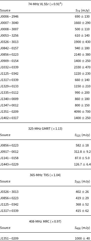
Notes.
 ${}^{\rm a}$
The flux density calibration uncertainty was also increased by 5% following the recommendation presented in Section 5.3 in Lane et al. (Reference Lane, Cotton, van Velzen, Clarke, Kassim, Helmboldt, Lazio and Cohen2014). References: Lane et al. (Reference Lane, Cotton, van Velzen, Clarke, Kassim, Helmboldt, Lazio and Cohen2014, VLSSr), Mauch et al. (Reference Mauch, Klöckner, Rawlings, Jarvis, Hardcastle, Obreschkow, Saikia and Thompson2013, GMRT), Douglas et al. (Reference Douglas, Bash, Bozyan, Torrence and Wolfe1996, TXS) and Large et al. (Reference Large, Mills, Little, Crawford and Sutton1981, Reference Large, Cram and Burgess1991, MRC).
${}^{\rm a}$
The flux density calibration uncertainty was also increased by 5% following the recommendation presented in Section 5.3 in Lane et al. (Reference Lane, Cotton, van Velzen, Clarke, Kassim, Helmboldt, Lazio and Cohen2014). References: Lane et al. (Reference Lane, Cotton, van Velzen, Clarke, Kassim, Helmboldt, Lazio and Cohen2014, VLSSr), Mauch et al. (Reference Mauch, Klöckner, Rawlings, Jarvis, Hardcastle, Obreschkow, Saikia and Thompson2013, GMRT), Douglas et al. (Reference Douglas, Bash, Bozyan, Torrence and Wolfe1996, TXS) and Large et al. (Reference Large, Mills, Little, Crawford and Sutton1981, Reference Large, Cram and Burgess1991, MRC).
The radio data presented in Tables 2 and 4 are from surveys that are not always tied to the same flux density scale. We return to this topic in Section 5.4, as it is an important consideration for the modelling of the broadband radio spectra of our sample. However, for the comparison between the 147.5-MHz TGSS and 151-MHz GLEAM flux densities described below in Section 5.2, we note that we have used rescaled TGSS flux densities from Hurley-Walker (Reference Hurley-Walker2017); these measurements are reported in Table 2. The average multiplicative correction factor applied for the sources in our sample is 0.97, with minimum and maximum values of 0.79 and 1.20, respectively. The rescaling moves the TGSS flux densities onto the flux density scale of Baars et al. (Reference Baars, Genzel, Pauliny-Toth and Witzel1977) that was used to calibrate GLEAM, rather than the Scaife & Heald (Reference Scaife and Heald2012) scale used by Intema et al. (Reference Intema, Jagannathan, Mooley and Frail2017) for the main TGSS catalogue. It also corrects for position-dependent flux density scale variations in TGSS.
There are three sources in the sample with one or more non-detections at the
 $3\sigma$
level: J0034
$3\sigma$
level: J0034
 $-$
3112 (843 MHz), J1521
$-$
3112 (843 MHz), J1521
 $-$
0104 (8.8 GHz), and J2311
$-$
0104 (8.8 GHz), and J2311
 $-$
3359 (843 MHz, 1.4 GHz, and 3 GHz). For J0034
$-$
3359 (843 MHz, 1.4 GHz, and 3 GHz). For J0034
 $-$
3112 and J1521
$-$
3112 and J1521
 $-$
0104, we made use of a technique often used when studying the light curves of radio transients (e.g. Swinbank et al. Reference Swinbank2015): rather than including upper limits in the analysis described below, we instead measured the flux density from a forced point-source fit at the target location using imfit in miriad. This ensured the consistency of the characteristics of the data points, rather than a combination of detections and upper limits. The flux densities from these fits are
$-$
0104, we made use of a technique often used when studying the light curves of radio transients (e.g. Swinbank et al. Reference Swinbank2015): rather than including upper limits in the analysis described below, we instead measured the flux density from a forced point-source fit at the target location using imfit in miriad. This ensured the consistency of the characteristics of the data points, rather than a combination of detections and upper limits. The flux densities from these fits are
 $S_{843} = 9.0 \pm 3.3$
mJy for J0034
$S_{843} = 9.0 \pm 3.3$
mJy for J0034
 $-$
3112 and
$-$
3112 and
 $S_{8800} = 0.14 \pm 0.06$
mJy for J1521
$S_{8800} = 0.14 \pm 0.06$
mJy for J1521
 $-$
0104. Both of these flux densities are consistent with the formal
$-$
0104. Both of these flux densities are consistent with the formal
 $3\sigma$
upper limits (
$3\sigma$
upper limits (
 ${<}10$
and
${<}10$
and
 ${<}0.2\ \mathrm{mJy\, beam}^{-1}$
, respectively). For J2311
${<}0.2\ \mathrm{mJy\, beam}^{-1}$
, respectively). For J2311
 $-$
3359, the SUMSS and NVSS upper limits are not significantly constraining, and we therefore excluded them from our analysis. However, for the VLASS data point, we also measured the flux density from a forced fit:
$-$
3359, the SUMSS and NVSS upper limits are not significantly constraining, and we therefore excluded them from our analysis. However, for the VLASS data point, we also measured the flux density from a forced fit:
 $S_{3000} = 0.18 \pm 0.13$
mJy. This measurement is consistent with the formal
$S_{3000} = 0.18 \pm 0.13$
mJy. This measurement is consistent with the formal
 $3\sigma$
upper limit (
$3\sigma$
upper limit (
 ${<}0.38\ \mathrm{mJy\, beam}^{-1}$
) to within the
${<}0.38\ \mathrm{mJy\, beam}^{-1}$
) to within the
 $2\sigma$
error on the forced-fit value.
$2\sigma$
error on the forced-fit value.
For J0856
 $+$
0223 and J0917
$+$
0223 and J0917
 $-$
0012, these sources were analysed in detail in D20, Drouart et al. (Reference Drouart2021) and Seymour et al. (Reference Seymour2022) over a wider frequency range than is considered here. We report radio properties for these two sources in Tables 2 and 4, but only over the same frequency range as for the other sources in the sample.
$-$
0012, these sources were analysed in detail in D20, Drouart et al. (Reference Drouart2021) and Seymour et al. (Reference Seymour2022) over a wider frequency range than is considered here. We report radio properties for these two sources in Tables 2 and 4, but only over the same frequency range as for the other sources in the sample.
5.2. Comparison of radio flux densities from data sets matched or closely spaced in observing frequency
To assess the reliability of the radio flux densities, we compared several of our data sets: FIRST and NVSS, SUMSS and RACS, and GLEAM and TGSS. Moreover, as our sample was selected using the criterion LAS
 ${\leq}5^{\prime\prime}$
, there was the possibility that one or more very compact components in a given source had resulted in significant variability between the epochs of the surveys used in the three comparisons listed above. Variability resulting from refractive interstellar scintillation (Shapirovskaya Reference Shapirovskaya1978; Rickett, Coles, & Bourgois Reference Rickett, Coles and Bourgois1984; Rickett Reference Rickett1986, Reference Rickett1990) has been observed often at frequencies over the range that we are considering here (e.g. Hunstead Reference Hunstead1972; Gaensler & Hunstead Reference Gaensler and Hunstead2000; Bannister et al. Reference Bannister, Murphy, Gaensler, Hunstead and Chatterjee2011; Ofek & Frail Reference Ofek and Frail2011; Bell et al. Reference Bell2019; Hajela et al. Reference Hajela, Mooley, Intema and Frail2019; Ross et al. Reference Ross2021; Murphy et al. Reference Murphy2021; but see Koay et al. Reference Koay2012 for the case of high-redshift AGN). Other possibilities include intrinsic variability from a compact core and/or jet component (e.g. Mooley et al. Reference Mooley2016; Nyland et al. Reference Nyland2020; Ross et al. Reference Ross2021; Wołowska et al. Reference Wołowska2021) or a combination of both refractive scintillation and intrinsic variability, the former occurring on shorter timescales (e.g. Rickett, Lazio, & Ghigo Reference Rickett, Lazio and Ghigo2006; Bhandari et al. Reference Bhandari2018; Sarbadhicary et al. Reference Sarbadhicary2021).
${\leq}5^{\prime\prime}$
, there was the possibility that one or more very compact components in a given source had resulted in significant variability between the epochs of the surveys used in the three comparisons listed above. Variability resulting from refractive interstellar scintillation (Shapirovskaya Reference Shapirovskaya1978; Rickett, Coles, & Bourgois Reference Rickett, Coles and Bourgois1984; Rickett Reference Rickett1986, Reference Rickett1990) has been observed often at frequencies over the range that we are considering here (e.g. Hunstead Reference Hunstead1972; Gaensler & Hunstead Reference Gaensler and Hunstead2000; Bannister et al. Reference Bannister, Murphy, Gaensler, Hunstead and Chatterjee2011; Ofek & Frail Reference Ofek and Frail2011; Bell et al. Reference Bell2019; Hajela et al. Reference Hajela, Mooley, Intema and Frail2019; Ross et al. Reference Ross2021; Murphy et al. Reference Murphy2021; but see Koay et al. Reference Koay2012 for the case of high-redshift AGN). Other possibilities include intrinsic variability from a compact core and/or jet component (e.g. Mooley et al. Reference Mooley2016; Nyland et al. Reference Nyland2020; Ross et al. Reference Ross2021; Wołowska et al. Reference Wołowska2021) or a combination of both refractive scintillation and intrinsic variability, the former occurring on shorter timescales (e.g. Rickett, Lazio, & Ghigo Reference Rickett, Lazio and Ghigo2006; Bhandari et al. Reference Bhandari2018; Sarbadhicary et al. Reference Sarbadhicary2021).
5.2.1. Comparison at mid frequencies
For the EQU sources, we compared the 1.4-GHz NVSS and FIRST flux densities. As our sources are selected to be compact in the radio, the difference in the angular resolutions of NVSS and FIRST for these particular targets (
 $45^{\prime\prime} \times 45^{\prime\prime}$
for NVSS and
$45^{\prime\prime} \times 45^{\prime\prime}$
for NVSS and
 $6.\!^{\prime\prime} 4 \times 5.\!^{\prime\prime}4$
with BPA
$6.\!^{\prime\prime} 4 \times 5.\!^{\prime\prime}4$
with BPA
 $= 0^\circ$
for FIRST) should not result in a significant difference between the two flux densities for a given source, i.e. the NVSS flux densities should not be systematically brighter as a result of extended emission being resolved out in FIRST. We determined that the NVSS/FIRST flux density ratio has a mean and standard error of the mean of 0.99 and 0.02, respectively; the minimum and maximum values are 0.82 (J1040
$= 0^\circ$
for FIRST) should not result in a significant difference between the two flux densities for a given source, i.e. the NVSS flux densities should not be systematically brighter as a result of extended emission being resolved out in FIRST. We determined that the NVSS/FIRST flux density ratio has a mean and standard error of the mean of 0.99 and 0.02, respectively; the minimum and maximum values are 0.82 (J1040
 $+$
0150) and 1.33 (J1037
$+$
0150) and 1.33 (J1037
 $-$
0325). Inspecting the uncertainties associated with individual NVSS and FIRST flux density measurements, J1037
$-$
0325). Inspecting the uncertainties associated with individual NVSS and FIRST flux density measurements, J1037
 $-$
0325 and J1040
$-$
0325 and J1040
 $+$
0150 are the only sources where the difference from unity for the NVSS/FIRST flux density ratio is more than
$+$
0150 are the only sources where the difference from unity for the NVSS/FIRST flux density ratio is more than
 $3\sigma$
. It is beyond the scope of this paper to thoroughly consider all possible systematic effects that may result in a statistically significant offset. Any significant difference could instead indicate mild variability. For J1037
$3\sigma$
. It is beyond the scope of this paper to thoroughly consider all possible systematic effects that may result in a statistically significant offset. Any significant difference could instead indicate mild variability. For J1037
 $-$
0325, it is also possible that some extended emission has been resolved out in FIRST, which may in turn suggest that this source is not as compact as indicated by both the FIRST and VLASS data.
$-$
0325, it is also possible that some extended emission has been resolved out in FIRST, which may in turn suggest that this source is not as compact as indicated by both the FIRST and VLASS data.
We carried out a similar comparison for those sources with data in both SUMSS at 843 MHz (angular resolution
 $45 \csc{\lvert \delta \rvert}^{\prime\prime} \times 45^{\prime\prime}$
with BPA
$45 \csc{\lvert \delta \rvert}^{\prime\prime} \times 45^{\prime\prime}$
with BPA
 $= 0^\circ$
) and RACS (angular resolution
$= 0^\circ$
) and RACS (angular resolution
 $25^{\prime\prime} \times 25^{\prime\prime}$
) at 887.5 MHz. For a source with a canonical spectral index of
$25^{\prime\prime} \times 25^{\prime\prime}$
) at 887.5 MHz. For a source with a canonical spectral index of
 $\alpha = -0.7$
, the expected SUMSS/RACS flux density ratio is 1.037; similarly, the expected flux density ratio is 1.069 for
$\alpha = -0.7$
, the expected SUMSS/RACS flux density ratio is 1.037; similarly, the expected flux density ratio is 1.069 for
 $\alpha = -1.3$
. We calculated a mean SUMSS/RACS flux density ratio of 1.01, with a standard error of the mean of 0.04. Hale et al. (Reference Hale2021) also found an excellent agreement between SUMSS and RACS from a more general comparison of these two surveys. The minimum and maximum ratios from our comparison are 0.71 (J2330
$\alpha = -1.3$
. We calculated a mean SUMSS/RACS flux density ratio of 1.01, with a standard error of the mean of 0.04. Hale et al. (Reference Hale2021) also found an excellent agreement between SUMSS and RACS from a more general comparison of these two surveys. The minimum and maximum ratios from our comparison are 0.71 (J2330
 $-$
3237) and 1.26 (J0002
$-$
3237) and 1.26 (J0002
 $-$
3514). J2330
$-$
3514). J2330
 $-$
3237 is the only source for which there is evidence of a discrepancy at the
$-$
3237 is the only source for which there is evidence of a discrepancy at the
 $> 3\sigma$
level between the measured and expected SUMSS/RACS flux density ratios (note that J1037
$> 3\sigma$
level between the measured and expected SUMSS/RACS flux density ratios (note that J1037
 $-$
0325 and J1040
$-$
0325 and J1040
 $+$
0150 discussed above are not within the SUMSS survey footprint). Inspecting the broadband radio data for this source (Figure 2), there is a suggestion that the RACS flux density might be slightly overestimated. A comparison of the FIRST and NVSS flux densities was not possible for J2330
$+$
0150 discussed above are not within the SUMSS survey footprint). Inspecting the broadband radio data for this source (Figure 2), there is a suggestion that the RACS flux density might be slightly overestimated. A comparison of the FIRST and NVSS flux densities was not possible for J2330
 $-$
3237 as it is not within the FIRST survey footprint.
$-$
3237 as it is not within the FIRST survey footprint.
5.2.2. Comparison at low frequencies
We compared the rescaled TGSS data at 147.5 MHz with the fitted 151-MHz flux densities from GLEAM. For our sample, the angular resolutions of TGSS and GLEAM are
 $25\sec\!(\delta-19^\circ)^{\prime\prime} \times 25^{\prime\prime}$
(
$25\sec\!(\delta-19^\circ)^{\prime\prime} \times 25^{\prime\prime}$
(
 $\mathrm{BPA} = 0^\circ$
) and
$\mathrm{BPA} = 0^\circ$
) and
 $2.^{\!\!\prime}5 \times 2.^{\!\!\prime} 2\sec\!(\delta + 26.\!\!^\circ7)$
(BPA
$2.^{\!\!\prime}5 \times 2.^{\!\!\prime} 2\sec\!(\delta + 26.\!\!^\circ7)$
(BPA
 $= 0^\circ$
or
$= 0^\circ$
or
 $90^\circ$
), respectively, with the latter resolution at 154 MHz. For a source with
$90^\circ$
), respectively, with the latter resolution at 154 MHz. For a source with
 $\alpha = -0.7$
, the expected GLEAM/TGSS flux density ratio is 0.984 (0.970 for
$\alpha = -0.7$
, the expected GLEAM/TGSS flux density ratio is 0.984 (0.970 for
 $\alpha = -1.3$
). We found that the mean and standard error of the mean for the GLEAM/TGSS flux density ratio are 1.08 and 0.03, respectively; the minimum and maximum values are 0.83 (J0239
$\alpha = -1.3$
). We found that the mean and standard error of the mean for the GLEAM/TGSS flux density ratio are 1.08 and 0.03, respectively; the minimum and maximum values are 0.83 (J0239
 $-$
3043) and 1.65 (J0240
$-$
3043) and 1.65 (J0240
 $-$
3206). Therefore, there is a suggestion that the fitted GLEAM flux densities are slightly overestimated on average or that the rescaled TGSS flux densities are slightly underestimated, with the caveat that this is not a fully like-to-like comparison (i.e. we are comparing a fitted 151-MHz flux density determined using the full bandwidth of GLEAM with a single 147.5-MHz measurement determined over a much narrower bandwidth). There are no sources where the measured and expected GLEAM/TGSS flux density ratios differ at the
$-$
3206). Therefore, there is a suggestion that the fitted GLEAM flux densities are slightly overestimated on average or that the rescaled TGSS flux densities are slightly underestimated, with the caveat that this is not a fully like-to-like comparison (i.e. we are comparing a fitted 151-MHz flux density determined using the full bandwidth of GLEAM with a single 147.5-MHz measurement determined over a much narrower bandwidth). There are no sources where the measured and expected GLEAM/TGSS flux density ratios differ at the
 $> 3\sigma$
level.
$> 3\sigma$
level.
In addition, six of our sources were included in the low-frequency GLEAM spectral variability study by Ross et al. (Reference Ross2021): J0007
 $-$
3040, J0008
$-$
3040, J0008
 $-$
3007, J0108
$-$
3007, J0108
 $-$
3501, J0301
$-$
3501, J0301
 $-$
3132, J0326
$-$
3132, J0326
 $-$
3013 and J2326
$-$
3013 and J2326
 $-$
3028. However, none were identified as being variable between the two GLEAM epochs, separated by 1 year.
$-$
3028. However, none were identified as being variable between the two GLEAM epochs, separated by 1 year.
5.3. Overlay plots
In Figure 2, we present
 $K_{\rm s}$
-band/radio overlay plots for the sources in our sample. We show contours from our highest-resolution radio data sets, i.e. FIRST, VLASS (angular resolution
$K_{\rm s}$
-band/radio overlay plots for the sources in our sample. We show contours from our highest-resolution radio data sets, i.e. FIRST, VLASS (angular resolution
 ${\approx} 2 .\!^{\prime\prime} 5$
) and the ATCA 5.5- and 9-GHz data from the 6A array configuration observations. The deepest
${\approx} 2 .\!^{\prime\prime} 5$
) and the ATCA 5.5- and 9-GHz data from the 6A array configuration observations. The deepest
 $K_{\rm s}$
-band image available for a given source has been used (i.e. from VIKING, SHARKS or HAWK-I). Note, however, that we do not include J0856
$K_{\rm s}$
-band image available for a given source has been used (i.e. from VIKING, SHARKS or HAWK-I). Note, however, that we do not include J0856
 $+$
0023 and J0917
$+$
0023 and J0917
 $-$
0012, which have been analysed extensively elsewhere (D20; Drouart et al. Reference Drouart2021; Seymour et al. Reference Seymour2022). For the overlay plots, a summary of the
$-$
0012, which have been analysed extensively elsewhere (D20; Drouart et al. Reference Drouart2021; Seymour et al. Reference Seymour2022). For the overlay plots, a summary of the
 $K_{\rm s}$
-band host galaxy magnitudes or lower limits and the lowest radio contour levels used can be found in Table 5.
$K_{\rm s}$
-band host galaxy magnitudes or lower limits and the lowest radio contour levels used can be found in Table 5.
The host galaxies of J0133
 $-$
3056 and J0842
$-$
3056 and J0842
 $-$
0157 are detected in the HAWK-I
$-$
0157 are detected in the HAWK-I
 $K_{\rm s}$
-band images. Otherwise, any possible host galaxy detections in the VIKING or SHARKS images (e.g. for J1329
$K_{\rm s}$
-band images. Otherwise, any possible host galaxy detections in the VIKING or SHARKS images (e.g. for J1329
 $+$
0133) are tentative at best and below a
$+$
0133) are tentative at best and below a
 $5\sigma$
brightest pixel value, which indeed is why the sources are included in our sample (Section 2.2.3).
$5\sigma$
brightest pixel value, which indeed is why the sources are included in our sample (Section 2.2.3).
Table 5. Summary of the
 $K_{\rm s}$
-band images and lowest radio contour levels used in the overlay plots in Figure 2. The reported radio contour levels are usually
$K_{\rm s}$
-band images and lowest radio contour levels used in the overlay plots in Figure 2. The reported radio contour levels are usually
 $5\sigma$
, but in a handful of cases they are either
$5\sigma$
, but in a handful of cases they are either
 $3\sigma$
or
$3\sigma$
or
 $4\sigma$
. We also report the
$4\sigma$
. We also report the
 $K_{\rm s}$
-band host galaxy magnitudes (limits at the
$K_{\rm s}$
-band host galaxy magnitudes (limits at the
 $5\sigma$
level); see Section 3 for further details.
$5\sigma$
level); see Section 3 for further details.

Notes.
 ${}^{\rm a}$
Not corrected using the 1/0.87 scaling factor discussed in Section 5.1.
${}^{\rm a}$
Not corrected using the 1/0.87 scaling factor discussed in Section 5.1.
 ${}^{\rm b} 3\sigma$
contour.
${}^{\rm b} 3\sigma$
contour.
 ${}^{\rm c} 4\sigma$
contour.
${}^{\rm c} 4\sigma$
contour.
Given our LAS
 ${\leq}5 ^{\prime\prime}$
selection criterion and the angular resolutions of the VLASS and ATCA data (which are similar for the SGP sources), it is not particularly surprising that all but one of our sources have radio morphologies that can be classified as one of the following: single component, incipient double or resolved double. The one exception is the triple source J0309
${\leq}5 ^{\prime\prime}$
selection criterion and the angular resolutions of the VLASS and ATCA data (which are similar for the SGP sources), it is not particularly surprising that all but one of our sources have radio morphologies that can be classified as one of the following: single component, incipient double or resolved double. The one exception is the triple source J0309
 $-$
3526. Offsets between the VLASS and ATCA centroids are within the astrometric uncertainties of the VLASS quick-look images (up to
$-$
3526. Offsets between the VLASS and ATCA centroids are within the astrometric uncertainties of the VLASS quick-look images (up to
 ${\approx} 1^{\prime\prime}$
; Lacy et al. Reference Lacy2019). Phase errors remaining in the VLASS maps can lead to erroneous extension visible in the overlay plots (e.g. for J0301
${\approx} 1^{\prime\prime}$
; Lacy et al. Reference Lacy2019). Phase errors remaining in the VLASS maps can lead to erroneous extension visible in the overlay plots (e.g. for J0301
 $-$
3132 and J0326
$-$
3132 and J0326
 $-$
3013), and care must be taken interpreting the radio morphology at 3 GHz (see Lacy et al. Reference Lacy2019 for further details).
$-$
3013), and care must be taken interpreting the radio morphology at 3 GHz (see Lacy et al. Reference Lacy2019 for further details).
Further information can be found in the notes on individual sources in Section 5.5.
5.4. Radio spectral modelling
The radio data for each source in our sample spans a maximum frequency range of 74 MHz–9 GHz, with flux density measurements at up to 29 different frequencies. We were therefore able to explore the broadband radio spectral properties of our sample, which could then be compared with the GLEAM-only
 $\alpha$
–
$\alpha$
–
 $\beta$
fitting that was used as part of the sample selection (Section 2.2.2). For each source for which we present an overlay plot in Figure 2, we have also plotted the corresponding observed-frame broadband radio spectrum in the right-hand column of this figure. Overlaid on each spectrum is the preferred model: either a single or double power law. Radio spectra of particular interest are discussed in the notes on individual sources in Section 5.5, followed by further discussion in Sections 6.1 and 6.2.
$\beta$
fitting that was used as part of the sample selection (Section 2.2.2). For each source for which we present an overlay plot in Figure 2, we have also plotted the corresponding observed-frame broadband radio spectrum in the right-hand column of this figure. Overlaid on each spectrum is the preferred model: either a single or double power law. Radio spectra of particular interest are discussed in the notes on individual sources in Section 5.5, followed by further discussion in Sections 6.1 and 6.2.
For J0856
 $+$
0223 and J0917
$+$
0223 and J0917
 $-$
0012, radio spectra over a wider frequency range were presented in D20, Drouart et al. (Reference Drouart2021) and Seymour et al. (Reference Seymour2022). We do not show spectra for these sources in Figure 2, but instead analyse these sources later in this paper in Section 6.2 and Figure 3.
$-$
0012, radio spectra over a wider frequency range were presented in D20, Drouart et al. (Reference Drouart2021) and Seymour et al. (Reference Seymour2022). We do not show spectra for these sources in Figure 2, but instead analyse these sources later in this paper in Section 6.2 and Figure 3.
We now describe the steps taken to construct the broadband radio spectra and carry out the spectral modelling.
5.4.1. Flux density scale corrections
Before we could model the broadband radio spectrum of each source, we first had to consider the fact that the radio data presented in Tables 2 and 5 were calibrated using a variety of flux density scales. Descriptions of these scales as well as relevant summaries and overviews can be found in the following references: Wyllie (Reference Wyllie1969a, b), Wills (Reference Wills1973), Roger, Costain, & Bridle (Reference Roger, Costain and Bridle1973), Baars et al. (Reference Baars, Genzel, Pauliny-Toth and Witzel1977), Hunstead (Reference Hunstead1991), Reynolds (Reference Reynolds1994), Douglas et al. (Reference Douglas, Bash, Bozyan, Torrence and Wolfe1996), Scaife & Heald (Reference Scaife and Heald2012), Mauch et al. (Reference Mauch, Klöckner, Rawlings, Jarvis, Hardcastle, Obreschkow, Saikia and Thompson2013), Hurley-Walker et al. (Reference Hurley-Walker2017), Hurley-Walker (Reference Hurley-Walker2017) and Perley & Butler (Reference Perley and Butler2017). In particular, given that GLEAM is tied to the Baars et al. (Reference Baars, Genzel, Pauliny-Toth and Witzel1977) flux density scale, we chose to rescale our other data sets, if required, to this scale. While this scale is known to become less accurate at low frequencies (e.g. discussion in Rees Reference Rees1990, Scaife & Heald Reference Scaife and Heald2012, Hurley-Walker et al. Reference Hurley-Walker2017 and Perley & Butler Reference Perley and Butler2017), to first order this should not affect the spectral modelling presented below.
As described above in Section 5.1, we used the rescaled TGSS flux densities from Hurley-Walker (Reference Hurley-Walker2017). Our ATCA data are also tied to the Baars et al. (Reference Baars, Genzel, Pauliny-Toth and Witzel1977) scale, as are the RACS, FIRST and NVSS flux densities.Footnote h It was not deemed necessary to rescale the SUMSS data given the agreement between SUMSS and RACS (Section 5.2.1 and Hale et al. Reference Hale2021); the consistency between the Baars et al. (Reference Baars, Genzel, Pauliny-Toth and Witzel1977) and Perley & Butler (Reference Perley and Butler2017) scales at 3 GHz meant that a correction was not needed for VLASS either.
The rescaled VLSSr, 325-MHz GMRT, TXS and MRC flux densities, as well as the multiplicative correction factors used, can be found in Table 4. For VLSSr and TXS, these factors were directly available in the references for these surveys (Douglas et al. Reference Douglas, Bash, Bozyan, Torrence and Wolfe1996; Lane et al. Reference Lane, Cotton, van Velzen, Clarke, Kassim, Helmboldt, Lazio and Cohen2014); we also increased the VLSSr calibration uncertainty by 5% as recommended by Lane et al. (Reference Lane, Cotton, van Velzen, Clarke, Kassim, Helmboldt, Lazio and Cohen2014) when rescaling the catalogued flux densities, which are tied to the Scaife & Heald (Reference Scaife and Heald2012) flux density scale. For the GMRT data, the correction factor could be determined using the information in both Mauch et al. (Reference Mauch, Klöckner, Rawlings, Jarvis, Hardcastle, Obreschkow, Saikia and Thompson2013) and Perley & Butler (Reference Perley and Butler2017), and for the MRC a correction factor is available in Baars et al. (Reference Baars, Genzel, Pauliny-Toth and Witzel1977).
With all of the radio data on a consistent flux density scale, we could then fit each broadband spectrum.
5.4.2. Modelling the data
As in D20, we fitted a single, double and triple power law to each spectrum. We made use of the emcee (Foreman-Mackey et al. Reference Foreman-Mackey2013a, b) and george (Ambikasaran et al. Reference Ambikasaran, Foreman-Mackey, Greengard, Hogg and O’Neil2015; Foreman-Mackey Reference Foreman-Mackey2015) modules in python, so as to carry out a Markov Chain Monte Carlo analysis of the parameter space. A single-power-law fit was defined as follows:
 \begin{equation}S_{\nu} = N\!\left(\frac{\nu}{\nu_{0}}\right)^{\alpha},\end{equation}
where N is a constant,
 $\alpha$
the spectral index across the observed-frequency range, and
$\alpha$
the spectral index across the observed-frequency range, and
 $\nu_{0}$
the reference frequency, which we chose to be 1000 MHz. Thus, N is the fitted flux density at 1000 MHz for the single-power-law fit. For the smoothly varying double-power-law fit,
$\nu_{0}$
the reference frequency, which we chose to be 1000 MHz. Thus, N is the fitted flux density at 1000 MHz for the single-power-law fit. For the smoothly varying double-power-law fit,
 \begin{equation}S_{\nu} = N\!\left(\frac{\nu}{\nu_{0}}\right)^{\alpha_{\rm l}} \times \left[1 + \left(\frac{\nu}{\nu_{\rm b}}\right)^{\lvert\alpha_{\rm h} - \alpha_{\rm l}\rvert}\right]^{\mathrm{sgn}{(\alpha_{\rm h} - \alpha_{\rm l})}},\end{equation}
where
 $\alpha_{\rm l}$
and
$\alpha_{\rm l}$
and
 $\alpha_{\rm h}$
are the spectral indices either side of the break frequency
$\alpha_{\rm h}$
are the spectral indices either side of the break frequency
 $\nu_{\rm b}$
and
$\nu_{\rm b}$
and
 $\mathrm{sgn}{}$
the signum function. Lastly, the smoothly varying triple-power-law fit was of the form
$\mathrm{sgn}{}$
the signum function. Lastly, the smoothly varying triple-power-law fit was of the form
 \begin{align}S_{\nu} =\, & N\!\left(\frac{\nu}{\nu_{0}}\right)^{\alpha_{\rm l}} \times \left[1 + \left(\frac{\nu}{\nu_{\rm bl}}\right)^{\lvert\alpha_{\rm m} - \alpha_{\rm l}\rvert}\right]^{\mathrm{sgn}{(\alpha_{\rm m} - \alpha_{\rm l})}} \nonumber\\[4pt]& \times \left[1 + \left(\frac{\nu}{\nu_{\rm bh}}\right)^{\lvert\alpha_{\rm h} - \alpha_{\rm m}\rvert}\right]^{\mathrm{sgn}{(\alpha_{\rm h} - \alpha_{\rm m})}},\end{align}
where
 $\alpha_{\rm l}$
and
$\alpha_{\rm l}$
and
 $\alpha_{\rm m}$
are the spectral indices either side of the lower break frequency
$\alpha_{\rm m}$
are the spectral indices either side of the lower break frequency
 $\nu_{\rm bl}$
and similarly for the spectral indices
$\nu_{\rm bl}$
and similarly for the spectral indices
 $\alpha_{\rm m}$
and
$\alpha_{\rm m}$
and
 $\alpha_{\rm h}$
as well as the higher break frequency
$\alpha_{\rm h}$
as well as the higher break frequency
 $\nu_{\rm bh}$
.
$\nu_{\rm bh}$
.
Table 6. Non-informative priors for each of the parameters in Equations (4)–(6). Section 5.4 describes how we modelled the broadband radio spectra.

The data were fitted with input units of MHz and mJy. We used non-informative priors for each of the parameters in Equations (4)–(6); the priors are listed in Table 6. The priors were chosen such that we assumed a triple-power-law fit with a low-frequency turnover (that could result from synchrotron self-absorption and/or free–free absorption). For both the break frequency in the double-power-law fit and the higher break frequency in the triple-power-law fit, the prior was sufficiently general such that we could model spectral steepening at higher frequencies due to one or more energy loss mechanisms, or high-frequency spectral flattening due to a radio core component beginning to dominate over the lobe emission.
When fitting the data, the uncertainty for each GLEAM flux density was calculated by combining the fitting and absolute calibration uncertainties, the latter being 8% for all of the sources in our sample (Hurley-Walker et al. Reference Hurley-Walker2017; Franzen et al. Reference Franzen, Hurley-Walker, White, Hancock, Seymour, Kapińska, Staveley-Smith and Wayth2021). Furthermore, it was necessary to take into account the correlations that exist between the GLEAM sub-bands, so as to avoid erroneous fits (see discussion in Hurley-Walker et al. Reference Hurley-Walker2017). To do so, we used a blocked Matérn covariance function for the GLEAM flux densities (Rasmussen & Williams Reference Rasmussen and Williams2006).
The preferred model for each radio spectrum was determined using the sample-size-corrected Akaike Information Criterion (AICc; Akaike Reference Akaike1974; Burnham & Anderson Reference Burnham and Anderson2002). In particular,
 \begin{equation}{\rm AICc} = \chi^2 + 2k + \frac{ 2k(k+1)}{n - k - 1},\end{equation}
where n and k are the number of data points and free parameters, respectively, and
 $\chi^2$
is the standard goodness-of-fit statistic. For all possible realisations from the emcee fitting, we determined the minimum value of AICc,
$\chi^2$
is the standard goodness-of-fit statistic. For all possible realisations from the emcee fitting, we determined the minimum value of AICc,
 $\min$
(AICc), for each of the possible three models. We then selected the preferred model by using the standard convention of examining the difference
$\min$
(AICc), for each of the possible three models. We then selected the preferred model by using the standard convention of examining the difference
 \begin{align}\Delta{\rm AICc} & = \min\!({\rm AICc})_{i}\nonumber\\&\quad - \min\{\min(\rm{AICc})_{\rm SPL}, \min\!({\rm AICc})_{\rm DPL}, \min\!({\rm AICc})_{\rm TPL}\},\end{align}
where the subscripts SPL, DPL and TPL refer to the single-power-law, double-power-law, and triple-power-law fits, respectively, and the ith model can be one of the three possibilities. Our preferred model first satisfied the condition
 $0 \leq \Delta{\rm AICc} < 4$
and secondly was the model with the fewest free parameters satisfying this condition. Note that this can mean, for example, that a double-power-law fit has the lowest AICc value, but the single power law was selected as the preferred fit because
$0 \leq \Delta{\rm AICc} < 4$
and secondly was the model with the fewest free parameters satisfying this condition. Note that this can mean, for example, that a double-power-law fit has the lowest AICc value, but the single power law was selected as the preferred fit because
 $\Delta{\rm AICc}$
is sufficiently small enough.
$\Delta{\rm AICc}$
is sufficiently small enough.
The fitted model parameters are presented in Table 7. For 34 sources, the preferred model is a double power law, with the remaining 17 sources described by a single power law. The triple power law is not the preferred model for any of the sources (but see Drouart et al. Reference Drouart2021 and Seymour et al. Reference Seymour2022, where the radio emission from J0917
 $-$
0012 was modelled with a triple power law).
$-$
0012 was modelled with a triple power law).
Table 7. Fitted parameters for the broadband radio spectra. We give the preferred model type: SPL for a single power law and DPL for a double power law. The 16th, 50th and 84th percentiles are reported for the marginalised parameter distributions. We also list the parameter values corresponding to the best fit with the smallest value of AICc as well as the reduced chi-squared goodness-of-fit statistic for this model. Further information on the modelling can be found in Section 5.4.

5.4.3. Possible effects of source blending
We also investigated whether the GLEAM
 $\alpha$
–
$\alpha$
–
 $\beta$
selection and broadband spectral fitting could be affected by source blending in GLEAM. While we used a selection criterion of a single NVSS match within
$\beta$
selection and broadband spectral fitting could be affected by source blending in GLEAM. While we used a selection criterion of a single NVSS match within
 $50^{\prime\prime}$
of the GLEAM position (Table 1) so as to preferentially select isolated, compact sources, the GLEAM synthesised beam half width at half maximum (HWHM) generally extends beyond
$50^{\prime\prime}$
of the GLEAM position (Table 1) so as to preferentially select isolated, compact sources, the GLEAM synthesised beam half width at half maximum (HWHM) generally extends beyond
 $50^{\prime\prime}$
, especially so at the lower end of the GLEAM band. There are also some cases where relatively faint, unassociated sources are visible within
$50^{\prime\prime}$
, especially so at the lower end of the GLEAM band. There are also some cases where relatively faint, unassociated sources are visible within
 $50^{\prime\prime}$
in the RACS, VLASS, and/or ATCA radio maps at the various frequencies (Figure 2; also see Section 5.5). These sources are not visible in NVSS due to either source blending in this survey, or they are too faint to have been detected.
$50^{\prime\prime}$
in the RACS, VLASS, and/or ATCA radio maps at the various frequencies (Figure 2; also see Section 5.5). These sources are not visible in NVSS due to either source blending in this survey, or they are too faint to have been detected.
Having inspected the RACS, VLASS and ATCA radio maps with the GLEAM synthesised beam FWHMs across the full frequency range overlaid, in general we are confident that, in the vast majority of cases, any source blending in GLEAM has not affected the accuracy of both the GLEAM
 $\alpha$
–
$\alpha$
–
 $\beta$
selection and broadband spectral fitting. Contributions from unassociated sources should be contained within the GLEAM flux density uncertainties. Similarly, we also considered whether blending is affecting the reliability of our flux density measurements at other frequencies. However, given the discussion and analysis in Section 5.5 of relevant cases of interest, this is unlikely to be a significant effect.
$\beta$
selection and broadband spectral fitting. Contributions from unassociated sources should be contained within the GLEAM flux density uncertainties. Similarly, we also considered whether blending is affecting the reliability of our flux density measurements at other frequencies. However, given the discussion and analysis in Section 5.5 of relevant cases of interest, this is unlikely to be a significant effect.
5.5. Notes on individual sources
In this section, we discuss the overlay plots and/or radio spectra of a number of sources in the sample.
J0007
 $-$
3040: This source is of particular interest, with
$-$
3040: This source is of particular interest, with
 $K_{\rm s} > 23.1$
from SHARKS, a relatively compact radio morphology with LAS
$K_{\rm s} > 23.1$
from SHARKS, a relatively compact radio morphology with LAS
 $=3.\!^{\prime\prime}0$
in both the ATCA and VLASS images, and a double-power-law spectrum with best-fitting spectral indices of
$=3.\!^{\prime\prime}0$
in both the ATCA and VLASS images, and a double-power-law spectrum with best-fitting spectral indices of
 $\alpha_{\rm l} = -1.385$
and
$\alpha_{\rm l} = -1.385$
and
 $\alpha_{\rm h} = -2.75$
. While
$\alpha_{\rm h} = -2.75$
. While
 $\alpha_{\rm l}$
indicates a USS spectrum at frequencies below
$\alpha_{\rm l}$
indicates a USS spectrum at frequencies below
 $\nu_{\rm b} = 1.97$
GHz,
$\nu_{\rm b} = 1.97$
GHz,
 $\alpha_{\rm h}$
is exceptionally steep and relatively well constrained. This source therefore appears to be a promising HzRG candidate; possible scenarios for explaining the properties of the radio spectrum are discussed in Section 6.1. Another possibility is that this source may be an as of yet undetected pulsar, but this seems less likely given the LAS and the fact that there are hints of an incipient double radio morphology for this source.
$\alpha_{\rm h}$
is exceptionally steep and relatively well constrained. This source therefore appears to be a promising HzRG candidate; possible scenarios for explaining the properties of the radio spectrum are discussed in Section 6.1. Another possibility is that this source may be an as of yet undetected pulsar, but this seems less likely given the LAS and the fact that there are hints of an incipient double radio morphology for this source.
We also note that we checked whether emission potentially being resolved out in the ATCA maps could explain at least some of the observed spectral curvature. Adjusting the robust weighting parameter at 5.5 GHz to
 $-$
2 (i.e. close to uniform weighting) gave an image with a very similar resolution to the 9-GHz map generated with a robust weighting parameter of 0.5. The measured 5.5-GHz flux density was not significantly different to the value reported in Table 2. Additionally, a 5.5-GHz map generated with a robust weighting parameter of 2 (i.e. close to natural weighting) also gave a very similar flux density to the value in Table 2.
$-$
2 (i.e. close to uniform weighting) gave an image with a very similar resolution to the 9-GHz map generated with a robust weighting parameter of 0.5. The measured 5.5-GHz flux density was not significantly different to the value reported in Table 2. Additionally, a 5.5-GHz map generated with a robust weighting parameter of 2 (i.e. close to natural weighting) also gave a very similar flux density to the value in Table 2.
J0133
 $-$
3056: This source is an incipient double in VLASS with LAS
$-$
3056: This source is an incipient double in VLASS with LAS
 $= 4.\!^{\prime\prime} 3$
. The likely host galaxy is seen in the HAWK-I
$= 4.\!^{\prime\prime} 3$
. The likely host galaxy is seen in the HAWK-I
 $K_{\rm s}$
-band image close to the peak of the radio emission, with magnitude
$K_{\rm s}$
-band image close to the peak of the radio emission, with magnitude
 $K_{\rm s} = 22.23 \pm 0.08$
.
$K_{\rm s} = 22.23 \pm 0.08$
.
J0309
 $-$
3526: The ATCA 5.5-GHz and VLASS data both suggest a multi-component morphology, perhaps a triple source, although as can be seen in the corresponding panel in Figure 2, the morphologies are not fully consistent between the two frequencies. There is clear extension at 5.5 GHz in the direction of the synthesised beam, almost orthogonal to what appears to be the main axis of the radio emission. Given the VLASS morphology and the fact that we could not phase self-calibrate the 5.5-GHz data due to low S/N, it seems most plausible that the extension at 5.5 GHz in the direction of the synthesised beam is spurious. The spectral index between 5.5 and 9 GHz is extremely steep:
$-$
3526: The ATCA 5.5-GHz and VLASS data both suggest a multi-component morphology, perhaps a triple source, although as can be seen in the corresponding panel in Figure 2, the morphologies are not fully consistent between the two frequencies. There is clear extension at 5.5 GHz in the direction of the synthesised beam, almost orthogonal to what appears to be the main axis of the radio emission. Given the VLASS morphology and the fact that we could not phase self-calibrate the 5.5-GHz data due to low S/N, it seems most plausible that the extension at 5.5 GHz in the direction of the synthesised beam is spurious. The spectral index between 5.5 and 9 GHz is extremely steep:
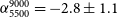 $\alpha^{9000}_{5500} = -2.8 \pm 1.1$
. There is evidence that the accuracy of
$\alpha^{9000}_{5500} = -2.8 \pm 1.1$
. There is evidence that the accuracy of
 $\alpha^{9000}_{5500}$
is affected by diffuse emission being resolved out; this can be seen, for example, by decreasing the robust weighting parameter from 0.5 to
$\alpha^{9000}_{5500}$
is affected by diffuse emission being resolved out; this can be seen, for example, by decreasing the robust weighting parameter from 0.5 to
 $-$
2 (i.e. uniform weighting in the latter case) and reimaging the 5.5-GHz data. Higher S/N data at mid/high frequencies in array configurations with sufficient low-surface-brightness sensitivity are needed for this source.
$-$
2 (i.e. uniform weighting in the latter case) and reimaging the 5.5-GHz data. Higher S/N data at mid/high frequencies in array configurations with sufficient low-surface-brightness sensitivity are needed for this source.
J0842
 $-$
0157: The FIRST and VLASS morphologies are very compact: LAS
$-$
0157: The FIRST and VLASS morphologies are very compact: LAS
 $=1.\!^{\prime\prime}7$
and
$=1.\!^{\prime\prime}7$
and
 $1.\!^{\prime\prime}1$
, respectively. We take the HAWK-I
$1.\!^{\prime\prime}1$
, respectively. We take the HAWK-I
 $K_{\rm s}$
-band source closest to the radio centroid as the host galaxy identification; the magnitude of the host galaxy is
$K_{\rm s}$
-band source closest to the radio centroid as the host galaxy identification; the magnitude of the host galaxy is
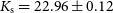 $K_{\rm s} = 22.96 \pm 0.12$
.
$K_{\rm s} = 22.96 \pm 0.12$
.
J0909
 $-$
0154, J1141
$-$
0154, J1141
 $-$
0158 and J1443
$-$
0158 and J1443
 $+$
0229: The best-fitting model for J0909
$+$
0229: The best-fitting model for J0909
 $-$
0154 has significantly flattened at the bottom end of the GLEAM band and would be expected to begin to turn over at frequencies
$-$
0154 has significantly flattened at the bottom end of the GLEAM band and would be expected to begin to turn over at frequencies
 $\lesssim 70$
MHz. J1141
$\lesssim 70$
MHz. J1141
 $-$
0158 and J1443
$-$
0158 and J1443
 $+$
0229 are the only sources in the sample where the best fit peaks and turns over (within the GLEAM band at 205 and 91 MHz, respectively); higher S/N data at the lower GLEAM frequencies are needed to confirm the turnover in each case, however.
$+$
0229 are the only sources in the sample where the best fit peaks and turns over (within the GLEAM band at 205 and 91 MHz, respectively); higher S/N data at the lower GLEAM frequencies are needed to confirm the turnover in each case, however.
J1112
 $+$
0056: There is a second NVSS source
$+$
0056: There is a second NVSS source
 $51.\!^{\prime\prime} 3$
from the GLEAM position (beyond the region shown in the panel for this source in Figure 2) that has a 1.4-GHz flux density that is about 40% of the NVSS flux density of the HzRG candidate (NVSS J111212
$51.\!^{\prime\prime} 3$
from the GLEAM position (beyond the region shown in the panel for this source in Figure 2) that has a 1.4-GHz flux density that is about 40% of the NVSS flux density of the HzRG candidate (NVSS J111212
 $+$
005519 with
$+$
005519 with
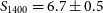 $S_{1400} = 6.7 \pm 0.5$
mJy; cf.
$S_{1400} = 6.7 \pm 0.5$
mJy; cf.
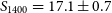 $S_{1400} = 17.1 \pm 0.7$
mJy for the HzRG candidate). Both of these sources have very similar two-point spectral indices
$S_{1400} = 17.1 \pm 0.7$
mJy for the HzRG candidate). Both of these sources have very similar two-point spectral indices
 $\alpha^{1400}_{887.5}$
; if this spectral similarity is also the case at low frequencies, the accuracy of the GLEAM
$\alpha^{1400}_{887.5}$
; if this spectral similarity is also the case at low frequencies, the accuracy of the GLEAM
 $\alpha$
–
$\alpha$
–
 $\beta$
fitting should not be affected significantly. The GLEAM/TGSS flux density ratio in Table 2 is
$\beta$
fitting should not be affected significantly. The GLEAM/TGSS flux density ratio in Table 2 is
 $1.27 \pm 0.15$
; this tentatively suggests that there could be an excess in GLEAM due to source blending, albeit not statistically significant at e.g. the
$1.27 \pm 0.15$
; this tentatively suggests that there could be an excess in GLEAM due to source blending, albeit not statistically significant at e.g. the
 $3\sigma$
level.
$3\sigma$
level.
J1125
 $-$
0342 and J1317
$-$
0342 and J1317
 $+$
0339: These are the USS-selected sources TN J1125
$+$
0339: These are the USS-selected sources TN J1125
 $-$
0342 and TN J1317
$-$
0342 and TN J1317
 $+$
0339, respectively, from De Breuck et al. (Reference De Breuck, van Breugel, Röttgering and Miley2000). Their redshifts remain unknown and the VIKING non-detections are the deepest constraints on their
$+$
0339, respectively, from De Breuck et al. (Reference De Breuck, van Breugel, Röttgering and Miley2000). Their redshifts remain unknown and the VIKING non-detections are the deepest constraints on their
 $K_{\rm s}$
-band magnitudes:
$K_{\rm s}$
-band magnitudes:
 $>21.4$
(J1125
$>21.4$
(J1125
 $-$
0342) and
$-$
0342) and
 $> 21.3$
(J1317
$> 21.3$
(J1317
 $+$
0339).
$+$
0339).
For J1125
 $-$
0342, two sources separated by
$-$
0342, two sources separated by
 $8.\!^{\prime\prime} 3$
are visible in the VLASS Epoch 1 image. The 3-GHz flux density of the southern source is
$8.\!^{\prime\prime} 3$
are visible in the VLASS Epoch 1 image. The 3-GHz flux density of the southern source is
 ${\approx} 1.4$
mJy, a factor of
${\approx} 1.4$
mJy, a factor of
 $\sim$
20 fainter than the much brighter source to the north. J1125
$\sim$
20 fainter than the much brighter source to the north. J1125
 $-$
0342 could therefore be a very asymmetric double, or the fainter source to the south is unrelated. In the case of the former scenario, the angular size would then suggest that the source is too extended to be at a very high redshift. For the purpose of analysis in this paper, we have assumed the latter scenario. Deeper
$-$
0342 could therefore be a very asymmetric double, or the fainter source to the south is unrelated. In the case of the former scenario, the angular size would then suggest that the source is too extended to be at a very high redshift. For the purpose of analysis in this paper, we have assumed the latter scenario. Deeper
 $K_{\rm s}$
-band imaging and higher-resolution radio imaging at e.g. 5.5 and 9 GHz are needed.
$K_{\rm s}$
-band imaging and higher-resolution radio imaging at e.g. 5.5 and 9 GHz are needed.
For J1317
 $+$
0339, it can be seen in Figure 2 that the 365-MHz flux density point is a clear outlier; we did not include this data point when fitting the radio spectrum. The
$+$
0339, it can be seen in Figure 2 that the 365-MHz flux density point is a clear outlier; we did not include this data point when fitting the radio spectrum. The
 $\alpha_{\rm l}$
value in Table 7 implies that the spectrum is not as steep as suggested by the two-point spectral index between the TXS and NVSS surveys. This is the case for J1125
$\alpha_{\rm l}$
value in Table 7 implies that the spectrum is not as steep as suggested by the two-point spectral index between the TXS and NVSS surveys. This is the case for J1125
 $-$
0342 as well, although not to the same extent as for J1317
$-$
0342 as well, although not to the same extent as for J1317
 $+$
0339. We included the 365-MHz data point when fitting the radio spectrum of J1125
$+$
0339. We included the 365-MHz data point when fitting the radio spectrum of J1125
 $-$
0342.
$-$
0342.
J1329
 $+$
0133: There is a hint of a host galaxy identification in the VIKING
$+$
0133: There is a hint of a host galaxy identification in the VIKING
 $K_{\rm s}$
-band image, but the brightest pixel value is only at the
$K_{\rm s}$
-band image, but the brightest pixel value is only at the
 $3.5\sigma$
level (which we do not consider to be a secure detection).
$3.5\sigma$
level (which we do not consider to be a secure detection).
J1335
 $+$
0112: As previously discussed in Section 2.3, this source has a detection in AllWISE: the W1-band magnitude is
$+$
0112: As previously discussed in Section 2.3, this source has a detection in AllWISE: the W1-band magnitude is
 $20.033 \pm 0.130$
(Cutri et al. Reference Cutri2014). The source is not detected in any of the other three longer-wavelength AllWISE bands. The
$20.033 \pm 0.130$
(Cutri et al. Reference Cutri2014). The source is not detected in any of the other three longer-wavelength AllWISE bands. The
 $K_{\rm s}$
-band magnitude is
$K_{\rm s}$
-band magnitude is
 $> 21.2$
(Table 5); the
$> 21.2$
(Table 5); the
 ${\gtrsim} 1.2$
mag break between 2.15 and
${\gtrsim} 1.2$
mag break between 2.15 and
 $3.37\, \unicode{x03BC} \mathrm{m}$
might potentially indicate a redshifted 4000 Å break (i.e.
$3.37\, \unicode{x03BC} \mathrm{m}$
might potentially indicate a redshifted 4000 Å break (i.e.
 $z \gtrsim 4.4$
). The AllWISE W2-band magnitude is
$z \gtrsim 4.4$
). The AllWISE W2-band magnitude is
 $> 19.064$
(
$> 19.064$
(
 $5\sigma$
). Additional follow-up and analysis is needed.
$5\sigma$
). Additional follow-up and analysis is needed.
J1340
 $+$
0009: There is a hint of a host galaxy identification in the VIKING H-band image, but the brightest pixel value is only at the
$+$
0009: There is a hint of a host galaxy identification in the VIKING H-band image, but the brightest pixel value is only at the
 $4.2\sigma$
level (which we do not consider to be a secure detection).
$4.2\sigma$
level (which we do not consider to be a secure detection).
J1351
 $-$
0209: This is the brightest radio source in our sample (by a factor of about three at 151 MHz) with
$-$
0209: This is the brightest radio source in our sample (by a factor of about three at 151 MHz) with
 $S_{151} = 2.44$
Jy. It is also catalogued as the Parkes source PKS B1349
$S_{151} = 2.44$
Jy. It is also catalogued as the Parkes source PKS B1349
 $-$
019 (Wright & Otrupcek Reference Wright and Otrupcek1990). The PKS 2.7- and 5-GHz flux densities from Wright & Otrupcek (Reference Wright and Otrupcek1990) are 130 and 50 mJy, respectively, consistent with the VLASS and ATCA 5.5-GHz data. Given this consistency at very similar frequencies as well as the fact that uncertainties are not reported for these Parkes measurements, we chose not to use the Parkes flux densities in the radio spectrum modelling.
$-$
019 (Wright & Otrupcek Reference Wright and Otrupcek1990). The PKS 2.7- and 5-GHz flux densities from Wright & Otrupcek (Reference Wright and Otrupcek1990) are 130 and 50 mJy, respectively, consistent with the VLASS and ATCA 5.5-GHz data. Given this consistency at very similar frequencies as well as the fact that uncertainties are not reported for these Parkes measurements, we chose not to use the Parkes flux densities in the radio spectrum modelling.
Additionally, Downes et al. (Reference Downes, Peacock, Savage and Carrie1986) reported 1.5- and 4.9-GHz flux densities from their high-resolution VLA data (250 and 60 mJy, respectively); the former is consistent with the NVSS flux density and the latter with both the Parkes 5-GHz and ATCA 5.5-GHz measurements. Again, there is no significant advantage in including these data in our radio spectrum modelling, particularly as it is unclear what the flux density uncertainties are in these cases as well. The radio morphology in the 4.9-GHz VLA map shows two components; the angular extent (
 ${\sim} 2.\!^{\prime\prime}2$
; position angle
${\sim} 2.\!^{\prime\prime}2$
; position angle
 ${\sim}{-}45^\circ$
) is reasonably consistent with the FIRST and VLASS LAS measurement (
${\sim}{-}45^\circ$
) is reasonably consistent with the FIRST and VLASS LAS measurement (
 $2.\!^{\prime\prime}8$
).
$2.\!^{\prime\prime}8$
).
Dunlop et al. (Reference Dunlop, Peacock, Savage, Lilly, Heasley and Simon1989) did not detect the host galaxy in optical imaging; the reported B- and R-band magnitude limits are
 ${\gtrsim} 24$
. The source is listed in Dunlop & Peacock (Reference Dunlop and Peacock1990) as a candidate high-redshift object, but with
${\gtrsim} 24$
. The source is listed in Dunlop & Peacock (Reference Dunlop and Peacock1990) as a candidate high-redshift object, but with
 $K \approx 19.75$
; this is most likely a misidentification or erroneous catalogue entry given that our overlay plot shows no evidence of a
$K \approx 19.75$
; this is most likely a misidentification or erroneous catalogue entry given that our overlay plot shows no evidence of a
 $K_{\rm s}$
-band identification to a much greater depth (
$K_{\rm s}$
-band identification to a much greater depth (
 $ K_{\rm s} > 21.2$
).
$ K_{\rm s} > 21.2$
).
J1521
 $-$
0104: There is a hint of extension in RACS about
$-$
0104: There is a hint of extension in RACS about
 $20^{\prime\prime}$
to the north-west (beyond the region shown in the panel for this source in Figure 2), albeit at a marginal level (
$20^{\prime\prime}$
to the north-west (beyond the region shown in the panel for this source in Figure 2), albeit at a marginal level (
 ${\sim} 3.9\sigma$
). The extension is coincident with the near-infrared source 2MASS J15215337
${\sim} 3.9\sigma$
). The extension is coincident with the near-infrared source 2MASS J15215337
 $-$
0104034, where
$-$
0104034, where
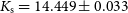 $K_{\rm s} = 14.449 \pm 0.033$
(Cutri et al. Reference Cutri2003). This 2MASS source is
$K_{\rm s} = 14.449 \pm 0.033$
(Cutri et al. Reference Cutri2003). This 2MASS source is
 $22.\!^{\prime\prime}2$
from our HzRG candidate. The possible radio/near-infrared association might then suggest that the HzRG candidate shown in Figure 2 is part of a larger, head–tail source. On the other hand, there is no evidence of similar extension in our other radio data sets. Given that the extended 887.5-MHz radio emission and in turn the radio/near-infrared association is tentative, we regard the source shown in Figure 2 as an HzRG candidate with the requisite compact radio morphology. A deeper
$22.\!^{\prime\prime}2$
from our HzRG candidate. The possible radio/near-infrared association might then suggest that the HzRG candidate shown in Figure 2 is part of a larger, head–tail source. On the other hand, there is no evidence of similar extension in our other radio data sets. Given that the extended 887.5-MHz radio emission and in turn the radio/near-infrared association is tentative, we regard the source shown in Figure 2 as an HzRG candidate with the requisite compact radio morphology. A deeper
 $K_{\rm s}$
-band image would allow us to determine if a host galaxy is associated with this radio source.
$K_{\rm s}$
-band image would allow us to determine if a host galaxy is associated with this radio source.
Thyagarajan et al. (Reference Thyagarajan, Helfand, White and Becker2011) classified J1521
 $-$
0104 as variable at 1.4 GHz based on analysis of the three separate snapshot observations taken for this source as part of FIRST. These authors reported a minimum variability timescale of 8 d. The catalogued FIRST and NVSS flux densities in Table 2 are consistent on a longer timescale (2.1 yr), however.Footnote i Short-timescale variability from a scintillating radio core would rule out that J1521
$-$
0104 as variable at 1.4 GHz based on analysis of the three separate snapshot observations taken for this source as part of FIRST. These authors reported a minimum variability timescale of 8 d. The catalogued FIRST and NVSS flux densities in Table 2 are consistent on a longer timescale (2.1 yr), however.Footnote i Short-timescale variability from a scintillating radio core would rule out that J1521
 $-$
0104 is a component in a larger radio source. Alternatively, the variability may have been due to a scintillating lobe hotspot; this alone would not provide conclusive evidence of the true angular extent of this radio source.
$-$
0104 is a component in a larger radio source. Alternatively, the variability may have been due to a scintillating lobe hotspot; this alone would not provide conclusive evidence of the true angular extent of this radio source.
J2219
 $-$
3312: While this source passed step 8 in Table 1, there is an AllWISE source
$-$
3312: While this source passed step 8 in Table 1, there is an AllWISE source
 $1.\!^{\prime\prime}2$
from the ATCA position. The ATCA centroid is slightly further to the south-south-east than in TGSS (offset
$1.\!^{\prime\prime}2$
from the ATCA position. The ATCA centroid is slightly further to the south-south-east than in TGSS (offset
 $1.\!^{\prime\prime}3$
), and there is also evidence in Figure 2 of a small offset between the ATCA and VLASS centroids. The AllWISE source has W1 and W2 magnitudes of
$1.\!^{\prime\prime}3$
), and there is also evidence in Figure 2 of a small offset between the ATCA and VLASS centroids. The AllWISE source has W1 and W2 magnitudes of
 $20.089 \pm 0.161$
and
$20.089 \pm 0.161$
and
 $20.188 \pm 0.347$
, respectively (Cutri et al. Reference Cutri2014), but is not detected in the longer-wavelength AllWISE bands. The
$20.188 \pm 0.347$
, respectively (Cutri et al. Reference Cutri2014), but is not detected in the longer-wavelength AllWISE bands. The
 $K_{\rm s}$
-band limit is
$K_{\rm s}$
-band limit is
 $> 22.3$
(Table 5); the
$> 22.3$
(Table 5); the
 ${\gtrsim} 2.2$
mag break between
${\gtrsim} 2.2$
mag break between
 $K_{\rm s}$
-band and W1 is larger than for J1335
$K_{\rm s}$
-band and W1 is larger than for J1335
 $+$
0112 discussed above. We regard the AllWISE source as a tentative host galaxy identification; this association needs to be confirmed with follow-up work, particularly deep
$+$
0112 discussed above. We regard the AllWISE source as a tentative host galaxy identification; this association needs to be confirmed with follow-up work, particularly deep
 $K_{\rm s}$
-band imaging.
$K_{\rm s}$
-band imaging.
J2311
 $-$
3359: This source, not selected from our
$-$
3359: This source, not selected from our
 $\alpha$
–
$\alpha$
–
 $\beta$
criteria (as discussed in Section 2.3), has an extremely steep spectrum well described by a single power law with
$\beta$
criteria (as discussed in Section 2.3), has an extremely steep spectrum well described by a single power law with
 $\alpha = -1.842$
. Therefore, J2311
$\alpha = -1.842$
. Therefore, J2311
 $-$
3359 is faint in our higher-frequency images. The source is unresolved in the ATCA data, but the low S/N does not allow an accurate LAS determination. This source is also unresolved in RACS, but we measured an LAS of
$-$
3359 is faint in our higher-frequency images. The source is unresolved in the ATCA data, but the low S/N does not allow an accurate LAS determination. This source is also unresolved in RACS, but we measured an LAS of
 $5.\!^{\prime\prime}6$
in an 887.5-MHz ASKAP early science image of the GAMA-23 field (see Seymour et al. Reference Seymour2020). Such an LAS value falls outside of our LAS
$5.\!^{\prime\prime}6$
in an 887.5-MHz ASKAP early science image of the GAMA-23 field (see Seymour et al. Reference Seymour2020). Such an LAS value falls outside of our LAS
 ${\leq}5^{\prime\prime}$
criterion, but needs to be confirmed with additional radio data. Note in Figure 2 that the VLASS contours are offset from the ATCA contours, but the former are from a line-like artefact in the map.
${\leq}5^{\prime\prime}$
criterion, but needs to be confirmed with additional radio data. Note in Figure 2 that the VLASS contours are offset from the ATCA contours, but the former are from a line-like artefact in the map.
J2330
 $-$
3237: We interpret this source as an asymmetric double with LAS
$-$
3237: We interpret this source as an asymmetric double with LAS
 $4.\!^{\prime\prime}2$
, where the components have significantly different flux densities (the western lobe being much fainter). Using the available high-resolution radio data, the flux densities of the brighter eastern lobe are
$4.\!^{\prime\prime}2$
, where the components have significantly different flux densities (the western lobe being much fainter). Using the available high-resolution radio data, the flux densities of the brighter eastern lobe are
 $6.3 \pm 0.7$
,
$6.3 \pm 0.7$
,
 $3.74 \pm 0.27$
and
$3.74 \pm 0.27$
and
 $2.11 \pm 0.16$
mJy at 3, 5.5 and 9 GHz, respectively. Similarly, the values for the significantly fainter component to the west are
$2.11 \pm 0.16$
mJy at 3, 5.5 and 9 GHz, respectively. Similarly, the values for the significantly fainter component to the west are
 ${<}0.45$
,
${<}0.45$
,
 $0.22 \pm 0.06$
and
$0.22 \pm 0.06$
and
 ${<}0.078$
mJy, respectively (upper limits at the
${<}0.078$
mJy, respectively (upper limits at the
 $3\sigma$
level). Given that the western lobe is detected at 5.5 GHz only, we verified that this source was not spuriously created as a result of our phase-only self-calibration step. The two-point spectral indices are
$3\sigma$
level). Given that the western lobe is detected at 5.5 GHz only, we verified that this source was not spuriously created as a result of our phase-only self-calibration step. The two-point spectral indices are
 $\alpha^{5500}_{3000} = -0.86 \pm 0.22$
and
$\alpha^{5500}_{3000} = -0.86 \pm 0.22$
and
 $\alpha^{9000}_{5500} = -1.16 \pm 0.21$
for the eastern lobe; similarly these values are
$\alpha^{9000}_{5500} = -1.16 \pm 0.21$
for the eastern lobe; similarly these values are
 $\alpha^{5500}_{3000} \gtrsim -1.2 $
and
$\alpha^{5500}_{3000} \gtrsim -1.2 $
and
 $\alpha^{9000}_{5500} \lesssim -2.1$
for the western lobe. The significant spectral steepening of the western lobe at higher frequencies could at least be partly due to flux density possibly being resolved out in the higher-resolution 9-GHz map. Further evidence in favour of a double-lobed morphology is the hint of a
$\alpha^{9000}_{5500} \lesssim -2.1$
for the western lobe. The significant spectral steepening of the western lobe at higher frequencies could at least be partly due to flux density possibly being resolved out in the higher-resolution 9-GHz map. Further evidence in favour of a double-lobed morphology is the hint of a
 $K_{\rm s}$
-band identification between the two components (brightest pixel value
$K_{\rm s}$
-band identification between the two components (brightest pixel value
 $= 3.7\sigma$
); there is similar marginal evidence in H-band (brightest pixel value
$= 3.7\sigma$
); there is similar marginal evidence in H-band (brightest pixel value
 $= 4.4\sigma$
).
$= 4.4\sigma$
).
J2340
 $-$
3230: Two radio sources are visible, with the north-eastern source having a possible marginal (brightest pixel value
$-$
3230: Two radio sources are visible, with the north-eastern source having a possible marginal (brightest pixel value
 $= 4.6\sigma$
)
$= 4.6\sigma$
)
 $K_{\rm s}$
-band detection in SHARKS. The radio flux densities of this source are
$K_{\rm s}$
-band detection in SHARKS. The radio flux densities of this source are
 $\sim$
0.75,
$\sim$
0.75,
 $0.79 \pm 0.11$
and
$0.79 \pm 0.11$
and
 $0.58 \pm 0.07$
mJy at 3, 5.5 and 9 GHz, respectively. Therefore, there is tentative evidence that this source is turning over at GHz frequencies. For the purpose of analysis in this paper, we have assumed that the HzRG candidate is the south-western source (which is e.g. an order of magnitude brighter at 5.5 GHz) and that the north-eastern source is an unrelated source that is nearby in projection. Alternatively, this could be a lower-redshift source with a one-sided jet (assuming that one of the two sources is the radio core), where the LAS is
$0.58 \pm 0.07$
mJy at 3, 5.5 and 9 GHz, respectively. Therefore, there is tentative evidence that this source is turning over at GHz frequencies. For the purpose of analysis in this paper, we have assumed that the HzRG candidate is the south-western source (which is e.g. an order of magnitude brighter at 5.5 GHz) and that the north-eastern source is an unrelated source that is nearby in projection. Alternatively, this could be a lower-redshift source with a one-sided jet (assuming that one of the two sources is the radio core), where the LAS is
 $6.\!^{\prime\prime}2$
. A deeper
$6.\!^{\prime\prime}2$
. A deeper
 $K_{\rm s}$
-band image is needed to identify a possible near-infrared counterpart coincident with the south-western source; there is tentative evidence of a SHARKS
$K_{\rm s}$
-band image is needed to identify a possible near-infrared counterpart coincident with the south-western source; there is tentative evidence of a SHARKS
 $K_{\rm s}$
-band detection (brightest pixel value
$K_{\rm s}$
-band detection (brightest pixel value
 $= 3.8\sigma$
).
$= 3.8\sigma$
).
6. Discussion
6.1. Properties of the broadband radio spectra
As was summarised in Section 5.4.2, 34 out of 51 sources (
 ${\approx} 70$
%) have broadband spectra that can be best modelled with a double power law, with the remaining sources having a single power law as the preferred model (Table 7). While our GLEAM selection technique fits for both spectral steepness and curvature, the advantage of broadband spectral modelling is the much longer ‘lever arm’, which is particularly advantageous for those cases where the curvature in GLEAM is less statistically significant (e.g.
${\approx} 70$
%) have broadband spectra that can be best modelled with a double power law, with the remaining sources having a single power law as the preferred model (Table 7). While our GLEAM selection technique fits for both spectral steepness and curvature, the advantage of broadband spectral modelling is the much longer ‘lever arm’, which is particularly advantageous for those cases where the curvature in GLEAM is less statistically significant (e.g.
 $\lvert\beta\rvert < 1.5\sigma_{\beta}$
for 40% of the sample). Given that curvature is part of our selection process as well as our wide frequency coverage, we find a slightly larger fraction of sources with curved broadband spectra than, for example, Saxena et al. (Reference Saxena2018a), where 10 out of 17 of the sources in their USS-selected sample have spectra that are flatter between 370 and 147.5 MHz compared with between 1400 and 370 MHz (also see De Breuck et al. Reference De Breuck, van Breugel, Röttgering and Miley2000 and Bornancini et al. Reference Bornancini, De Breuck, de Vries, Croft, van Breugel, Röttgering and Minniti2007 for evidence of low-frequency flattening in other USS-selected samples). The fraction of single-power-law broadband-spectrum sources in our sample is also far smaller than, for example, in the SUMSS–NVSS USS sample, where 33 out of 37 sources were found to have single-power-law spectra, with the remaining four sources flattening rather than steepening with increasing frequency, albeit with modelling between 843 MHz and 18 GHz and no low-frequency coverage (Klamer et al. Reference Klamer, Ekers, Bryant, Hunstead, Sadler and De Breuck2006).
$\lvert\beta\rvert < 1.5\sigma_{\beta}$
for 40% of the sample). Given that curvature is part of our selection process as well as our wide frequency coverage, we find a slightly larger fraction of sources with curved broadband spectra than, for example, Saxena et al. (Reference Saxena2018a), where 10 out of 17 of the sources in their USS-selected sample have spectra that are flatter between 370 and 147.5 MHz compared with between 1400 and 370 MHz (also see De Breuck et al. Reference De Breuck, van Breugel, Röttgering and Miley2000 and Bornancini et al. Reference Bornancini, De Breuck, de Vries, Croft, van Breugel, Röttgering and Minniti2007 for evidence of low-frequency flattening in other USS-selected samples). The fraction of single-power-law broadband-spectrum sources in our sample is also far smaller than, for example, in the SUMSS–NVSS USS sample, where 33 out of 37 sources were found to have single-power-law spectra, with the remaining four sources flattening rather than steepening with increasing frequency, albeit with modelling between 843 MHz and 18 GHz and no low-frequency coverage (Klamer et al. Reference Klamer, Ekers, Bryant, Hunstead, Sadler and De Breuck2006).
Of the 17 sources with single-power-law broadband spectra, the median spectral index is
 $-0.984$
. Only two of the sources would traditionally be classified as USS: J0048
$-0.984$
. Only two of the sources would traditionally be classified as USS: J0048
 $-$
3540 with
$-$
3540 with
 $\alpha=-1.303$
and J2311
$\alpha=-1.303$
and J2311
 $-$
3359 with
$-$
3359 with
 $\alpha=-1.842$
. J2311
$\alpha=-1.842$
. J2311
 $-$
3359 also has a USS spectral index from the GLEAM
$-$
3359 also has a USS spectral index from the GLEAM
 $\alpha$
–
$\alpha$
–
 $\beta$
fitting (as remarked in Section 2.3;
$\beta$
fitting (as remarked in Section 2.3;
 $\alpha = -1.58 \pm 0.19$
), whereas as for J0048
$\alpha = -1.58 \pm 0.19$
), whereas as for J0048
 $-$
3540 the GLEAM-only spectral index is just below a typical USS cutoff (
$-$
3540 the GLEAM-only spectral index is just below a typical USS cutoff (
 $\alpha = -1.27 \pm 0.04$
). On the other hand, J2314
$\alpha = -1.27 \pm 0.04$
). On the other hand, J2314
 $-$
3517, also noted earlier in Section 2.3 as a source with a USS spectral index and significant curvature from the GLEAM-only fitting (
$-$
3517, also noted earlier in Section 2.3 as a source with a USS spectral index and significant curvature from the GLEAM-only fitting (
 $\alpha = -1.46 \pm 0.08$
and
$\alpha = -1.46 \pm 0.08$
and
 $\beta = -2.03 \pm 0.65$
), has a flatter single-power-law broadband spectrum (
$\beta = -2.03 \pm 0.65$
), has a flatter single-power-law broadband spectrum (
 $\alpha=-1.028$
). This is clearly apparent in Figure 2, demonstrating the value of wide frequency coverage in radio spectral modelling.
$\alpha=-1.028$
). This is clearly apparent in Figure 2, demonstrating the value of wide frequency coverage in radio spectral modelling.
For nine sources best fitted with a single power law,
 $\min$
(AICc) occurs for a double-power-law fit rather than a single power law: J0002
$\min$
(AICc) occurs for a double-power-law fit rather than a single power law: J0002
 $-$
3514, J0042
$-$
3514, J0042
 $-$
3515, J0201
$-$
3515, J0201
 $-$
3441, J1052
$-$
3441, J1052
 $-$
0318, J1125
$-$
0318, J1125
 $-$
0342, J1136
$-$
0342, J1136
 $-$
0351, J1340
$-$
0351, J1340
 $+$
0009, J2219
$+$
0009, J2219
 $-$
3312, and J2330
$-$
3312, and J2330
 $-$
3237. However, the simpler single-power-law fit still satisfies our selection condition
$-$
3237. However, the simpler single-power-law fit still satisfies our selection condition
 $0 \leq \Delta{\rm AICc} < 4$
(Section 5.4.2). As can be seen in Figure 2, there are hints of curvature for these sources (note in particular that J1340
$0 \leq \Delta{\rm AICc} < 4$
(Section 5.4.2). As can be seen in Figure 2, there are hints of curvature for these sources (note in particular that J1340
 $+$
0009 has the most curvature in GLEAM from the subset of sources with broadband single-power-law fits;
$+$
0009 has the most curvature in GLEAM from the subset of sources with broadband single-power-law fits;
 $\beta = -2.59 \pm 0.81$
), and coverage over a wider frequency range would be useful to further explore the broadband spectral properties.
$\beta = -2.59 \pm 0.81$
), and coverage over a wider frequency range would be useful to further explore the broadband spectral properties.
In the case of the double-power-law fits, the best-fitting break frequencies range from the bottom of the GLEAM band (
 $\nu_{\rm b} = 76$
MHz for J1040
$\nu_{\rm b} = 76$
MHz for J1040
 $+$
0150) to frequencies above our highest-frequency data point (
$+$
0150) to frequencies above our highest-frequency data point (
 $\nu_{\rm b} = 15.5$
GHz for J0006
$\nu_{\rm b} = 15.5$
GHz for J0006
 $-$
2946). This latter behaviour is possible given the smoothly varying nature of the model in Equation (5) and the corresponding ‘transition region’ around the break where the spectral index gradually changes. While a direct comparison between the GLEAM-only curved fits and the broadband double-power-law fits (i.e. between Equations (2) and (5)) is not possible given the different frequency coverage and number of fitted parameters, when the best-fitting break frequency in Table 7 is above the GLEAM band (i.e. above 227 MHz), the spectral index at 151 MHz is systematically flatter in the broadband double-power-law fits compared with the GLEAM-only curved fits (i.e.
$-$
2946). This latter behaviour is possible given the smoothly varying nature of the model in Equation (5) and the corresponding ‘transition region’ around the break where the spectral index gradually changes. While a direct comparison between the GLEAM-only curved fits and the broadband double-power-law fits (i.e. between Equations (2) and (5)) is not possible given the different frequency coverage and number of fitted parameters, when the best-fitting break frequency in Table 7 is above the GLEAM band (i.e. above 227 MHz), the spectral index at 151 MHz is systematically flatter in the broadband double-power-law fits compared with the GLEAM-only curved fits (i.e.
 $\alpha_{\rm l}$
versus
$\alpha_{\rm l}$
versus
 $\alpha$
(GLEAM); median difference
$\alpha$
(GLEAM); median difference
 ${\approx}$
0.15).
${\approx}$
0.15).
As was discussed in Section 5.5, J1141
 $-$
0158 and J1443
$-$
0158 and J1443
 $+$
0029 have spectra that turn over in the GLEAM band and J0909
$+$
0029 have spectra that turn over in the GLEAM band and J0909
 $-$
0154 flattens significantly at GLEAM frequencies as well. Otherwise, as for the single-power-law sources discussed above, the remaining sources with double-power-law fits are expected to exhibit spectral turnovers significantly below the GLEAM band. While not turning over, many of the double-power-law sources in our sample have spectra that steepen by
$-$
0154 flattens significantly at GLEAM frequencies as well. Otherwise, as for the single-power-law sources discussed above, the remaining sources with double-power-law fits are expected to exhibit spectral turnovers significantly below the GLEAM band. While not turning over, many of the double-power-law sources in our sample have spectra that steepen by
 $\Delta \alpha \sim -1$
across the break, but we note that
$\Delta \alpha \sim -1$
across the break, but we note that
 $\alpha_{\rm h}$
is often not well constrained. Indeed, the interested reader should inspect the 16th, 50th and 84th percentiles in Table 7 to assess how well a particular parameter is constrained.
$\alpha_{\rm h}$
is often not well constrained. Indeed, the interested reader should inspect the 16th, 50th and 84th percentiles in Table 7 to assess how well a particular parameter is constrained.
If not due to synchrotron self-absorption and/or free–free absorption, a change in spectral index of
 $\Delta \alpha \sim -1$
suggests that some sources in our sample, if at high redshift, could be exhibiting energy losses resulting from inverse-Compton scattering (which would steepen the spectrum by
$\Delta \alpha \sim -1$
suggests that some sources in our sample, if at high redshift, could be exhibiting energy losses resulting from inverse-Compton scattering (which would steepen the spectrum by
 $\Delta\alpha = -0.5$
for active sources; e.g. see Klamer et al. Reference Klamer, Ekers, Bryant, Hunstead, Sadler and De Breuck2006 for an overview of energy loss mechanisms in the context of HzRG radio spectra) along with another mechanism that steepens the spectrum further (or is instead the main cause for the significant spectral steepening). Note that
$\Delta\alpha = -0.5$
for active sources; e.g. see Klamer et al. Reference Klamer, Ekers, Bryant, Hunstead, Sadler and De Breuck2006 for an overview of energy loss mechanisms in the context of HzRG radio spectra) along with another mechanism that steepens the spectrum further (or is instead the main cause for the significant spectral steepening). Note that
 $\Delta \alpha \sim -1$
can also be seen, for example, in Figure 1 in Miley & De Breuck (Reference Miley and De Breuck2008) for the HzRG 4C 23.56 at
$\Delta \alpha \sim -1$
can also be seen, for example, in Figure 1 in Miley & De Breuck (Reference Miley and De Breuck2008) for the HzRG 4C 23.56 at
 $z=2.48$
. As previously discussed in Section 5.5, J0007
$z=2.48$
. As previously discussed in Section 5.5, J0007
 $-$
3040 is a particularly interesting curved source that is USS at low frequencies (
$-$
3040 is a particularly interesting curved source that is USS at low frequencies (
 $\alpha_{\rm l} = -1.385$
; this is also apparent in the GLEAM
$\alpha_{\rm l} = -1.385$
; this is also apparent in the GLEAM
 $\alpha$
–
$\alpha$
–
 $\beta$
fitting results where
$\beta$
fitting results where
 $\alpha = -1.51 \pm 0.02$
) and exceptionally steep at higher frequencies (
$\alpha = -1.51 \pm 0.02$
) and exceptionally steep at higher frequencies (
 $\alpha_{\rm h} = -2.75$
).
$\alpha_{\rm h} = -2.75$
).
Apart from spectral steepening expected for active sources from inverse-Compton losses, steepening beyond
 $\Delta\alpha = -0.5$
at high frequencies could occur if the jets have switched off, or, alternatively, in the case of either jet- or lobe-dominated emission, if the jet power is intermittent (e.g. modelling by Hardcastle Reference Hardcastle2018, Turner Reference Turner2018 and Shabala et al. Reference Shabala, Jurlin, Morganti, Brienza, Hardcastle, Godfrey, Krause and Turner2020; also see references therein). Another potential scenario is that if the radio emission is lobe-dominated, then the high-energy end of the electron energy distribution (where the Lorentz factor
$\Delta\alpha = -0.5$
at high frequencies could occur if the jets have switched off, or, alternatively, in the case of either jet- or lobe-dominated emission, if the jet power is intermittent (e.g. modelling by Hardcastle Reference Hardcastle2018, Turner Reference Turner2018 and Shabala et al. Reference Shabala, Jurlin, Morganti, Brienza, Hardcastle, Godfrey, Krause and Turner2020; also see references therein). Another potential scenario is that if the radio emission is lobe-dominated, then the high-energy end of the electron energy distribution (where the Lorentz factor
 $\gamma \gg 10^5$
) may have been redshifted into the observed frame below
$\gamma \gg 10^5$
) may have been redshifted into the observed frame below
 $\sim$
20 GHz; the spectrum would then deviate from a single power law and steepen because there are relatively few high-energy electrons that radiate at high rest-frame frequencies. A further possibility is that the lobe magnetic field strength has dropped very rapidly; an abrupt change in the magnetic field strength could occur, for example, when the jet leaves the host galaxy (e.g. Shabala et al. Reference Shabala, Deller, Kaviraj, Middelberg, Turner, Ting, Allison and Davis2017). Turner et al. (Reference Turner, Rogers, Shabala and Krause2018) found that the bulk of the synchrotron emission at 1 GHz for low-redshift sources results from the most recent 5–15% of the radio source evolution; freshly injected electrons could have a lower emissivity, and hence the spectrum would steepen beyond
$\sim$
20 GHz; the spectrum would then deviate from a single power law and steepen because there are relatively few high-energy electrons that radiate at high rest-frame frequencies. A further possibility is that the lobe magnetic field strength has dropped very rapidly; an abrupt change in the magnetic field strength could occur, for example, when the jet leaves the host galaxy (e.g. Shabala et al. Reference Shabala, Deller, Kaviraj, Middelberg, Turner, Ting, Allison and Davis2017). Turner et al. (Reference Turner, Rogers, Shabala and Krause2018) found that the bulk of the synchrotron emission at 1 GHz for low-redshift sources results from the most recent 5–15% of the radio source evolution; freshly injected electrons could have a lower emissivity, and hence the spectrum would steepen beyond
 $\Delta\alpha = -0.5$
at high frequencies.
$\Delta\alpha = -0.5$
at high frequencies.
While flux density being resolved out at high angular resolution should be an effect that is generally minimised given the compact nature of our targets, we cannot fully rule out that artificial curvature is apparent in at least some of the spectra shown in Figure 2, particularly given the significant overall improvement in angular resolution with increasing frequency in our data sets. We addressed this topic for J0007
 $-$
3040 and J0309
$-$
3040 and J0309
 $-$
3526 in Section 5.5. More generally, for the EQU sources, the comparison between the FIRST and NVSS flux densities carried out in Section 5.2.1 gives us confidence that resolution effects are not widespread in the broadband spectra of these sources, as does the observation that the VLASS flux densities in Figure 2 are not significantly underestimated compared to the lower-resolution measurements either side of the VLASS data point. For the SGP sources, the significance of this potential issue is more challenging to assess, as a comparison between FIRST and NVSS was not possible. However, one test that we carried out was to adjust the robust weighting parameter and reimage the 5.5-GHz ATCA data for these sources. We found that only in the case of J0309
$-$
3526 in Section 5.5. More generally, for the EQU sources, the comparison between the FIRST and NVSS flux densities carried out in Section 5.2.1 gives us confidence that resolution effects are not widespread in the broadband spectra of these sources, as does the observation that the VLASS flux densities in Figure 2 are not significantly underestimated compared to the lower-resolution measurements either side of the VLASS data point. For the SGP sources, the significance of this potential issue is more challenging to assess, as a comparison between FIRST and NVSS was not possible. However, one test that we carried out was to adjust the robust weighting parameter and reimage the 5.5-GHz ATCA data for these sources. We found that only in the case of J0309
 $-$
3526 was the flux density significantly affected by the change in weighting (as previously discussed in Section 5.5). A further test for the SGP sources would be to obtain matched-resolution ATCA observations with more compact array configurations than 6A (e.g. the radio spectral fitting in Klamer et al. Reference Klamer, Ekers, Bryant, Hunstead, Sadler and De Breuck2006).
$-$
3526 was the flux density significantly affected by the change in weighting (as previously discussed in Section 5.5). A further test for the SGP sources would be to obtain matched-resolution ATCA observations with more compact array configurations than 6A (e.g. the radio spectral fitting in Klamer et al. Reference Klamer, Ekers, Bryant, Hunstead, Sadler and De Breuck2006).
As with the single-power-law sources, we can also assess whether any of the sources best modelled by a double power law would be classified as USS sources. However, this very much depends on the frequency at which the analysis is done. As a simple approach, let us first consider the two-point spectral index
 $\alpha^{1400}_{147.5}$
, as was used in Saxena et al. (Reference Saxena2018a). The median spectral index is
$\alpha^{1400}_{147.5}$
, as was used in Saxena et al. (Reference Saxena2018a). The median spectral index is
 $-0.90$
, and only four of the 34 sources with a double-power-law fit have
$-0.90$
, and only four of the 34 sources with a double-power-law fit have
 $\alpha^{1400}_{147.5} \leq -1.3$
: J0007
$\alpha^{1400}_{147.5} \leq -1.3$
: J0007
 $-$
3040, J0008
$-$
3040, J0008
 $-$
3007, J0909
$-$
3007, J0909
 $-$
0154, and J1040
$-$
0154, and J1040
 $+$
0150. If we instead consider the two-point spectral index
$+$
0150. If we instead consider the two-point spectral index
 $\alpha^{1400}_{887.5}$
, similar to
$\alpha^{1400}_{887.5}$
, similar to
 $\alpha^{1400}_{843}$
used in De Breuck et al. (Reference De Breuck, Hunstead, Sadler, Rocca-Volmerange and Klamer2004), then the median spectral index steepens to
$\alpha^{1400}_{843}$
used in De Breuck et al. (Reference De Breuck, Hunstead, Sadler, Rocca-Volmerange and Klamer2004), then the median spectral index steepens to
 $-1.19$
, and the above four sources as well as J0053
$-1.19$
, and the above four sources as well as J0053
 $-$
3256, J0239
$-$
3256, J0239
 $-$
3043, J0309
$-$
3043, J0309
 $-$
3526, J1032
$-$
3526, J1032
 $+$
0339, J1211
$+$
0339, J1211
 $-$
0256, J1443
$-$
0256, J1443
 $+$
0229 and J1521
$+$
0229 and J1521
 $-$
0104 would be classified as USS (i.e. 11 out of 34 sources). The fractional increase is consistent with the steepening in the double-power-law fits with increasing frequency. Both parts of the above exercise further emphasise that our sample contains (far) fewer USS HzRG candidates than previous investigations in the literature.
$-$
0104 would be classified as USS (i.e. 11 out of 34 sources). The fractional increase is consistent with the steepening in the double-power-law fits with increasing frequency. Both parts of the above exercise further emphasise that our sample contains (far) fewer USS HzRG candidates than previous investigations in the literature.
For the equatorial sources in our sample, lower-frequency observations using the LOFAR low-band antennas (frequency range 30–80 MHz) could be used to search for and model a low-frequency spectral turnover; some sources also fall within the planned sky coverage of LoLSS (
 $\delta > 0^\circ $
). Additionally, higher-frequency observations in e.g. the ATCA 15-mm band would help to refine the modelling of the spectral curvature, particularly for the ten sources with fitted break frequencies above our frequency coverage. Note that the sources in our sample are too faint to have been detected in the Australia Telescope 20-GHz Survey (AT20G; flux density limit
$\delta > 0^\circ $
). Additionally, higher-frequency observations in e.g. the ATCA 15-mm band would help to refine the modelling of the spectral curvature, particularly for the ten sources with fitted break frequencies above our frequency coverage. Note that the sources in our sample are too faint to have been detected in the Australia Telescope 20-GHz Survey (AT20G; flux density limit
 $S_{19904} = 40$
mJy; Murphy et al. Reference Murphy2010).
$S_{19904} = 40$
mJy; Murphy et al. Reference Murphy2010).
6.2. MHz-peaked-spectrum sources at high redshift
Peaked-spectrum compact radio sources have been the subject of considerable study (review by O’Dea & Saikia Reference O’Dea and Saikia2021). An anticorrelation between the rest-frame turnover frequency and projected linear size has been observed for these sources (O’Dea & Baum Reference O’Dea and Baum1997; also see the recent compilation in Figure 5 of Wołowska et al. Reference Wołowska2021). If such a relation continues to hold at the highest redshifts beyond
 $z \sim 5$
, then selecting compact sources with observed-frame turnovers at MHz frequencies could be an efficient method for finding very distant HzRGs (Falcke, Körding, & Nagar Reference Falcke, Körding and Nagar2004; Coppejans et al. Reference Coppejans, Cseh, Williams, van Velzen and Falcke2015, Reference Coppejans2016a,Reference Coppejansb, Reference Coppejans2017; Callingham et al. Reference Callingham2017; Keim, Callingham, & Röttgering Reference Keim, Callingham and Röttgering2019). As we have established in previous sections, our HzRG candidate sample comprises compact radio sources that peak at MHz frequencies: either within the GLEAM band or, for the vast majority of sources, at frequencies below the GLEAM coverage. For the latter case, we now briefly consider what this may allow us to infer about their redshifts. We use the relation found by Orienti & Dallacasa (Reference Orienti and Dallacasa2014) for the anticorrelation between the rest-frame turnover frequency (
$z \sim 5$
, then selecting compact sources with observed-frame turnovers at MHz frequencies could be an efficient method for finding very distant HzRGs (Falcke, Körding, & Nagar Reference Falcke, Körding and Nagar2004; Coppejans et al. Reference Coppejans, Cseh, Williams, van Velzen and Falcke2015, Reference Coppejans2016a,Reference Coppejansb, Reference Coppejans2017; Callingham et al. Reference Callingham2017; Keim, Callingham, & Röttgering Reference Keim, Callingham and Röttgering2019). As we have established in previous sections, our HzRG candidate sample comprises compact radio sources that peak at MHz frequencies: either within the GLEAM band or, for the vast majority of sources, at frequencies below the GLEAM coverage. For the latter case, we now briefly consider what this may allow us to infer about their redshifts. We use the relation found by Orienti & Dallacasa (Reference Orienti and Dallacasa2014) for the anticorrelation between the rest-frame turnover frequency (
 $\nu_{\rm p}$
in GHz) and the largest linear size (LLS in kpc), such that
$\nu_{\rm p}$
in GHz) and the largest linear size (LLS in kpc), such that
 \begin{equation}\log\!(\nu_{\rm p}) = -0.21 - 0.59\log\!({\rm LLS}).\end{equation}
From Equation (9), for a given LLS there will be an expected rest-frame turnover frequency whose equivalent frequency in the observed frame must be significantly below
 $\sim$
70 MHz, or else we would see clear evidence of the start of a turnover in our broadband radio spectra. One can recast this exercise in the observed frame to find the minimum redshift required for a source of a given angular size such that the observed-frame turnover is well below GLEAM, assuming that Equation (9) holds. We do not exhaustively consider all possibilities here, but, for example, a source with LAS
$\sim$
70 MHz, or else we would see clear evidence of the start of a turnover in our broadband radio spectra. One can recast this exercise in the observed frame to find the minimum redshift required for a source of a given angular size such that the observed-frame turnover is well below GLEAM, assuming that Equation (9) holds. We do not exhaustively consider all possibilities here, but, for example, a source with LAS
 $=3^{\prime\prime}$
at
$=3^{\prime\prime}$
at
 $z \gtrsim 0.7$
would be expected to turn over at observed-frame frequencies
$z \gtrsim 0.7$
would be expected to turn over at observed-frame frequencies
 $\lesssim 60$
MHz. For a similar scenario, LAS
$\lesssim 60$
MHz. For a similar scenario, LAS
 $=1^{\prime\prime}$
would correspond to
$=1^{\prime\prime}$
would correspond to
 $z \gtrsim 1.9$
, LAS
$z \gtrsim 1.9$
, LAS
 $=0.\!^{\prime\prime}5$
to
$=0.\!^{\prime\prime}5$
to
 $z \gtrsim 3.8$
, and LAS
$z \gtrsim 3.8$
, and LAS
 $=0.\!^{\prime\prime}2$
to
$=0.\!^{\prime\prime}2$
to
 $z \gtrsim 10.6$
. In practice, however, there is observed scatter about the anticorrelation, and it remains unclear if the relation holds at very high redshift. Also, a maximum LLS will become apparent at very high redshift due to significant inverse-Compton losses; this maximum LLS decreases with increasing redshift (e.g. Saxena et al. Reference Saxena, Röttgering and Rigby2017). Nonetheless, it is intriguing that the radio spectral properties may hint at high redshifts for some sources in our sample.
$z \gtrsim 10.6$
. In practice, however, there is observed scatter about the anticorrelation, and it remains unclear if the relation holds at very high redshift. Also, a maximum LLS will become apparent at very high redshift due to significant inverse-Compton losses; this maximum LLS decreases with increasing redshift (e.g. Saxena et al. Reference Saxena, Röttgering and Rigby2017). Nonetheless, it is intriguing that the radio spectral properties may hint at high redshifts for some sources in our sample.
In Figure 3, we present a compilation of the best-fitting radio spectra of our 51 new HzRG candidates. For comparison, we also plot the best-fitting spectra for J0924
 $-$
2201 (
$-$
2201 (
 $z=5.19$
; double power law), J0856
$z=5.19$
; double power law), J0856
 $+$
0223 (
$+$
0223 (
 $z=5.55$
; double power law), J1530
$z=5.55$
; double power law), J1530
 $+$
1049 (
$+$
1049 (
 $z=5.72$
; single power law) and J0917
$z=5.72$
; single power law) and J0917
 $-$
0012 (henceforth assumed to be at
$-$
0012 (henceforth assumed to be at
 $z \sim 8$
; see Section 1; double power law). For all four of these additional sources, the best-fitting spectra (parameters presented in Table 8) were determined using the fitting code described in Section 5.4 and using the input flux density catalogues over the same frequency range as described in Section 5.1.Footnote j J1530
$z \sim 8$
; see Section 1; double power law). For all four of these additional sources, the best-fitting spectra (parameters presented in Table 8) were determined using the fitting code described in Section 5.4 and using the input flux density catalogues over the same frequency range as described in Section 5.1.Footnote j J1530
 $+$
1049 is similar to a number of sources in our sample in the sense that it has significant curvature in GLEAM (Figure 1), yet the longer lever arm of the broadband modelling results in a single power law being the preferred fit (also see discussion in Section 6.1).
$+$
1049 is similar to a number of sources in our sample in the sense that it has significant curvature in GLEAM (Figure 1), yet the longer lever arm of the broadband modelling results in a single power law being the preferred fit (also see discussion in Section 6.1).
Table 8. Fitted parameters for the observed-frame broadband radio spectra of J0856
 $+$
0223, J0917
$+$
0223, J0917
 $-$
0012, J0924
$-$
0012, J0924
 $-$
2201, and J1530
$-$
2201, and J1530
 $+$
1049 plotted in the left panel of Figure 3. The columns are the same as in Table 7, although we show only a subset of the fitting results in this case.
$+$
1049 plotted in the left panel of Figure 3. The columns are the same as in Table 7, although we show only a subset of the fitting results in this case.


Figure 3.
Left: Compilation of the best-fitting observed-frame radio spectra of the 51 new HzRG candidates in our sample. We also show the best-fitting spectra for J0856
 $+$
0223 and J0917
$+$
0223 and J0917
 $-$
0012 as well as for the HzRGs J0924
$-$
0012 as well as for the HzRGs J0924
 $-$
2201 and J1530
$-$
2201 and J1530
 $+$
1049. For consistency, the models for J0856
$+$
1049. For consistency, the models for J0856
 $+$
0223, J0917
$+$
0223, J0917
 $-$
0012 and J0924
$-$
0012 and J0924
 $-$
2201 (double power law), as well as for J1530
$-$
2201 (double power law), as well as for J1530
 $+$
1049 (single power law), were determined with the same fitting code and over the same frequency range as the models computed in Section 5.4 for the 51 new HzRG candidates. Right: The corresponding rest-frame spectra for J0856
$+$
1049 (single power law), were determined with the same fitting code and over the same frequency range as the models computed in Section 5.4 for the 51 new HzRG candidates. Right: The corresponding rest-frame spectra for J0856
 $+$
0223, J0917
$+$
0223, J0917
 $-$
0012 (assumed to be at
$-$
0012 (assumed to be at
 $z=8$
), J0924
$z=8$
), J0924
 $-$
2201 and J1530
$-$
2201 and J1530
 $+$
1049. We also plot the median rest-frame spectra of the 51 new HzRG candidates at two fiducial redshifts:
$+$
1049. We also plot the median rest-frame spectra of the 51 new HzRG candidates at two fiducial redshifts:
 $z=5$
and
$z=5$
and
 $z=8$
. Further details of the analysis can be found in Section 6.2.
$z=8$
. Further details of the analysis can be found in Section 6.2.
We show radio spectra in both the observed frame and rest frame (i.e. luminosity as a function of rest-frame frequency in the latter case) in Figure 3. In the observed frame (left panel of Figure 3), the mix of single- and double-power-law fits span about 2 dex in flux density at low frequencies and about 3 dex at high frequencies. J1351
 $-$
0209, the very bright source discussed in Section 5.5, can be seen at the top of the panel. The USS-selected source J2311
$-$
0209, the very bright source discussed in Section 5.5, can be seen at the top of the panel. The USS-selected source J2311
 $-$
3359, also discussed previously in this paper, is seen at the bottom of the panel with by far the lowest high-frequency flux density. The left panel of Figure 3 further demonstrates that nearly all of our sources do not peak in the observed-frequency range, but that some of these sources begin to flatten at low frequency. As discussed in Section 6.1, many of the sources with a single power law as the preferred fit show indications that they could have curvature at low and/or high frequency. In summary, in the left panel of Figure 3, broadly speaking our new HzRG candidates have radio spectra that are (i) very similar to or partly consistent with the spectra of J0856
$-$
3359, also discussed previously in this paper, is seen at the bottom of the panel with by far the lowest high-frequency flux density. The left panel of Figure 3 further demonstrates that nearly all of our sources do not peak in the observed-frequency range, but that some of these sources begin to flatten at low frequency. As discussed in Section 6.1, many of the sources with a single power law as the preferred fit show indications that they could have curvature at low and/or high frequency. In summary, in the left panel of Figure 3, broadly speaking our new HzRG candidates have radio spectra that are (i) very similar to or partly consistent with the spectra of J0856
 $+$
0223 and J0917
$+$
0223 and J0917
 $-$
0012, or (ii) flatter analogues of J1530
$-$
0012, or (ii) flatter analogues of J1530
 $+$
1049 (apart from the outlier J2311
$+$
1049 (apart from the outlier J2311
 $-$
3359). However, there are very few sources with spectra similar to J0924
$-$
3359). However, there are very few sources with spectra similar to J0924
 $-$
2201 (J1141
$-$
2201 (J1141
 $-$
0158 and J1443
$-$
0158 and J1443
 $+$
0229 only; Section 5.5).
$+$
0229 only; Section 5.5).
Examining the rest-frame spectra (right panel of Figure 3), we first note that we have plotted median rest-frame spectra for the 51 new HzRG candidates assuming two fiducial redshifts:
 $z=5$
and
$z=5$
and
 $z=8$
. We see that J0924
$z=8$
. We see that J0924
 $-$
2201, J0856
$-$
2201, J0856
 $+$
0223 and J0917
$+$
0223 and J0917
 $-$
0012 are significantly more luminous than J1530
$-$
0012 are significantly more luminous than J1530
 $+$
1049 over most of the frequency range. From the median radio spectra of the sample at the fiducial redshifts of
$+$
1049 over most of the frequency range. From the median radio spectra of the sample at the fiducial redshifts of
 $z=5$
and
$z=5$
and
 $z=8$
, assuming a significant yield of sources within this redshift range, we would expect to find distant radio galaxies amongst the most powerful known at these redshifts, but also less luminous radio sources such as J1530
$z=8$
, assuming a significant yield of sources within this redshift range, we would expect to find distant radio galaxies amongst the most powerful known at these redshifts, but also less luminous radio sources such as J1530
 $+$
1049, particularly at lower frequencies.
$+$
1049, particularly at lower frequencies.
The modelling of J0924
 $-$
2201 implies that it peaks at 113 MHz (699 MHz) in the observed (rest) frame. The observed-frame peak is broadly consistent with the modelling done by Callingham et al. (Reference Callingham2017) for this source with GLEAM, TGSS and NVSS only; these authors calculated a peak frequency in the observed frame of
$-$
2201 implies that it peaks at 113 MHz (699 MHz) in the observed (rest) frame. The observed-frame peak is broadly consistent with the modelling done by Callingham et al. (Reference Callingham2017) for this source with GLEAM, TGSS and NVSS only; these authors calculated a peak frequency in the observed frame of
 $160 \pm 30$
MHz. Referring to the discussion earlier in this section, redshifting a J0924
$160 \pm 30$
MHz. Referring to the discussion earlier in this section, redshifting a J0924
 $-$
2201-like object such that the turnover frequency was at 60 MHz instead would require an extreme redshift:
$-$
2201-like object such that the turnover frequency was at 60 MHz instead would require an extreme redshift:
 $z=10.7$
. Our selection method may therefore be unlikely to find the most youthful, compact radio galaxies at very high redshift if they have gigahertz-peaked-spectrum (GPS) spectra like their lower-redshift counterparts (e.g. J1606
$z=10.7$
. Our selection method may therefore be unlikely to find the most youthful, compact radio galaxies at very high redshift if they have gigahertz-peaked-spectrum (GPS) spectra like their lower-redshift counterparts (e.g. J1606
 $+$
3124 with a tentative redshift of
$+$
3124 with a tentative redshift of
 $z=4.56$
; An et al. Reference An, Wang, Zhang, Aditya, Hong and Cui2022 and references therein). Instead we may have better prospects of finding systems similar to J0856
$z=4.56$
; An et al. Reference An, Wang, Zhang, Aditya, Hong and Cui2022 and references therein). Instead we may have better prospects of finding systems similar to J0856
 $+$
0223, J0917
$+$
0223, J0917
 $-$
0012, and J1530
$-$
0012, and J1530
 $+$
1049 that also turn over at frequencies below GLEAM.
$+$
1049 that also turn over at frequencies below GLEAM.
6.3. Further radio angular size constraints from interplanetary scintillation
In Section 5.2.2, we investigated potential low-frequency variability of sources in our sample, not finding any statistically significant evidence of variability from a comparison of the TGSS 147.5-MHz and GLEAM fitted 151-MHz flux densities. However, assuming a sufficiently well-sampled data set, another possible mechanism for low-frequency variability is interplanetary scintillation (IPS; Clarke Reference Clarke1964; Hewish, Scott, & Wills Reference Hewish, Scott and Wills1964), which is an ongoing key science driver for the MWA (Morgan et al. Reference Morgan2018, Reference Morgan, Macquart, Chhetri, Ekers, Tingay and Sadler2019; Chhetri et al. Reference Chhetri, Ekers, Morgan, Macquart and Franzen2018a,b). Given that IPS is a powerful technique for identifying compact radio sources, it has the potential to be an effective tool for finding HzRGs (Sadler et al. Reference Sadler, Chhetri, Morgan, Mahony, Jarrett and Tingay2019). Indeed, as discussed in Drouart et al. (Reference Drouart2021), MWA IPS observations place additional constraints on the compact radio morphology of J0917
 $-$
0012.
$-$
0012.
In the latest MWA IPS survey at 162 MHz (Morgan et al. in preparation), 13 sources in our sample have multiple detections, including J0856
 $+$
0223 and J0917
$+$
0223 and J0917
 $-$
0012 from our pilot study. These sources are listed in Table 9. Chhetri et al. (Reference Chhetri, Morgan, Ekers, Macquart, Sadler, Giroletti, Callingham and Tingay2018b) defined a parameter called the normalised scintillation index (NSI) that indicates how much of the source flux density scintillates. Our sources with IPS detections have median NSI values that range from
$-$
0012 from our pilot study. These sources are listed in Table 9. Chhetri et al. (Reference Chhetri, Morgan, Ekers, Macquart, Sadler, Giroletti, Callingham and Tingay2018b) defined a parameter called the normalised scintillation index (NSI) that indicates how much of the source flux density scintillates. Our sources with IPS detections have median NSI values that range from
 $\lesssim 0.24$
to 0.81; interestingly, many of the measurements are clustered around NSI
$\lesssim 0.24$
to 0.81; interestingly, many of the measurements are clustered around NSI
 ${\sim} 0.5$
. Sources with an NSI
${\sim} 0.5$
. Sources with an NSI
 $= 1$
, i.e. 100% of their flux density scintillates, are compact at the
$= 1$
, i.e. 100% of their flux density scintillates, are compact at the
 $ \leq 0.\!^{\prime\prime}3$
scale, whereas sources with NSI
$ \leq 0.\!^{\prime\prime}3$
scale, whereas sources with NSI
 ${<}1$
can arise due to different scenarios, as explained in Figure 5 of Morgan et al. (Reference Morgan, Macquart, Chhetri, Ekers, Tingay and Sadler2019). As an illustration, we take the source J1125
${<}1$
can arise due to different scenarios, as explained in Figure 5 of Morgan et al. (Reference Morgan, Macquart, Chhetri, Ekers, Tingay and Sadler2019). As an illustration, we take the source J1125
 $-$
0342 that has NSI
$-$
0342 that has NSI
 $= 0.55$
. This NSI can arise from (i) a slightly resolved Gaussian (here approximately twice the size of the Fresnel diameter:
$= 0.55$
. This NSI can arise from (i) a slightly resolved Gaussian (here approximately twice the size of the Fresnel diameter:
 ${\sim} 0.\!^{\prime\prime}6$
), (ii) a point source, with approximately half of the total flux density embedded in an extended component (that in theory can be extended on angular scales up to the synthesised beam size of the MWA), or (iii) a two-component compact source where the components have angular separation
${\sim} 0.\!^{\prime\prime}6$
), (ii) a point source, with approximately half of the total flux density embedded in an extended component (that in theory can be extended on angular scales up to the synthesised beam size of the MWA), or (iii) a two-component compact source where the components have angular separation
 $> 0.\!^{\prime\prime}3$
and where one of the components is partially resolved at the
$> 0.\!^{\prime\prime}3$
and where one of the components is partially resolved at the
 $0.\!^{\prime\prime}3$
scale or embedded in emission on this scale (this third scenario can result in NSI
$0.\!^{\prime\prime}3$
scale or embedded in emission on this scale (this third scenario can result in NSI
 ${<}0.7$
). For scenario (i), the conversion from NSI to linear size is provided in Figure 6 of Chhetri et al. (Reference Chhetri, Morgan, Ekers, Macquart, Sadler, Giroletti, Callingham and Tingay2018b). For scenarios (ii) and (iii), we cannot directly place an upper limit on the angular size.
${<}0.7$
). For scenario (i), the conversion from NSI to linear size is provided in Figure 6 of Chhetri et al. (Reference Chhetri, Morgan, Ekers, Macquart, Sadler, Giroletti, Callingham and Tingay2018b). For scenarios (ii) and (iii), we cannot directly place an upper limit on the angular size.
Table 9. IPS properties of 13 sources in our sample (from Morgan et al. in preparation). For each NSI measurement, we report the median
 $\pm$
median absolute deviation (apart from the upper limit for J1127
$\pm$
median absolute deviation (apart from the upper limit for J1127
 $-$
0332). See Section 6.3 for further information.
$-$
0332). See Section 6.3 for further information.

For the source with the largest NSI in Table 9, J1030
 $+$
0135, the expected IPS angular size constraint agrees well with the LAS of
$+$
0135, the expected IPS angular size constraint agrees well with the LAS of
 $0.\!^{\prime\prime} 5$
from the VLASS quick-look image (Table 2), although the LAS from FIRST is larger (
$0.\!^{\prime\prime} 5$
from the VLASS quick-look image (Table 2), although the LAS from FIRST is larger (
 $1.\!^{\prime\prime}8$
). From Tables 2, 5, and 7 as well as Figure 2, this is a source with a relatively deep limit from VIKING (
$1.\!^{\prime\prime}8$
). From Tables 2, 5, and 7 as well as Figure 2, this is a source with a relatively deep limit from VIKING (
 $K_{\rm s} > 21.9$
), not USS at low and mid frequencies, and with a spectral turnover below the GLEAM band. Assuming an LAS
$K_{\rm s} > 21.9$
), not USS at low and mid frequencies, and with a spectral turnover below the GLEAM band. Assuming an LAS
 $=0.\!^{\prime\prime}5$
, the previous discussion concerning MHz-peaked-spectrum sources in Section 6.2 might possibly suggest a redshift
$=0.\!^{\prime\prime}5$
, the previous discussion concerning MHz-peaked-spectrum sources in Section 6.2 might possibly suggest a redshift
 $z \gtrsim 3.8$
. LOFAR low-band data would be particularly useful for this source.
$z \gtrsim 3.8$
. LOFAR low-band data would be particularly useful for this source.
We will fully analyse the IPS properties of our sample as part of a future publication. However, we can already conclude that our search method selects very strongly for sources with sub-arcsecond structure.
6.4. How many HzRGs in our sample could be within the EoR?
By compiling the sample presented in this paper, our ongoing primary objective is to find a significant number of HzRGs within the EoR, i.e. with
 $z \gtrsim 6.5$
. From the SKA Design Study (SKADS) Simulated Skies project (
$z \gtrsim 6.5$
. From the SKA Design Study (SKADS) Simulated Skies project (
 $\mathrm{S}^3$
; Wilman et al. Reference Wilman2008), there are ten radio sources at
$\mathrm{S}^3$
; Wilman et al. Reference Wilman2008), there are ten radio sources at
 $z>6.5$
over
$z>6.5$
over
 $400\ \mathrm{deg}^{2}$
of
$400\ \mathrm{deg}^{2}$
of
 $\mathrm{S}^3$
with
$\mathrm{S}^3$
with
 $S_{151} \geq 40$
mJy. However, this number does not include the high-redshift declines in the AGN radio luminosity functions as recommended by Wilman et al. (Reference Wilman2008), which, if factored in, leaves just one source meeting this flux density selection criterion. Note that these declines in the radio luminosity functions are extrapolated from lower redshift and therefore are rather uncertain.
$S_{151} \geq 40$
mJy. However, this number does not include the high-redshift declines in the AGN radio luminosity functions as recommended by Wilman et al. (Reference Wilman2008), which, if factored in, leaves just one source meeting this flux density selection criterion. Note that these declines in the radio luminosity functions are extrapolated from lower redshift and therefore are rather uncertain.
Scaling the above predictions to the footprint of VIKING (
 ${\approx}1200\ \mathrm{deg}^2$
), we would expect to find
${\approx}1200\ \mathrm{deg}^2$
), we would expect to find
 $\sim$
3–30 radio sources at
$\sim$
3–30 radio sources at
 $z>6.5$
with
$z>6.5$
with
 $S_{151} \geq 40$
mJy. This scaled range is naturally quite uncertain as it is based upon small number statistics as well as extrapolated models; moreover, no radio sources are yet confirmed at
$S_{151} \geq 40$
mJy. This scaled range is naturally quite uncertain as it is based upon small number statistics as well as extrapolated models; moreover, no radio sources are yet confirmed at
 $z>6.5$
with
$z>6.5$
with
 $S_{151} \geq 40$
mJy. Our selection method is neither complete nor likely 100% efficient, but even at a success rate of 25% as in D20 (and with the success rate potentially being 50% if J0917
$S_{151} \geq 40$
mJy. Our selection method is neither complete nor likely 100% efficient, but even at a success rate of 25% as in D20 (and with the success rate potentially being 50% if J0917
 $-$
0012 is confirmed as being at
$-$
0012 is confirmed as being at
 $z \sim 8$
), we might still expect up to
$z \sim 8$
), we might still expect up to
 $\sim$
13 sources (i.e.
$\sim$
13 sources (i.e.
 ${\sim} 53 \times 0.25$
) in our sample to be at very high redshift. Even finding a handful of AGN with powerful radio emission at such an early cosmic epoch would be extremely valuable in improving our understanding of massive galaxy formation and evolution in the early Universe.
${\sim} 53 \times 0.25$
) in our sample to be at very high redshift. Even finding a handful of AGN with powerful radio emission at such an early cosmic epoch would be extremely valuable in improving our understanding of massive galaxy formation and evolution in the early Universe.
7. Conclusions and future work
In this paper, we have extended the successful Drouart et al. (Reference Drouart2020) pilot study of GLEAM-selected HzRGs. By searching a sky area 20 times larger than in the pilot project, our new sample of GLEAM- and VIKING-selected HzRG candidates is an order of magnitude larger. We have compiled a multi-wavelength data set that will form the basis for ongoing investigations of the properties of this sample. Our main conclusions are as follows.
-
1. Applying a refined selection technique over a sky area of approximately
$1200\ \mathrm{deg}^{2}$
, we defined a sample of 53 sources: 51 new HzRG candidates as well as the
$z=5.55$
(J0856
$+$
0223) and candidate
$z \sim 8$
(J0917
$-$
0012) powerful radio galaxies from the pilot study. These sources were selected on the basis of their fitted 151-MHz flux densities (
${\geq}40$
mJy), curved low-frequency radio spectra (
$\alpha \leq -0.7 \cap \beta \leq -0.2$
), compact radio morphology (LAS
$\leq 5^{\prime\prime}$
) and faintness in
$K_{\rm s}$
-band (
$K_{\rm s} > 21.2$
;
$5\sigma$
). -
2. Of the new HzRG candidates in the sample, two sources, J0133
$-$
3056 and J0842
$-$
0157, have
$K_{\rm s}$
-band host galaxy detections from deep HAWK-I imaging. J0842
$-$
0157, with
$K_{\rm s} = 22.96$
, has a similar magnitude to J0856
$+$
0223 (
$K_{\rm s} = 23.2$
), J0917
$-$
0012 (
$K_{\rm s} = 23.01$
) and the HzRG J0924
$-$
2201 at
$z=5.19$
(
$K_{\rm s} = 23.2$
). Given the near-infrared and radio properties, J0842
$-$
0157 is an excellent target for follow-up investigations. In addition, deep SHARKS limits were obtained for J0007
$-$
3040 and J0008
$-$
3007 (
$K_{\rm s} > 23.1;\, 5\sigma$
) as well as J2340
$-$
3230 (
$K_{\rm s} > 22.9;\, 5\sigma$
). These sources are also high-priority targets for follow-up studies; J0007
$-$
3040 is of particular interest. Furthermore, there are nine sources with
$K_{\rm s} > 22.0$
(
$5\sigma$
) from VIKING. -
3. While our technique selects sources with curved low-frequency radio spectra in GLEAM, broadband modelling over the frequency range 74/76 MHz to 8.8/9 GHz revealed that about 30% of the sample are best modelled with a single power law, with the remaining 70% best modelled with a double power law. Unlike traditional searches for HzRGs, our sample has a low fraction of USS sources below 1400 MHz (
${\approx} 10$
–25%). -
4. The vast majority of sources in our sample have inferred low-frequency spectral turnovers below
${\sim} 70$
MHz, i.e. below GLEAM. Analogous to low-redshift sources with spectral peaks at frequencies of hundreds of MHz, our sample may contain high-redshift analogues of young, compact radio galaxies. However, our selection method will miss the more youthful and compact GPS sources, unless in the unlikely case that they are at extreme redshift. -
5. The sample that we have compiled will be a valuable resource for identifying more radio-loud AGN in the early Universe. There could be up to
$\sim$
30 HzRGs at
$z > 6.5$
with
$S_{151} \geq 40$
mJy in the VIKING survey region from which we selected our HzRG candidates.


We will follow up this work by obtaining further multi-wavelength data to enable host galaxy detections and spectroscopic redshift determinations. We will also carry out additional modelling using the broadband radio spectra and radio morphological properties so as to obtain redshift constraints (Turner et al. Reference Turner, Drouart, Seymour and Shabala2020, Reference Turner, Drouart, Seymour and Shabala2021; see Seymour et al. Reference Seymour2022 for such analysis for J0917
 $-$
0012). This follow-up will be the subject of a future publication.
$-$
0012). This follow-up will be the subject of a future publication.
Acknowledgements
We acknowledge the Noongar people as the traditional owners and custodians of Wadjak boodjar, the land on which the majority of this work was completed. We thank the two anonymous referees for reviewing this paper and providing helpful feedback to improve the manuscript.
JMA acknowledges financial support from the Science and Technology Foundation (FCT, Portugal) through research grants PTDC/FIS-AST/29245/2017, UIDB/04434/2020, and UIDP/04434/2020. NHW is supported by an Australian Research Council Future Fellowship (project number FT190100231) funded by the Australian Government. GN acknowledges funding support from the Natural Sciences and Engineering Research Council (NSERC) of Canada through a Discovery Grant and Discovery Accelerator Supplement, and from the Canadian Space Agency through grant 18JWST-GTO1. The work of DS was carried out at the Jet Propulsion Laboratory, California Institute of Technology, under a contract with NASA.
This scientific work makes use of the Murchison Radio-astronomy Observatory, operated by CSIRO. We acknowledge the Wajarri Yamatji people as the traditional owners of the Observatory site. Support for the operation of the MWA is provided by the Australian Government (NCRIS), under a contract to Curtin University administered by Astronomy Australia Limited. We acknowledge the Pawsey Supercomputing Centre which is supported by the Western Australian and Australian Governments.
GAMA is a joint European-Australasian project based around a spectroscopic campaign using the Anglo-Australian Telescope. The GAMA input catalogue is based on data taken from the Sloan Digital Sky Survey and the UKIRT Infrared Deep Sky Survey. Complementary imaging of the GAMA regions is being obtained by a number of independent survey programmes including GALEX MIS, VST KiDS, VISTA VIKING, WISE, Herschel-ATLAS, GMRT and ASKAP providing UV to radio coverage. GAMA is funded by the STFC (UK), the ARC (Australia), the AAO, and the participating institutions. The GAMA website is http://www.gama-survey.org/. Based on observations collected at the European Organisation for Astronomical Research in the Southern Hemisphere under ESO programme IDs 177.A-3016, 177.A-3017, 177.A-3018, and 179.A-2004. This work was supported by resources provided by the Pawsey Supercomputing Centre with funding from the Australian Government and the Government of Western Australia.
The Australia Telescope Compact Array is part of the Australia Telescope National Facility which is funded by the Australian Government for operation as a National Facility managed by CSIRO. We acknowledge the Gomeroi people as the traditional owners of the Observatory site. We are grateful to Australia Telescope National Facility staff for granting us permission to observe project CX437 as well as swiftly fixing some system issues that occurred during our C3377 observations.
Based on observations collected at the European Organisation for Astronomical Research in the Southern Hemisphere under ESO programme 0104.A-0599(A).
For the creation of the data used in this work, the SHARKS team at the Instituto de Astrofísica de Canarias (ACR, HD, and CMG) has been financially supported by the Spanish Ministry of Science, Innovation and Universities (MICIU) under grant AYA2017-84061-P, co-financed by FEDER (European Regional Development Funds), by the Spanish Space Research Program ‘Participation in the NISP instrument and preparation for the science of EUCLID’ (ESP2017-84272-C2-1-R) and by the ACIISI, Consejería de Economía, Conocimiento y Empleo del Gobierno de Canarias and the European Regional Development Fund (ERDF) under grant with reference PROID2020010107. Based on data products created from observations collected at the European Organisation for Astronomical Research in the Southern Hemisphere under ESO programme 198.A-2006. We thank the support of the Wide-Field Astronomy Unit for testing and parallelising the mosaic process and preparing the releases. The work of the Wide-Field Astronomy Unit is funded by the UK Science and Technology Facilities Council through grant ST/T002956/1.
The Australian SKA Pathfinder is part of the Australia Telescope National Facility which is managed by CSIRO. Operation of ASKAP is funded by the Australian Government with support from the National Collaborative Research Infrastructure Strategy. ASKAP uses the resources of the Pawsey Supercomputing Centre. Establishment of ASKAP, the Murchison Radio-astronomy Observatory and the Pawsey Supercomputing Centre are initiatives of the Australian Government, with support from the Government of Western Australia and the Science and Industry Endowment Fund. We acknowledge the Wajarri Yamatji people as the traditional owners of the Observatory site. This paper includes archived data obtained through the CSIRO ASKAP Science Data Archive, CASDA (http://data.csiro.au).
The National Radio Astronomy Observatory is a facility of the National Science Foundation operated under cooperative agreement by Associated Universities, Inc.
AllWISE makes use of data from WISE, which is a joint project of the University of California, Los Angeles, and the Jet Propulsion Laboratory/California Institute of Technology, and NEOWISE, which is a project of the Jet Propulsion Laboratory/California Institute of Technology. WISE and NEOWISE are funded by the National Aeronautics and Space Administration.
The Hyper Suprime-Cam (HSC) collaboration includes the astronomical communities of Japan and Taiwan, and Princeton University. The HSC instrumentation and software were developed by the National Astronomical Observatory of Japan (NAOJ), the Kavli Institute for the Physics and Mathematics of the Universe (Kavli IPMU), the University of Tokyo, the High Energy Accelerator Research Organization (KEK), the Academia Sinica Institute for Astronomy and Astrophysics in Taiwan (ASIAA), and Princeton University. Funding was contributed by the FIRST program from the Japanese Cabinet Office, the Ministry of Education, Culture, Sports, Science and Technology (MEXT), the Japan Society for the Promotion of Science (JSPS), Japan Science and Technology Agency (JST), the Toray Science Foundation, NAOJ, Kavli IPMU, KEK, ASIAA, and Princeton University.
This paper makes use of software developed for the Large Synoptic Survey Telescope. We thank the LSST Project for making their code available as free software at http://dm.lsst.org.
This paper is based in part on data collected at the Subaru Telescope and retrieved from the HSC data archive system, which is operated by the Subaru Telescope and Astronomy Data Center (ADC) at National Astronomical Observatory of Japan. Data analysis was in part carried out with the cooperation of Center for Computational Astrophysics (CfCA), National Astronomical Observatory of Japan. The Subaru Telescope is honoured and grateful for the opportunity of observing the Universe from Maunakea, which has the cultural, historical and natural significance in Hawaii.
The Pan-STARRS1 Surveys (PS1) and the PS1 public science archive have been made possible through contributions by the Institute for Astronomy, the University of Hawaii, the Pan-STARRS Project Office, the Max Planck Society and its participating institutes, the Max Planck Institute for Astronomy, Heidelberg, and the Max Planck Institute for Extraterrestrial Physics, Garching, The Johns Hopkins University, Durham University, the University of Edinburgh, the Queen’s University Belfast, the Harvard-Smithsonian Center for Astrophysics, the Las Cumbres Observatory Global Telescope Network Incorporated, the National Central University of Taiwan, the Space Telescope Science Institute, the National Aeronautics and Space Administration under grant No. NNX08AR22G issued through the Planetary Science Division of the NASA Science Mission Directorate, the National Science Foundation grant No. AST-1238877, the University of Maryland, Eotvos Lorand University (ELTE), the Los Alamos National Laboratory, and the Gordon and Betty Moore Foundation.
This research has made use of the NASA/IPAC Extragalactic Database (NED), which is operated by the Jet Propulsion Laboratory, California Institute of Technology, under contract with the National Aeronautics and Space Administration.
This research has made use of the CIRADA cutout service at URL cutouts.cirada.ca, operated by the Canadian Initiative for Radio Astronomy Data Analysis (CIRADA). CIRADA is funded by a grant from the Canada Foundation for Innovation 2017 Innovation Fund (Project 35999), as well as by the Provinces of Ontario, British Columbia, Alberta, Manitoba, and Quebec, in collaboration with the National Research Council of Canada, the US National Radio Astronomy Observatory and Australia’s Commonwealth Scientific and Industrial Research Organisation.
This publication makes use of data products from the Two-Micron All Sky Survey, which is a joint project of the University of Massachusetts and the Infrared Processing and Analysis Center/California Institute of Technology, funded by the National Aeronautics and Space Administration and the National Science Foundation.
This research has made use of the VizieR catalogue access tool, CDS, Strasbourg, France (DOI: 10.26093/cds/vizier). The original description of the VizieR service was published in A&AS 143, 23 (Ochsenbein, Bauer, & Marcout Reference Ochsenbein, Bauer and Marcout2000). This research has made use of the SIMBAD database, operated at CDS, Strasbourg, France (Wenger et al. Reference Wenger2000). This research has made use of NASA’s Astrophysics Data System Bibliographic Services. This project also made use of astropy (Astropy Collaboration et al. Reference Astropy Collaboration2013, Reference Astropy Collaboration2018), kern (Molenaar & Smirnov Reference Molenaar and Smirnov2018), kvis (Gooch Reference Gooch, Shaw, Payne and Hayes1995), matplotlib (Hunter Reference Hunter2007), numpy (Oliphant Reference Oliphant2006), scipy (Virtanen et al. Reference Virtanen2020), topcat (Taylor Reference Taylor, Shopbell, Britton and Ebert2005) and Ned Wright’s Javascript Cosmology Calculator (http://www.astro.ucla.edu/~wright/CosmoCalc.html; Wright Reference Wright2006).

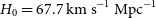


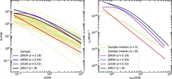


 Open access