


1. Introduction
The concept of a boundary layer (BL), which was introduced more than 100 years ago by Prandtl (Reference Prandtl1904), plays an important role in science and engineering and has made a profound impact in fluid physics, aerodynamics and applied mathematics (Anderson Reference Anderson2005). It also has a close connection to many engineering problems ranging from skin friction drag to mass and heat transfer near a solid surface (Schlichting & Gersten Reference Schlichting and Gersten2000; Ahlers, Grossmann & Lohse Reference Ahlers, Grossmann and Lohse2009; Chillà & Schumacher Reference Chillà and Schumacher2012). A BL flow is developed between a flat solid surface and the bulk fluid flow, because the fluid velocity at a stationary solid wall is zero under the no-slip boundary condition so that the viscous effect (and thus the velocity gradient) becomes significant in the region. Similarly, a thermal BL forms when a fluid moves along a heated (or cooled) solid wall. In this case, the molecular thermal diffusion (and hence the temperature gradient) becomes significant in the BL region.
The thermal BL in turbulent Rayleigh–Bénard convection (RBC) with Rayleigh number (dimensionless buoyancy)  $Ra\gtrsim 10^{8}$ is an example in which the BL is not fully turbulent but there are significant fluctuations resulting from intermittent eruptions of thermal plumes from the BL (Kadanoff Reference Kadanoff2001; Shishkina et al. Reference Shishkina, Horn, Wagner and Ching2015; Wang, He & Tong Reference Wang, He and Tong2016; Wang et al. Reference Wang, Lai, Song and Tong2018a). In the laboratory, RBC is realized in a confined fluid layer of height $H$, which is heated from below and cooled from above with a vertical temperature difference $\Delta T$ parallel to gravity. When $\Delta T$ (or $Ra$) is large enough, the bulk fluid becomes turbulent and heat is transported predominantly by convection. As a wall-bounded flow, RBC has temperature and velocity BLs adjacent to the conducting plates, and their dynamics are of great importance, as the thermal BLs determine the global heat transport of the system (Ahlers et al. Reference Ahlers, Grossmann and Lohse2009; Chillà & Schumacher Reference Chillà and Schumacher2012).
Compared with the large number of investigations of the BL dynamics near solid surfaces, our understanding of the BL flow near stable liquid interfaces is rather limited (Keulegan Reference Keulegan1944; Lock Reference Lock1951; Anderson, McFadden & Wheeler Reference Anderson, McFadden and Wheeler1998; Leal Reference Leal2007; Nepomnyashchy, Simanovskii & Legros Reference Nepomnyashchy, Simanovskii and Legros2012). This is partially caused by the fact that unlike inert and rigid solid surfaces, liquid interfaces are soft and dynamic and often involve complex transport processes and non-equilibrium fluctuations with a large number of fluid parameters, such as interfacial tension, fluid densities, viscosities and thermal conductivities. As a result, in many cases of interest, the boundary conditions at the liquid interface may not be specified a priori but have to be solved self-consistently with the bulk flow. Because high-resolution experimental characterization of the BL flow near a liquid interface is challenging and available experiment results are rare (Naumov, Skripkin & Shtern Reference Naumov, Skripkin and Shtern2021), our current understanding of the BL dynamics near a liquid interface relies mainly on the results from molecular dynamic simulations and numerical calculations (Sahraoui & Kaviany Reference Sahraoui and Kaviany1994; Padilla, Toxvaerd & Stecki Reference Padilla, Toxvaerd and Stecki1995; Stecki & Toxvaerd Reference Stecki and Toxvaerd1995; Chen, Jasnow & Viñals Reference Chen, Jasnow and Viñals2000; Koplik & Banavar Reference Koplik and Banavar2006; Hu, Zhang & Wang Reference Hu, Zhang and Wang2010; Razavi, Koplik & Kretzschmar Reference Razavi, Koplik and Kretzschmar2014; Vatin et al. Reference Vatin, Duvail, Guilbaud and Dufrêche2021).
These studies, however, were conducted under highly idealized conditions, such as a perfectly static liquid interface without any fluctuations, and reported a velocity slip (or jump) across the liquid interface. Direct measurement of the BL properties near a liquid interface is, therefore, needed in order to test different ideas. Understanding the BL flow near liquid interfaces is also relevant to a number of important natural phenomena, such as coupled ocean–atmosphere flows (Neelin, Latif & Jin Reference Neelin, Latif and Jin1994) and convection of the Earth's upper and lower mantles (Olson, Silver & Carlson Reference Olson, Silver and Carlson1990; Tackley Reference Tackley2000), and many industrial applications ranging from the liquid-encapsulated crystal growth technique (Prakash & Koster Reference Prakash and Koster1994) to solvent extraction (Holmberg, Shah & Schwuger Reference Holmberg, Shah and Schwuger2002).
In this work, we demonstrate that turbulent RBC in two stacking layers of immiscible fluids, as illustrated in figure 1(a), is an ideal quasi-two-dimensional (2-D) system for the study of the thermal BL dynamics near the liquid–liquid interface. The convective flow in each fluid layer is turbulent and possesses the key features of turbulent convection (Xie & Xia Reference Xie and Xia2013; Liu et al. Reference Liu, Chong, Wang, Ng, Verzicco and Lohse2021, Reference Liu, Chong, Yang, Verzicco and Lohse2022), which have been observed in single-layer convection (Song, Villermaux & Tong Reference Song, Villermaux and Tong2011; Wang et al. Reference Wang, He and Tong2016, Reference Wang, Lai, Song and Tong2018a; Wang, He & Tong Reference Wang, He and Tong2019; Wang et al. Reference Wang, Wei, Tong and He2022). A well-developed thermal BL is formed on each side of the liquid interface, which is stable and remains at an (average) position with minimal movement. Nevertheless, because of the coupling of the large-scale flows between the two immiscible fluid layers (Xie & Xia Reference Xie and Xia2013; Liu et al. Reference Liu, Chong, Wang, Ng, Verzicco and Lohse2021, Reference Liu, Chong, Yang, Verzicco and Lohse2022), the liquid interface undergoes strong BL fluctuations with a net convective heat flux passing through the interface. A central finding of this investigation is that the measured BL profiles near the liquid interface can be well described by the BL equations for a solid wall modified by a thermal slip length  $\ell _T$, which is directly linked to the convective heat flux passing through the liquid interface.

Figure 1. (a) Sketch of the experimental set-up for the measurement of local temperature profiles along the central vertical axis of the two-layer convection cell. The red arrows indicate the velocity components and spatial coordinates used in the experiment. (b) Sketch of a normalized temperature profile  $\theta (z)$ near a liquid interface with a thermal slip length $\ell _T$.
The remainder of the paper is organized as follows. We first describe the experimental and numerical methods in § 2. Experimental results are presented in § 3. Further theoretical analyses are given in § 4. Finally, the work is summarized in § 5.
2. Experimental and numerical methods
2.1. Experiment
As illustrated in figure 1(a), the two-layer convection experiment is conducted in a thin disk, whose cross-section has a stadium shape with a square of size  $D = 20$ cm sandwiched by two semicircles on the top and bottom sides. The cell's central axis is aligned vertically parallel to gravity, and the cell has an overall height $H=2D$, width $W=D$ and thickness $S=2$ cm. The top (and bottom) semicircular sidewall is made of 0.8 cm thick copper electroplated with a thin layer of nickel, and its temperature is controlled to an accuracy of 50 mK. Other walls of the cell are made of 1.8 cm thick transparent Plexiglas. The upper half of the cell is filled with (lighter) distilled water and the lower half of the cell is filled with a (heavier) fluorinated liquid, FC770 (3M Fluorinert FC770), which is immiscible with water. The bottom copper plate of the cell is heated using two silicon rubber film heaters, which are connected in parallel and sandwiched on the back side of the curved copper plate. The two film heaters provide a constant and uniform heat flux to the cell. The top copper plate is cooled by two counter-flowing water channels, in which cooling water is regulated by a temperature-controlled chiller (NESLAB, RTE740) with a temperature stability of 10 mK. Fine temperature control is achieved through an active feedback network using thermistors (model 4006, Omega) for real-time temperature measurement. The thermistors have an accuracy of 5 mK, and are embedded in each copper plate 1 mm away from the surface.
Compared with the upright cylindrical cells that are commonly used for the study of turbulent convection, the quasi-2-D thin-disk cell used in this experiment offers several unique features for the study of two-layer RBC attempted here. First, with each fluid occupying half of the cell, the cross-section of the half-cell has an aspect ratio of unity that accommodates the single-roll structure of the large-scale circulation (LSC) in each fluid layer. The corner flow is minimized by using two semicircular sidewalls, so that the LSC across the near-circular cross-section can have a steady rotation along a fixed orientation. Second, because the flow is confined in a thin disk, no three-dimensional (3-D) flow modes can be excited in this system. The quasi-2-D flow in the thin-disk cell, therefore, has a better geometry satisfying the assumption of the BL theory for a 2-D flow over an infinite horizontal plane. These simplifications allow us to have a stringent test of the theory.
In cylindrical cells, however, the large-scale flow has several 3-D flow modes, such as the torsional and sloshing modes (Brown & Ahlers Reference Brown and Ahlers2008, Reference Brown and Ahlers2009; Xi et al. Reference Xi, Zhou, Zhou, Chan and Xia2009; Ji & Brown Reference Ji and Brown2020), which may cause additional complications to the study of the LSC and BL dynamics. The strong coupling between the BL dynamics and complex 3-D large-scale flow in a closed cylinder, which has been studied in recent numerical simulations (van Reeuwijk, Jonker & Hanjalić Reference van Reeuwijk, Jonker and Hanjalić2008; Scheel, Kim & White Reference Scheel, Kim and White2012; Shi, Emran & Schumacher Reference Shi, Emran and Schumacher2012; Stevens et al. Reference Stevens, Zhou, Grossmann, Verzicco, Xia and Lohse2012; Wagner, Shishkina & Wagner Reference Wagner, Shishkina and Wagner2012; van der Poel, Stevens & Lohse Reference van der Poel, Stevens and Lohse2013; Shishkina, Horn & Wagner Reference Shishkina, Horn and Wagner2013; Scheel & Schumacher Reference Scheel and Schumacher2014), makes a quantitative comparison between experiment and 2-D BL theory difficult. Finally, the thin-disk cell allows us to conduct precise shadowgraph measurements to visualize the large-scale flow and plume emission dynamics near the liquid interface (see § 3.4 for further discussion). Similar thin-disk cells have been used in recent experiments to study the thermal BL profiles near a conducting plate (Wang et al. Reference Wang, He and Tong2016, Reference Wang, Lai, Song and Tong2018a), the LSC dynamics (Song et al. Reference Song, Villermaux and Tong2011, Reference Song, Brown, Hawkins and Tong2014; Wang et al. Reference Wang, Xu, He, Yik, Wang, Schumacher and Tong2018b) and the statistical properties of temperature fluctuations across a closed convection cell (Wang et al. Reference Wang, He and Tong2019, Reference Wang, Wei, Tong and He2022). This is a ‘simple but not simpler’ convection system, which possesses key features of turbulent convection and offers a natural platform for the study of the boundary conditions and BL dynamics at a stable liquid interface.
The two experimental control parameters in the convection experiment, the Rayleigh number  $Ra$ and the Prandtl number $Pr$, are defined as $Ra_i = \chi _i g D^3 \Delta T_i/(\nu _i\kappa _i)$ and $Pr_i = \nu _i/\kappa _i$, respectively, where the subscript $i$ is used to indicate the two different fluid layers with $i=LF$ for FC770 and $i=LW$ for water, $g$ is the gravitational acceleration and $\Delta T_i$ is the temperature difference across the $i$th fluid layer of height $D$. The values of the thermal expansion coefficient $\chi _i$, kinematic viscosity $\nu _i$ and thermal diffusivity
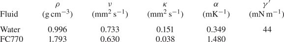
  $\kappa _i$ of each fluid are given in table 1. In the experiment, we vary the total temperature difference, $\Delta T=\Delta T_{LF}+\Delta T_{LW}$, across the cell, so that the resulting $Ra_{LF}$ is varied in the range $3.6 \times 10^{10} \lesssim Ra_{LF} \lesssim 1.8 \times 10^{11}$ and $Ra_{LW}$ is in the range $5.8 \times 10^{8} \lesssim Ra_{LW} \lesssim 6.8 \times 10^{8}$. The temperature of the bulk FC770 layer is kept at 30 $^\circ$C, so that $Pr_{LF}$ is fixed at 21.8. Under these experimental conditions, we find the interface between the two fluids is stable and remains at the (average) position $z=0$ with minimal movement. In this case, the two-layer system can be envisioned as two single-fluid subsystems, each having its own $Ra_i$ and $Pr_i$, and they are coupled dynamically through a stable liquid interface of surface tension $\gamma '\simeq 44\,{\rm mN}\,{\rm m}^{-1}$. This value of $\gamma '$ was obtained from a capillary force measurement using an atomic force microscope with a hanging glass fibre probe penetrating through an FC770–water interface at ambient temperature ${\sim }25^\circ$C (Guan et al. Reference Guan, Barraud, Charlaix and Tong2017; Guo et al. Reference Guo, Xu, Qian, Di, Doi and Tong2019). In this work, we focus on the two simultaneously measured thermal BLs in the FC770 fluid; one is near the upper liquid interface (LF) and the other is near the lower conducting plate (SF), where the subscripts $L$ and $S$ represent the liquid and solid, respectively.
Table 1. Two liquid samples used in the experiment and their literature values of density  $\rho$, dynamic viscosity $\mu$, thermal diffusivity $\kappa$, thermal conductivity $k$, thermal expansion coefficient $\chi$ and surface tension with air $\gamma$ (all at $30\,^\circ$C). The properties of water and FC770 are obtained, respectively, from Lide (Reference Lide2004) and 3MTM (2019).

To reduce the capillary effect at the liquid interface, two identical waterproof thermistors (AB6E3-B05KA202R, Thermometrics) with a diameter of 0.17 mm and a time constant of 10 ms are used to measure the local temperature of the convecting fluid. The two thermistors are assembled together with one bead pointing upward and the other bead pointing downward, as shown in figure 1(a). Thermistor 1 is used to measure the local temperature profile  $T(z)$ near the top cooling plate and the BL beneath the liquid interface. Thermistor 2 is used to measure the temperature profile $T(z)$ near the bottom heating plate and the BL above the liquid interface. These two thermistors are attached to a thin stainless steel tube that can move vertically along the central vertical axis of the cell. The tube is mounted on a translational stage, which is controlled by a stepping motor with a position resolution of 50 $\mathrm {\mu }$m. In the experiment, the entire convection cell is placed inside a thermostat box, whose temperature is maintained at the same temperature as the mean temperature of the bulk fluid of FC770 ( $30\,^{\circ }$C), in order to minimize heat exchange between the convecting fluid and the surroundings.
When the two thermistors move along the central axis of the cell, they measure the local temperature  $T(z,t)$ at an accuracy of 5 mK. From the measured time series, we obtain the normalized mean temperature profile:
 \begin{equation} \theta(z)\equiv \frac{|\langle T(z,t) \rangle_t-T_B|}{\varDelta_B}, \end{equation}
where  $\varDelta _B \equiv |T_B - T_0|$ is the temperature difference across the BL with $T_B$ being the interface temperature and $T_0$ being the bulk fluid (FC770) temperature. In the above, $\langle \cdots \rangle _t$ denotes an average over time $t$. Similarly, we obtain the temperature variance profile,
 \begin{equation} \eta(z) \equiv \langle [T(z,t)-\langle T(z,t)\rangle_t]^2\rangle_t, \end{equation}
near the liquid interface.
2.2. Direct numerical simulation (DNS)
The governing equations of the convective flow are the incompressible Navier–Stokes equations coupled with the convective heat equation under the Boussinesq approximation. The dimensionless form of these equations in each layer is given by
 \begin{gather} \widehat{\boldsymbol{\nabla}}\boldsymbol{\cdot} \hat{\boldsymbol u}=0, \end{gather}
 \begin{gather} \hat{\boldsymbol u}_{\hat t}+(\hat{\boldsymbol u}\boldsymbol{\cdot} \widehat{\boldsymbol{\nabla}})\hat{\boldsymbol u}={-}\frac{1}{\rho_i/\rho_0}\widehat{\boldsymbol{\nabla}}\hat p+\frac{1}{\sqrt{Ra_i/Pr_i}}\widehat{\boldsymbol{\nabla}}^2\hat{\boldsymbol u} +\frac{\alpha_i}{\alpha_0}\hat T\boldsymbol{e}_{\hat z}, \end{gather}
 \begin{gather} \hat T_{\hat t} +(\hat{\boldsymbol u}\boldsymbol{\cdot} \widehat{\boldsymbol{\nabla}})\hat T=\frac{1}{\sqrt{Ra_iPr_i}}\widehat{\boldsymbol{\nabla}}^2\hat T,\end{gather}
where the subscript  $i$ is used to indicate the two different fluid layers with $i = 0$ for the lower FC770 layer and $i = 1$ for the upper water layer. The dimensionless parameters $Ra_i$, $Pr_i$ and Weber number $We$ to be used below are defined as
 \begin{equation} \left. \begin{aligned} & Ra_i = \frac{g\alpha_0\Delta T D^3}{\nu_i\kappa_i}, \\ & Pr_i = \frac{\nu_i}{\kappa_i},\\ & We = \frac{\rho_0 g\alpha_0 \Delta T D^2}{\gamma'}. \end{aligned} \right\} \end{equation}
The length, time, velocity, pressure and temperature are made dimensionless by the half-height of the cell  $D$, the free-fall time $T_f = \sqrt {D/(g\alpha _0\Delta T)}$, the free-fall velocity $U_f = \sqrt {g\alpha _0\Delta T D}$, the free-fall pressure $p_f = \rho _0g\alpha _0 \Delta T D$ and the temperature difference $\Delta T$ across the whole cell, respectively. Note that the definition of $Ra_i$, $Pr_i$ and $We$ in (2.6) is different from that used in the experiment, as mentioned above.
The dimensionless boundary conditions at the cell wall are given by
 \begin{equation} \left. \begin{aligned}
& \hat{\boldsymbol u}|_{{{all\ solid\ walls}}}=0,\\ &
\boldsymbol n\boldsymbol{\cdot}
\widehat{\boldsymbol{\nabla}}\hat T|_{{{all\
non\text{-}conducting\ walls}}}=0,\\ & \hat T|_{{{lower\
conducting\ wall}}}=0.5,\\ & \hat T|_{{{upper\ conducting\
wall}}}={-}0.5. \end{aligned} \right\}
\end{equation}
\begin{equation} \left. \begin{aligned}
& \hat{\boldsymbol u}|_{{{all\ solid\ walls}}}=0,\\ &
\boldsymbol n\boldsymbol{\cdot}
\widehat{\boldsymbol{\nabla}}\hat T|_{{{all\
non\text{-}conducting\ walls}}}=0,\\ & \hat T|_{{{lower\
conducting\ wall}}}=0.5,\\ & \hat T|_{{{upper\ conducting\
wall}}}={-}0.5. \end{aligned} \right\}
\end{equation}
Here the subscript ‘all solid walls’ refers to all solid boundaries of the convection cell, ‘lower conducting wall’ refers to the bottom heating plate of the cell, ‘upper conducting wall’ refers to the top cooling plate of the cell and ‘all non-conducting walls’ refers to all solid boundaries of the cell except the bottom heating plate and top cooling plate.
The governing equations are solved numerically using the open-source code Nek5000 (Fischer Reference Fischer1997), which uses a spectral element method to accurately resolve the gradients in the velocity field  $\hat {\boldsymbol u}(\boldsymbol r,t)$ and temperature field $\hat T(\boldsymbol r, t)$. In the simulation, the time-derivative terms are discretized by the backward differentiation formula, the nonlinear convective terms are treated explicitly and the linear diffusive terms are approximated implicitly. This scheme leads to a Poisson equation for pressure and Helmholtz equations for the velocity components and temperature. These equations are written in a weak formulation and discretized by the Galerkin method using the $N$th-order Lagrangian interpolation polynomials as the basis functions on Gauss–Lobatto–Legendre (GLL) collocation points (Deville, Fischer & Mund Reference Deville, Fischer and Mund2002). More details about the numerical scheme and mesh resolution requirements can be found in Fischer (Reference Fischer1997), Deville et al. (Reference Deville, Fischer and Mund2002) and Scheel, Emran & Schumacher (Reference Scheel, Emran and Schumacher2013). All the gradients in the post-numerical processing are also calculated on the GLL collocation points with spectral accuracy.
Nek5000 models the liquid interface between two immiscible fluids using the arbitrary Lagrangian–Eulerian moving mesh approach (Ho Reference Ho1989). In the simulation, we specified the material properties in each fluid layer according to (2.5)–(2.6) and table 2. The liquid interface is tracked by a moving computational mesh. During the simulation, at each time step, the mesh near the interface moves together with the interface because of the flow inertia. The deformed (curved) interfacial mesh generates an interfacial tension, which resists the deformation. This resistive force acts on both sides of the fluid as an external force via the momentum equations. The velocity across the interface is assumed continuous. The pressure jump across the interface is balanced by the surface tension and the jump of the normal viscous stresses. The temperature across the interface is assumed continuous based on the experimental observations. The dimensionless jump conditions of the flow variables across the liquid interface are given by
 \begin{equation} \left. \begin{aligned} & [\hat u]=0,\\ & [\hat p]={-}\frac{1}{We}\hat K+[\hat \tau_n],\\ & [\hat T]=0, \end{aligned} \right\} \end{equation}
where  $[\,\cdot\,]$ denotes the jump of a flow variable across the interface, $\hat K$ is the dimensionless curvature of the interface and $\hat \tau _n$ is the dimensionless normal viscous stress on the interface.
Table 2. Material properties of FC770 and water used in the simulation. The temperature difference  $\Delta T$ across the cell is set at $\Delta T =11.5\,\textrm {K}$ and the half-height of the cell is $D = 20$ cm. The interfacial tension of the water–FC770 interface is estimated as $\gamma '\simeq 44\,\textrm {mN}\,\textrm {m}^{-1}$. The corresponding dimensionless parameters defined in (2.6) are: $Ra_0 = (g\alpha _0\Delta T D^3)/(\nu _0\kappa _0) \simeq 6.4\times 10^{10}$, $Pr_0 = \nu _0/\kappa _0 \simeq 18.46$, $Ra_1 = (g\alpha _0\Delta T D^3)/(\nu _1\kappa _1) \simeq 1.2\times 10^{10}$, $Pr_1 = \nu _1/\kappa _1 \simeq 4.86$ and $We = (\rho _0 g\alpha _0 \Delta T D^2)/\gamma '\simeq 300$.
Since the local  $Ra_i$ in the lower FC770 layer and upper water layer, as defined in the experiment, is in the range $10^8$– $10^{10}$, we design the computational mesh of the DNS accordingly. The finally realized local dimensionless parameters in the simulation are: $Ra_{LF}= g\alpha _0\Delta T_0 D^3/(\nu _0\kappa _0)\simeq 3.2\times 10^{10}$, $Pr_{LF} = \nu _0/\kappa _0\simeq 18.46$, $Ra_{LW} = g\alpha _1\Delta T_1 D^3/(\nu _1\kappa _1)\simeq 1.4\times 10^{9}$, $Pr_{LW}\simeq 4.86$ and $We_{LF}=\rho _0g\alpha _0\Delta T^2_0/\gamma '\simeq 150$. In a recent DNS study of thermal BL dynamics in a single fluid layer (Wang et al. Reference Wang, Lai, Song and Tong2018a), the smallest primary mesh size near the solid boundary was set as $3.87 \times 10^{-3}D$, which is approximately the thermal BL thickness $\lambda$ measured in the experiment. The polynomial order within each mesh element was set to $N =7$ so that one has eight grid points to resolve the thermal BLs with the smallest secondary mesh size of $2.61 \times 10^{-4}D$. This mesh size was tested to be sufficient for the $Ra$ range between $10^9$ and $10^{10}$ in the thin-disk convection cell. The obtained thermal BL profiles from the DNS were found to be in good agreement with the experiment (Wang et al. Reference Wang, Lai, Song and Tong2018a). With a similar DNS accuracy, we set the smallest primary mesh size near the solid boundary to $4.1 \times 10^{-3}D$ in the current study. This mesh size should be sufficient for the current simulation, as the Prandtl number $Pr_{LF}$ in the lower FC770 layer is approximately 3.8 times larger than that in the upper water layer. In addition, we set the smallest primary mesh size near the liquid interface to $4.4 \times 10^{-3}D$ in the current study, which is only ${\sim }7\,\%$ larger than that near the solid boundary. As is shown below, the measured mean temperature gradient near the liquid interface is approximately 2.5 times smaller than that near the solid conducting plates. Therefore, the primary mesh size used for the liquid interface is sufficient to resolve the thermal BL variations near the interface. Figure 2 shows the primary computational mesh used in the simulation. We set the polynomial order to $N = 7$ so that we have $8^3 = 512$ grid points within each primary element. Based on the GLL collocation, the smallest secondary mesh size at the liquid interface is $2.83 \times 10^{-4}D$.

Figure 2. Primary computational mesh used in the simulation. There are a total of 6300 primary elements on the vertical cross-section and 6 primary elements across the thickness direction. For each primary element, there are  $8 \times 8 \times 8$ secondary nodes with polynomial order of 7.
The time step is set at  $4 \times 10^{-5}T_f$ such that the motion of the interface can be resolved well using the moving mesh grid. We run the simulation for $50T_f$ to reach the steady state, followed by a continuous running for at least another $100T_f$ to collect data for statistical analysis. The instantaneous flow fields with a moving mesh are interpolated to a fixed mesh with the same configuration as the initial one for further post-numerical processing. The vertical profile of the local properties is computed along a thin column surrounding the vertical $z$ axis of the cell with $x = y = 0$ and is averaged over the cross-section of the thin column with a small area of $0.01D^2$.
3. Experimental results
3.1. Temperature measurements near the liquid interface
Unlike the temperature of the top and bottom plates, which is directly controlled in the experiment, the temperature at the liquid interface is a dynamic response of the convection system. While the vertical position of the liquid interface remains stable on average, it fluctuates with time due to the convective heat transport across the liquid interface. Figure 3(a) shows the measured mean temperature profile  $\langle T(z,t)\rangle _t$ across the liquid interface. The mean temperature profiles show hysteresis near the liquid interface. This is caused by the wetting effect of the liquid interface to the thermistor tip, which stretches the interface when the thermistor tip passes through it. The black circles measured by Thermistor 1 when it moves upwards before touching the interface from below (FC770 side, $z<0$) do not suffer this interface stretching effect. Similarly, the red triangles measured by Thermistor 2 when it moves downwards before touching the interface from above (water side, $z>0$) do not suffer the interfacial wetting either. We, therefore, use the linear extrapolation of the local slope of the measured $\langle T(z,t)\rangle _t$ on both sides of the liquid interface (coloured solid lines in figure 3a) to determine the intercept location, which is defined as the interface location, as shown by the vertical dotted line in figure 3(a). The experimental uncertainty for the interface location determined by the linear extrapolation is ${\pm }50\,\mathrm {\mu }$m (one data point on either side of the interface). Figure 3(b) shows the final mean temperature profile $\langle T(z,t)\rangle _t$ across the liquid interface.

Figure 3. (a) Measured mean temperature profile  $\langle T(z,t)\rangle _t$ across the liquid interface. The black circles are obtained with Thermistor 1 (see inset) moving upwards across the interface from below and the red triangles are obtained with Thermistor 2 moving downwards across the interface from above. The measurements are made at $Ra_{LF} = 1.8 \times 10^{11}$ and $Ra_{LW}= 6.8 \times 10^8$. The coloured solid lines indicate the local slope of $\langle T(z,t)\rangle _t$ near the liquid interface. The vertical dotted line indicates the (extrapolated) location of the liquid interface. Inset shows the assembly of the two thermistors, which can move vertically along the central axis of the convection cell (black double-headed arrow). (b) Replot of the final mean temperature profile $\langle T (z,t)\rangle _t$ across the liquid interface with black circles on the FC770 side ( $z<0$) and red triangles on the water side ( $z >0$). The coloured solid lines indicate the local slope of $\langle T (z,t)\rangle _t$ near the liquid interface. The resulting thermal BL thickness on the FC770 side is $\lambda _{LF}=1.07$ mm and that on the water side is $\lambda _{LW}=1.35$ mm.
As shown in figure 3(b), the time-averaged temperature profile  $\langle T(z,t)\rangle _t$ across the liquid interface is continuous (within the experimental resolution) but its slope has a finite jump across the interface, as indicated by the two solid lines with slopes of $-11.7\,\textrm {K}\,\textrm {mm}^{-1}$ (on the FC770 side) and $-3.6\,\textrm {K}\,\textrm {mm}^{-1}$ (on the water side), respectively. The ratio of the two slopes, $11.7/3.6\simeq 3.25$, is smaller than the thermal conductivity ratio, $k_{LW}/k_{LF}=9.8$, indicating that the heat flux across the liquid interface involves both the conduction ( $-k(\textrm {d}\langle T(z,t)\rangle _t/\textrm {d}z)$) and convection ( $\rho C_p\langle w^\prime T^\prime \rangle$) contributions (see § 3.4 for further discussion). Here $k$,
$k$,  $\rho$ and $C_p$ are, respectively, the thermal conductivity, density and specific heat of the convecting fluid, and $\langle w^\prime T^\prime \rangle$ is the velocity–temperature correlation function with $T^\prime$ and $w^\prime$ being, respectively, the local temperature and vertical velocity fluctuations. The measured $\langle T(z,t)\rangle _t$ reveals a well-developed thermal BL formed on each side of the liquid interface, whose thickness $\lambda$ is defined as the distance at which the linear extrapolation of the mean temperature gradient at the interface intersects the bulk fluid temperature (Wang et al. Reference Wang, He and Tong2016), as marked in figure 3(b).
Figure 4 shows the measured temperature variance profile  $\eta _{LF}(\delta z)$ across the liquid interface, which shows hysteresis similar to that shown in figure 3(a). The black circles measured by Thermistor 1 when it moves upwards before touching the interface from below (FC770 side, $z<0$) do not suffer the wetting effect of the thermistor. Similarly, the red triangles measured by Thermistor 2 when it moves downwards before touching the interface from above (water side, $z>0$) do not suffer the interfacial wetting either. The measured temperature variance profile $\eta _{LF}(\delta z)$ is a direct measure of BL fluctuations and is absent in laminar BLs. The measured $\eta _{LF}(\delta z)$ has a sharp peak on each side of the interface and the peak height on the FC770 side ( $z<0$) is much larger than that on the water side ( $z>0$). This peak is caused by the intermittent emission of thermal plumes from the shoulder of the thermal BLs (Wang et al. Reference Wang, He and Tong2016, Reference Wang, Lai, Song and Tong2018a).

Figure 4. Measured temperature variance profile  $\eta (z)$ across the liquid interface. The black circles are obtained with Thermistor 1 (see inset) moving upwards across the interface from below and the red triangles are obtained with Thermistor 2 moving downwards across the interface from above. The measurements are made at $Ra_{LF} = 1.8 \times 10^{11}$ and $Ra_{LW}= 6.8 \times 10^8$. The vertical dotted line indicates the (extrapolated) location of the liquid interface, as determined in figure 3(a).
3.2. Normalized mean temperature profiles near the lower conducting plate and near the liquid interface
Figure 5(a) shows the normalized mean temperature profiles  $\theta _{SF}(\delta z)$ obtained at different values of $Ra_{LF}$ near the bottom heating plate. Here $\delta z$ is used to indicate the distance away from the solid interface. It is seen that all the normalized mean temperature profiles collapse onto a single master curve, once $\delta z$ is normalized by the BL thickness $\lambda _{SF}$. The measured $\theta _{SF}(\delta z)$ thus has a universal form independent of $Ra_{LF}$. Similar results were also obtained in previous studies (Wang et al. Reference Wang, He and Tong2016). The three sets of data are well described by the following equation (Shishkina et al. Reference Shishkina, Horn, Wagner and Ching2015):
 \begin{equation} \theta_{SF}(\xi;c)=\int_0^{\xi}\left(1+\frac{\kappa_t(\epsilon)}{\kappa}\right)^{{-}c}\,{\mathrm{d}} \epsilon\simeq\int_0^{\xi}(1+a\epsilon^3)^{{-}c}\,{\mathrm{d}} \epsilon, \end{equation}
where  $\xi =\delta z/\lambda _{LF}$ and $\kappa$ is the molecular thermal diffusivity. To derive the second equality of (3.1), Shishkina et al. (Reference Shishkina, Horn, Wagner and Ching2015) introduced the turbulent diffusivity $\kappa _t(\delta z)$ to describe the convective heat transfer, $\langle w^\prime T^\prime \rangle =-\kappa _t(\delta z)\partial _zT$, and showed that $\kappa _t(\delta z)$ near a solid wall has a scaling form, $(\kappa _t(\delta z)/\kappa )_{SF} \simeq a\xi ^3$, where $a$ is a proportionality constant. The exponent $c$ (
$c$ ( $\geq 1$) is a fitting parameter, which is related to $a$ via the condition $a = [\varGamma (1/3)\varGamma (c-1/3)/(3\varGamma (c))]^3$. The best fit to (3.1) is obtained with $c=1.55$ ( $a\simeq 0.918$), which is shown in figure 5(a) (solid line). When $c \to \infty$ ( $a \to 0$), $\theta _{SF}(\xi ;c)$ approaches the Prandtl–Blasius–Pohlhausen form (Landau & Lifshitz Reference Landau and Lifshitz1987) for laminar BLs without fluctuations (dotted line). The lower bound for the value of $c$ is $c=1$ (dashed line).

Figure 5. (a) Normalized mean temperature profiles  $\theta _{SF}(\delta z)$ as a function of the normalized distance $\delta z/\lambda _{SF}$ away from the bottom conducting plate for different values of $Ra_{LF}$. The error bars show the standard deviation of the black circles. The solid line shows a fit of (3.1) to the data points with $c=1.55$. The dotted and dashed lines are the calculated $\theta _{SF}(\xi ;c)$ using (3.1) with $c=\infty$ and $c=1$, respectively. (b) Normalized mean temperature profile $\theta _{LF}(\delta z)$ as a function of the normalized distance $\delta z/\lambda _{LF}$ away from the liquid interface for different values of $Ra_{LF}$. The error bars show the standard deviation of the black circles. The dotted and dashed lines are, respectively, the calculated $\theta _{SF}(\xi ;c)$ using (3.1) with $c=\infty$ and $c=1.55$. The solid line shows a fit of (4.4) to all the data points with $c=1.55$ and $\xi _0=0.23$.
Figure 5(b) shows the normalized mean temperature profile  $\theta _{LF}(\delta z)$ near the liquid interface on the FC770 side. Here $\delta z$ is used to indicate the distance away from the liquid interface. Similar to $\theta _{SF}(\delta z)$, all the normalized mean temperature profiles $\theta _{LF}(\delta z)$ obtained at different values of $Ra_{LF}$ have a $Ra_{LF}$-invariant form, once $\delta z$ is normalized by the BL thickness $\lambda _{LF}$. However, the actual shape of the measured $\theta _{LF}(\delta z)$ near the liquid interface shows considerable deviations from the measured $\theta _{SF}(\delta z)$ near the solid wall (dashed line with $c = 1.55$) and (3.1) is no longer able to fit the measured $\theta _{LF}(\delta z)$ directly with any value of $c \geq 1$.
3.3. Normalized temperature variance profiles near the lower conducting plate and near the liquid interface
Figure 6 shows a comparison between the measured  $\eta _{LF}(\delta z)$ near the liquid interface and $\eta _{SF}(\delta z)$ near the lower conducting plate. In the plot, $\eta _{LF}(\delta z)$ ( $\eta _{SF}(\delta z)$) is normalized by its peak value $\eta _0$ and $\delta z$ is normalized by $\lambda _{LF}$ ( $\lambda _{SF}$). All the normalized plots of $(\eta (\delta z)/\eta _0)_{LF}$ ( $(\eta (\delta z)/\eta _0)_{SF}$) for different values of $Ra_{LF}$ collapse onto a single master curve, indicating that the measured $(\eta (\delta z)/\eta _0)_{LF}$ ( $(\eta (\delta z)/\eta _0)_{SF}$) has a scaling form independent of $Ra_{LF}$.

Figure 6. (a) Normalized temperature variance profiles  $(\eta (\delta z)/\eta _0)_{LF}$ as a function of $\delta z/\lambda _{LF}$ away from the liquid interface for different values of $Ra_{LF}$. The solid line shows the calculated $\varOmega _{LF}(\xi ;\xi _0)$ using (4.8) with all the parameters already determined in (b) and figure 5. (b) Normalized plots of $(\eta (\delta z)/\eta _0)_{SF}$ as a function of $\delta z/\lambda _{SF}$ away from the lower conducting plate for different values of $Ra_{LF}$. The solid line shows the calculated $\varOmega _{SF}(\xi ;c,\varDelta _B^2/\eta _0,d,\alpha )$ with $c=1.55$, $\varDelta _B^2/\eta _0=128$, $d =5.3$ and $\alpha = 7.8$. The error bars show the experimental uncertainties of the black circles.
Recently, Wang et al. (Reference Wang, He and Tong2016) derived a BL equation for  $\varOmega _{SF}(\delta z)\equiv (\eta (\delta z)/\eta _0)_{SF}$ with $Pr > 1$:
 $$\begin{gather} (1+d\xi^3)\frac{{\mathrm{d}}^2\varOmega_{SF}(\xi)}{{\mathrm{d}}\xi^2}+(\beta+3d)\xi^2\frac{{\mathrm{d}}\varOmega_{SF}(\xi)}{{\mathrm{d}}\xi} +2\frac{\varDelta_b^2}{\eta_0}\frac{a\xi^3}{(1+a\xi)^{2c}}\nonumber\\ -\frac{1}{2} \frac{[{\mathrm{d}} \varOmega_{SF}(\xi)/{\mathrm{d}} \xi]^2}{\varOmega_{SF}(\xi)}-2\alpha\varOmega_{SF}(\xi)=0, \end{gather}$$
where  $\xi =\delta z/\lambda _{LF}$ and $a$ is given in (3.1). Equation (3.2) is an ordinary differential equation, which can be numerically solved using the Runge–Kutta method under the initial conditions
 \begin{equation} \varOmega_{SF}(\xi_p)=1,\quad \frac{\mathrm{d}\varOmega_{SF}(\xi_p)}{\mathrm{d}\xi}=0, \end{equation}
where  $\xi _p$ is the peak position of $\varOmega _{SF}(\xi )$, as shown in figure 6(b). The final solution $\varOmega _{SF}(\xi ;c,\varDelta _B^2/\eta _0,d,\alpha )$ has four parameters. The parameter $c$ (
$c$ ( $= 1.55$) has been obtained separately from the fitting of (3.1) to the measured $\theta _{SF}(\delta z)$, as shown in figure 5(a). The parameter $\delta ^2_B/\eta _0$ is a measurable quantity, which is directly determined from the experiment. There are only two adjustable parameters remaining, $d$ and $\alpha$, which are used to best fit the measured $(\eta (\delta z)/\eta _0)_{SF}$. As shown in figure 6(b), the measured $(\eta (\delta z)/\eta _0)_{SF}$ near the lower conducting plate is well described by (3.2) (black solid line).
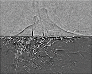
3.4. Visualization of thermal plumes near the liquid interface
In addition to the above time-averaged measurements of the temperature field across the liquid interface, we also use a shadowgraph technique (Settles Reference Settles2001) to visualize the instantaneous convective flow near the liquid interface. Details about the shadowgraph set-up are given in the Appendix. The shadowgraphic supplementary movie 1 available at https://doi.org/10.1017/jfm.2022.846 shows the emission dynamics of thermal plumes at the water–FC770 interface. It is found that cold plumes emit from the lower BL of the liquid interface and fall into the lower FC770 layer. Warm plumes, on the other hand, emit from the upper BL of the liquid interface and rise to the upper water layer. As a result, the liquid interface undergoes strong BL fluctuations with a net heat flux across the interface. Nevertheless, the liquid interface is stable and remains at an (average) position with minimal movement. From the zoom-in images of the shadowgraphic movie taken near the liquid interface, we find that shape fluctuations of the interface are at the level of 1 pixel, which corresponds to 0.1 mm for the imaging set-up used in the experiment.
Note that the boundary conditions at a liquid interface are very different from those at a solid wall. For a solid wall, both the mean velocity  $\langle w\rangle$ and velocity fluctuations $w^\prime$ (in the normal direction) are zero because of the no-slip boundary condition. For a stable liquid interface, however, we have $\langle w\rangle =0$ but $w^\prime \not =0$. In this case, the total heat flux $\varPhi$ across the liquid interface contains both the conduction and convection contributions, i.e. $\varPhi = -k(\textrm {d}\langle T(z,t)\rangle _t/\textrm {d}z) + \rho C_p\langle w^\prime T^\prime \rangle$. At the liquid interface, both $w^\prime$ and $T^\prime$ are non-zero. At the solid wall, however, we have $\langle w^\prime T^\prime \rangle =0$, and thus conduction becomes the dominant term in the BL. Hereafter, we discuss the effects of the non-zero $w^\prime$ and $T^\prime$ on the measured mean temperature profile and temperature variance profile near the liquid interface.
4. Further theoretical analysis
By a careful comparison between figures 6(a) and 6(b), we find that the measured  $\eta _{LF}(\delta z)$ near the liquid interface has a shape similar to that of $\eta _{SF}(\delta z)$ near the solid surface, except that the entire curve of $\eta _{LF}(\delta z)$ is shifted towards the origin by a small distance $\xi _0$ so that the measured $\eta _{LF}(\delta z)$ at the origin (i.e. at the interface) has a non-zero value and its peak position is shifted from $0.78\delta z/\lambda _{SF}$ to $0.63\delta z/\lambda _{LF}$. This finding suggests that the BL profiles near a liquid interface may be described by the BL equations for a solid wall modified by a slip length $\ell _T$, as illustrated in figure 1(b).
The mean temperature profile near the liquid interface can be described based on a truncated temperature profile  $\theta ^T_{SF}(\xi ;c,\xi _0)$ near the lower conducting plate with $\xi$ being equal to or larger than the slip length $\xi _0$. The truncated profile $\theta ^T_{SF}(\xi ;c,\xi _0)$ is the portion of the black curve in the blue coordinates { $\theta _{LF}(\delta z)$, $\delta z/\lambda _{LF}$}, as shown in figure 7, and has the form
 \begin{align} \theta^T_{SF}(\xi;c,\xi_0) &= \theta_{SF}(\xi+\xi_0;c)-\theta_{SF}(\xi_0;c)\nonumber\\ &= \int_0^{\xi+\xi_0}(1+a\xi^3)^{{-}c}\,{\mathrm{d}} \epsilon-\int_0^{\xi_0}(1+a\xi^3)^{{-}c}\,{\mathrm{d}} \epsilon\nonumber\\ &=\int_{\xi_0}^{\xi+\xi_0}(1+a\xi^3)^{{-}c}\,{\mathrm{d}} \epsilon = \int_0^{\xi}[1+a(\epsilon+\xi_0)^3]^{{-}c}\,{\mathrm{d}} \epsilon. \end{align}
The profile  $\theta ^T_{SF}(\xi ;c,\xi _0)$ has the following boundary conditions:
 \begin{equation} \theta^T_{SF}(\infty;c,\xi_0)= 1-\theta_{SF}(\xi_0;c) \end{equation}
and
 \begin{equation} \left.\frac{{\mathrm{d}} \theta^T_{SF}(\xi;c,\xi_0)}{{\mathrm{d}} \xi }\right|_{\xi=\xi_0} = (1+a\xi_0^3)^{{-}c}. \end{equation}
Figure 7. A sketch illustrating the two coordinate systems used to describe the mean temperature profiles near the lower conducting plate (black coordinates  $\{\theta _{SF}(\delta z), \delta z/\lambda _{SF}\}$) and near the liquid interface (blue coordinates { $\theta _{LF}(\delta z)$, $\delta z/\lambda _{LF}$}). The origin of the blue coordinates is shifted by an amount of { $\theta _{SF}(\xi _0;c)$, $\xi _0$} relative to that of the black coordinates. The black solid line shows the normalized mean temperature profile $\theta _{SF}(\xi ;c)$ in (3.1). The blue solid line shows the normalized mean temperature profile $\theta _{LF}(\xi ;c,\xi _0)$ in (4.4).
The normalized mean temperature profile  $\theta _{LF}(\xi ;c,\xi _0)$ near the liquid interface then takes the form
 \begin{equation} \theta_{LF}(\xi;c,\xi_0)=\frac{1}{1-\theta_{SF}(\xi_0;c)}\int_{0}^{b\xi}[1+ a(\epsilon+\xi_0)^3]^{{-}c}\,{\mathrm{d}} \epsilon, \end{equation}
where
 \begin{equation} b = \frac{1-\theta_{SF}(\xi_0;c)}{(1+a\xi_0^3)^{{-}c}}. \end{equation}
In the above, the prefactor  $[1-\theta _{SF}(\xi _0;c)]^{-1}$ is introduced to renormalize the slip-induced amplitude change of the temperature profile. Similarly, $b$ is used to renormalize the slip-induced local slope change of the temperature profile. This is equivalent to a correction of the BL thickness $\lambda _{LF}^\prime =\lambda _{LF}/b$ due to a slip. For small values of $\xi _0$, we have $b\simeq 1-\theta _{SF}(\xi _0;c)\simeq 1-\xi _0$, and thus the slip length $\ell _T \simeq \xi _0\lambda _{LF}/(1-\xi _0)$.
Equation (4.4) is shown by the blue curve in figure 7. It is seen that  $\theta _{LF}(\xi ;c,\xi _0)$ satisfies the normalized boundary conditions:
 \begin{equation} \theta_{LF}(\infty;c,\xi_0)= 1 \end{equation}
and
 \begin{equation} \left.\frac{{\mathrm{d}} \theta_{LF}(\xi;c,\xi_0)}{{\mathrm{d}} \xi }\right|_{\xi=0} =1, \end{equation}
as required by the definition of the normalized mean temperature profile. Equation (4.4) has two parameters. The parameter  $c$ (
$c$ ( $= 1.55$) has been obtained separately from the fitting of (3.1) to the measured $\theta _{SF}(\delta z)$ near the lower conducting plate, as shown in figure 5(a). The slip length $\xi _0$ is the only fitting parameter to be determined from the measured $\theta _{LF}(\xi ;c,\xi _0)$ near the liquid interface. The solid line in figure 5(b) shows a good fit of (4.4) to the experimental data with $\xi _0=0.23\pm 0.05$.
By the same considerations of the slip boundary condition, we find that the normalized temperature variance profile near the liquid interface takes the form
 \begin{equation} \varOmega_{LF}(\xi;\xi_0)=\varOmega_{SF}(b\xi+\xi_0;c,\varDelta_B^2/\eta_0,d,\alpha), \end{equation}
where  $b$ is used for rescaling of the BL thickness, $\lambda _{LF}^\prime =\lambda _{LF}/b$, owing to a slip at the liquid interface. The solid line in figure 6(a) shows the calculated $\varOmega _{LF}(\xi ;\xi _0)$ using (4.8) with no adjustable parameter; all of the parameters of $c=1.55$, $\xi _0=0.23$, $\varDelta ^2/\eta _0=128$, $d =5.3$ and $\alpha = 7.8$ used in the calculation are already determined in figures 5 and 6(b). An excellent agreement between the theory and experiment is obtained.
By comparing (4.4) with the first equality of (3.1), we find that the turbulent thermal diffusivity  $\kappa _t(\delta z)$ near a liquid interface should have a scaling form, $(\kappa _t(\xi )/\kappa )_{LF} = a(\xi +\xi _0)^3$. As $\kappa _t(\xi )$ is not a directly measurable quantity, we conduct DNS of two-layer RBC using the open-source code Nek5000 to test this prediction. The DNS is carried out at fixed values of $Ra_{LF}$, $Pr_{LF}$ and Weber number $We_{LF}$ (with interfacial tension $\gamma ' = 44\,\textrm {mN}\,\textrm {m}^{-1}$) in a vertical stadium-shaped thin disk having the same dimensions as those used in the experiment. While the resulting values of $Ra_{LF}$, $Pr_{LF}$ and $We_{LF}$ are not exactly the same as those in the experiment, they are nevertheless in the same parameter range as in the experiment. As shown in figure 8, the numerically calculated $(\kappa _t(\xi )/\kappa )_{LF}$ indeed has the expected power-law form with a slip length, $\xi _0=0.22\pm 0.02$, very close to the experimental value. Figure 8 thus further confirms that the slip length $\xi _0$ is indeed caused by the velocity and temperature fluctuations at the liquid interface.

Figure 8. Log–log plot of the numerically calculated turbulent thermal diffusivity profile  $(\kappa _t(\delta z)/\kappa )_{LF}$ as a function of $\delta z/\lambda _{LF}$ at $Ra_{LF} = 3.2 \times 10^{10}$, $Pr_{LF} = 18.46$ and Weber number $We_{LF}\simeq 150$. The solid line shows the power-law fit, $(\kappa _t(\delta z)/\kappa )_{LF} = 0.6(\delta z/\lambda _{LF}+\xi _0)^3$, in the region $\delta z/\lambda _{LF}\lesssim 4$ with $\xi _0=0.22$.
5. Conclusion
This work concerns a fundamental issue in interfacial dynamics, namely the boundary conditions at a stable liquid–liquid interface. The hydrodynamic boundary condition, which complements the Navier–Stokes equation, serves as a pillar of continuum hydrodynamics. Unlike other partial differential equations in physics, such as Maxwell's equations, for which the boundary conditions can be derived analytically from the equations themselves, the hydrodynamic boundary condition near a solid wall, which has been regarded as non-slip for more than a century (i.e. there is no relative motion at the liquid–solid interface), has never been derived from first principles. For this reason, the past decade has witnessed a surge of experimental and theoretical studies of the hydrodynamic boundary conditions at various liquid–solid interfaces (Lauga, Brenner & Stone Reference Lauga, Brenner and Stone2007). Compared with the large number of investigations of the BL dynamics near solid surfaces, our understanding of the BL flow near stable liquid interfaces is rather limited. Unlike inert and rigid solid surfaces, liquid interfaces are soft and dynamic and often involve complex transport processes and non-equilibrium fluctuations with a large number of fluid parameters. Because high-resolution experimental characterization of the BL flow near a liquid interface is challenging and available experiment results are rare, our current understanding of the BL dynamics near a liquid interface relies mainly on the results from molecular dynamic simulations and numerical calculations.
In this work, we demonstrate that quasi-2-D RBC in two stacking layers of immiscible fluids is a valuable experimental framework for the study of the boundary conditions at a stable liquid interface. Conceptually, this is a simple convection system with a constant heat flux provided by the lower heating plate, which has to go through the liquid interface and reaches the upper cooling plate (similar to a constant electric current going through two resistors connected in series). Because of the mismatch of the thermal properties between the two fluids, the temperature profile across the liquid interface forms a well-developed thermal BL on each side of the interface, instead of having a finite temperature jump. The two BLs are unstable, however, and emit thermal plumes on each side of the interface. From a careful flow visualization of the emission dynamics of thermal plumes at the water–FC770 interface, we find that cold plumes emit from the lower BL of the liquid interface, which fall into the lower FC770 layer. Warm plumes, on the other hand, emit from the upper BL of the liquid interface and rise to the upper water layer. As a result, the liquid interface undergoes strong BL fluctuations and heat transport is realized with a net heat flux across the interface without involving macroscopic mass transport of the immiscible fluid molecules.
With this experimental framework, we are able to find a quantitative relation between BL fluctuations and the thermal slip length  $\ell _T$ of the BL profiles. The measured mean temperature and temperature variance profiles near the liquid interface are found to be well described by the BL equations for a solid wall, so long as a thermal slip length $\ell _T$ is included to account for the convective heat flux passing through the liquid interface. For a solid wall, the no-slip (and no-fluctuation) boundary conditions (i.e. $\langle w^\prime T^\prime \rangle =0$) dictate that the turbulent thermal diffusivity goes as $\kappa _t(\xi )/\kappa \sim \xi ^3$ in the leading order (Shishkina et al. Reference Shishkina, Horn, Wagner and Ching2015). At the liquid interface, however, we find the convective heat flux $\langle w^\prime T^\prime \rangle \not =0$ and hence $\kappa _t(\xi )$ will contain all lower-order terms in $\xi$ in general. Our finding that the turbulent thermal diffusivity near a liquid interface has a complete cubic form, $\kappa _t(\xi )/\kappa \sim (\xi +\xi _0)^3$, suggests that these lower-order terms have a specific relationship. In particular, we find $\langle w^\prime T^\prime \rangle _{LF}=-\kappa _t\partial _\xi \theta _{LF}\vert _{\xi =0}\simeq a\xi _0^3\kappa (\varDelta _B/\lambda )_{LF}$ at the liquid interface. This physical mechanism produces a remarkable thermal slip length at the mesoscale ( $\ell _T \simeq \xi _0\lambda _{LF}/(1-\xi _0)\simeq 0.32$ mm for $\lambda _{LF}\simeq 1.07$ mm at $Ra_{LF}= 1.8 \times 10^{11}$), which is much larger than the typical velocity slip length of the order of 20 nm for hydrophobic solid surfaces (Lauga et al. Reference Lauga, Brenner and Stone2007). This work thus represents a breakthrough in our understanding of the boundary conditions at a stable liquid interface. Our systematic study of the thermal BL profiles near the liquid interface also paves the way forward for future studies of the velocity BL profiles near the liquid interface, the coupling of the thermal BL profiles across the interface between the two fluids and the interactions between the large-scale flow and the thermal BL dynamics near the liquid interface. The present study is the first step in this direction.
Supplementary movie
Supplementary movie is available at https://doi.org/10.1017/jfm.2022.846.
Acknowledgements
The authors wish to thank Professor T.-Z. Qian and Professor R. Zhang for useful discussions.
Funding
This work was supported in part by the NSFC (China) under grant nos. 11772111 (X.H.) and 91952101 (X.H.) and by the Hong Kong RGC under grant nos. 16301719 (P.T.), N_HKUST604/19 (P.T.) and 16305819 (X.W.). X.H. also acknowledges the support of the Natural Science Foundation of Guangdong Province (grant no. 2020A1515011094) and the Science, Technology and Innovation Commission of Shenzhen Municipality (grant no. GXWD20220818113020001).
Declaration of interests
The authors report no conflict of interest.
Appendix. Flow visualization near the liquid interface
A shadowgraph technique (Settles Reference Settles2001) is used to visualize the convective flow near the liquid interface. Figure 9 shows the experimental set-up of the shadowgraph measurement. High-flux-density white LED lighting (LUXEON S1000, Philips Lighting) is used as a stable white light source and the light is guided by an optical fibre to a pinhole of 1 mm in diameter. The pinhole is positioned at the focal point of a convex lens of 25 cm in diameter so that a wide collimated beam of white light is normally incident to the part of the convection cell under study. Temperature fluctuations in the convecting fluids produce inhomogeneities in the refractive index, giving rise to a shadow image of thermal plumes. The shadow image is projected onto a screen made by oil paper and a charge-coupled device (CCD) camera (Basler, acA1920-155um) with a spatial resolution of 1920  $\times$ 1200 pixels is used to record the shadow images at a sampling rate of 20 frames per second.

Figure 9. A schematic showing the experimental set-up of the shadowgraphic measurement with focal length  $f = 666$ mm.
Figure 10(a) shows a raw shadowgraphic image  $I(x,z,t)$ of the thermal plumes emitted near a stable water–FC770 interface (middle dark line). Because the thermal plumes in the (upper) water layer have a small shadowgraphic contrast at the working temperature of $14\,^{\circ }$C (i.e. small $\textrm {d}n/\textrm {d}T$ with $n$ being the refractive index of water) (Bodenschatz et al. Reference Bodenschatz, de Bruyn, Ahlers and Cannell1991), their shadowgraphic images are barely seen in figure 10(a), compared with the thermal plumes in the (lower) FC770 layer, which have a higher shadowgraphic contrast. To improve the visibility of the thermal plumes emitted near the liquid interface, we apply a contrast enhancement method (Maragatham & Roomi Reference Maragatham and Roomi2015) to the background-subtracted image $\tilde {I}(x,z,t) = I(x,z,t)-I_0(x,z)$, where the background image, $I_0(x,z) = (1/N)\sum _{i=1}^{N}I(x,z,t_i)$, is obtained by averaging $N = 8.64\times 10^5$ raw images (24 h of time series data). With the background subtraction, all of the stationary defects and noise in the images are removed. The linear contrast enhancement and gamma correction (Maragatham & Roomi Reference Maragatham and Roomi2015) are then applied to the images of the two fluid layers separately.

Figure 10. (a) A raw shadowgraphic image  $I(x,z,t)$ showing a magnified view of plume emission near a stable water–FC770 interface (middle dark line). The image is taken at $Ra_{LF} = 1.8 \times 10^{11}$ and $Ra_{LW}= 6.8 \times 10^8$, and the grey level of the image is in the range 0–255. The coordinates used here are the same as those in figure 1(a) with $-50\,\textrm {mm} \leq z \leq 50\,\textrm {mm}$ and $-100\,\textrm {mm} \leq x \leq 100\,\textrm {mm}$. (b) The resulting image after the linear contrast enhancement and gamma correction are applied to the raw image shown in (a).
The thermal plumes have a typical mushroom-like shape consisting of a front cap with a sharp temperature gradient and a diffusive tail (Du & Tong Reference Du and Tong2000). When a parallel beam of light passes through a convecting fluid, its transmission intensity  $I(x,z,t)$ (or shadowgraph) is related to the second-order spatial derivative (Laplacian) of the refractive index variation $n(x,z,t)$ due to temperature fluctuations $T(x,z,t)$ in the convective flow (Settles Reference Settles2001). For small temperature variations ( $\lesssim 25\, \textrm {K}$), $n(x,z,t)$ is linearly proportional to $T(x, z, t)$. As a result, the cold plumes emitted from below the liquid interface appear as bright stripes flanked by dark ones, whereas the warm plumes emitted from above the liquid interface appear as dark stripes flanked by bright ones (Wang et al. Reference Wang, Xu, He, Yik, Wang, Schumacher and Tong2018b). Figure 10(b) shows the final result after the contrast enhancement.


 Open access