


Introduction
The soil weed seedbank allows for the persistence of annual weeds in agricultural fields (Cousens and Mortimer Reference Cousens and Mortimer1995). For perennial weeds such as johnsongrass [Sorghum halepense (L.) Pers.], seed is an important propagule that facilitates persistence, dispersal, and range expansion (Horowitz Reference Horowitz1973). The soil seedbank is replenished by many sources, the largest of which comes from uncontrolled weed escapes present during crop maturation. Preventing viable seed production from these escapes is important, particularly for weeds that exhibit high risk for evolving resistance to herbicides (Bagavathiannan and Norsworthy Reference Bagavathiannan and Norsworthy2012). However, practitioners largely overlook the management of late-season weed escapes, because seed rain potential and its contributions to long-term weed persistence are typically underrecognized.
Weeds such as common waterhemp [Amaranthus tuberculatus (Moq.) Sauer], Palmer amaranth [Amaranthus palmeri (S.) Watson], and S. halepense are prolific seed producers. Members of Amaranthaceae can produce as many as 200,000 to 600,000 seeds per plant when competing with crops (Keeley et al. Reference Keeley, Carter and Thullen1987; Sellers et al. Reference Sellers, Smeda, Johnson, Kendig and Ellersieck2003). Likewise, S. halepense has been reported to produce up to 30,000 seeds m−2 in heavily infested areas and to grow 60 to 90 m of rhizomes in a single season (Ghersa et al. Reference Ghersa, Satorre and Esso1985; Warwick and Black Reference Warwick and Black1983). Herbicide resistance is a growing concern in these weed species, and preventing viable seed production from uncontrolled escapes is an important resistance management best practice (Norsworthy et al. Reference Norsworthy, Ward, Shaw, Llewellyn, Nichols, Webster, Bradley, Frisvold, Powles, Burgos, Witt and Barrett2012). In this regard, an ability to rapidly and effectively map weed escapes and estimate seed rain potential in large field areas may assist managers with appropriate management actions.
Major challenges exist for the estimation of weed seed production in large field areas under real-world scenarios. Traditional weed evaluation methods that use visual ratings have been shown to be weakly associated with weed seed production potential (Norsworthy et al. Reference Norsworthy, Korres and Bagavathiannan2018). Mechanistic models have grown in popularity but continue to have low rates of practical adoption. They often ignore spatial heterogeneity of weed infestations and, as a result, do not sufficiently account for field distribution patterns and community structure (Bagavathiannan et al. Reference Bagavathiannan, Beckie, Chantre, Gonzalez-Andujar, Leon, Neve, Poggio, Schutte, Somerville, Werle and Acker2020; Wilkerson et al. Reference Wilkerson, Wiles and Bennett2002); the patchiness of weed populations makes estimating seed rain especially difficult (Forcella et al. Reference Forcella, Wilson, Renner, Dekker, Harvey, Alm, Buhler and Cardina1992). As our understanding of complex weed systems increases, so does the need to incorporate spatial heterogeneity of weed populations to inform management approaches (Cardina et al. Reference Cardina, Johnson and Sparrow1997; Hughes Reference Hughes1996). Thus, developing a method that can effectively estimate weed seed rain potential across large scales is warranted and is expected to promote the implementation of seedbank reduction strategies.
Remote sensing has emerged as an important tool for collecting high-resolution agricultural data (Maes and Steppe Reference Maes and Steppe2019). Cost-effective platforms such as unmanned aerial vehicles (UAVs) can be reliably used to obtain high-resolution field data for detailed analysis (Bhandari et al. Reference Bhandari, Ibrahim, Xue, Jung, Chang, Rudd, Maeda, Rajan, Neely and Landivar2020; Sapkota et al. Reference Sapkota, Singh, Neely, Rajan and Bagavathiannan2020; Singh et al. Reference Singh, Rana, Bishop, Filippi, Cope, Rajan and Bagavathiannan2020. Vegetation indices (VIs) and digital surface models (DSM) are two important methods that have been used commonly for obtaining information on plants in aerial imagery. Tsouros et al. (Reference Tsouros, Bibi and Sarigiannidis2019) divided VIs into two main groups: those derived from multi/hyperspectral sensors and those restricted to information from the visible light spectrum. Both methods have been used for measuring various plant metrics (Bannari et al. Reference Bannari, Morin, Bonn and Huete1995; de Souza et al. Reference de Souza, Mercante, Johann, Lamparelli and Uribe-Opazo2015; Tanriverdi Reference Tanriverdi2006; Wiegand et al. Reference Wiegand, Richardson, Escobar and Gerbermann1991; Zheng et al. Reference Zheng, Zeng, Li and Huang2016) and yield prediction (Feng et al. Reference Feng, Zhou, Vories, Sudduth and Zhang2020; Rembold et al. Reference Rembold, Atzberger, Savin and Rojas2013).
Multispectral VIs that include the near-infrared (NIR) band provide additional data that RGB-based VIs cannot. Vegetation, for example, reflects significant amounts of NIR light or electromagnetic radiation otherwise undetectable to RGB sensors. We can take advantage of this phenomenon by applying a simple manipulation of image channels, creating the normalized difference vegetation index (NDVI), a multispectral VI that has been commonly used for characterizing overall plant productivity, though susceptible to saturation in dense vegetation (Chen et al. Reference Chen, Fedosejevs, Tiscareño-López and Arnold2006; Jung et al. Reference Jung, Maeda, Chang, Bhandari, Ashapure and Landivar-Bowles2021). In characterizing biomass of various cover crop species using NDVI, Roth and Streit (Reference Roth and Streit2018) and Yuan et al. (Reference Yuan, Burjel, Isermann, Goeser and Pittelkow2019) found a strong relationship between the two variables (r2 > 0.75 and r2 > 0.72, respectively). Likewise, Hassan et al. (Reference Hassan, Yang, Rasheed, Yang, Reynolds, Xia, Xiao and He2019) reported high association (r2 = 0.83) between NDVI values and grain yield across 32 wheat cultivars. The high spectral resolution associated with multispectral sensors, however, comes at a cost; sensors that capture NIR are generally more expensive and have less spatial resolution. The additional information provided by the NIR band may improve prediction accuracies, but RGB-only based VIs may be sufficient in certain cases. For example, Meyer and Neto (Reference Meyer and Neto2008) showed that the Excess Green (ExG) index, a popular RGB-based VI, could be used to separate vegetation of interest from background areas—soil and straw mulch. Likewise, Som-ard et al. (Reference Som-ard, Hossain, Ninsawat and Veerachitt2018) used an ExG index calculated from UAV-based RGB images for fast estimation of sugarcane (Saccharum officinarum L.) yield with >90% accuracy.
Modern developments in digital photogrammetry have generated new opportunities for collecting information on plant growth (Cucchiaro et al. Reference Cucchiaro, Fallu, Zhang, Walsh, Van Oost, Brown and Tarolli2020). In particular, DSMs that gather sub-centimeter elevation points from multiview stereo images, have become a cost-effective solution to estimate crop height and volume (de Souza et al. Reference de Souza, Lamparelli, Rocha and Magalhães2017; Gil-Docampo et al. Reference Gil-Docampo, Arza-García, Ortiz-Sanz, Martínez-Rodríguez, Marcos-Robles and Sánchez-Sastre2020). With accurate DSMs, a canopy height model (CHM) could be derived for estimation of canopy volume and biomass in digital images (Sadeghi et al. Reference Sadeghi, St-Onge, Leblon and Simard2016). Bendig et al. (Reference Bendig, Bolten, Bennertz, Broscheit, Eichfuss and Bareth2014) achieved about 80% accuracy in estimating fresh and dry biomass of 18 barley (Hordeum vulgare L.) cultivars using a super–high resolution DSM.
Despite their varied agronomic uses, VIs and DSMs have rarely been applied for estimating seed production in weeds. The objective of this research was to evaluate the feasibility of using UAV-based multispectral imagery for estimating seed rain potential in late-season weed escapes. Three dominant weed species of agronomic crops in southeast Texas, A. tuberculatus, A. palmeri, and S. halepense were chosen as case studies. The relationships between the remote sensing metrics—namely NDVI, ExG, and plant volume—and weed seed production were investigated.
Materials and Methods
Location and Experimental Setup
Three different field experiments were carried out at the Texas A&M AgriLife Research Farm in Burleson County, TX (30.549°N, 96.437°W) during late summers of 2019 and 2020 (Figure 1). The assessments targeted A. tuberculatus in soybean [Glycine max (L.) Merr.] (Experiment 1), A. palmeri in cotton (Gossypium hirsutum L.) (Experiment 2), and S. halepense in soybean (Experiment 3). More details of each field experiment are provided in Table 1.
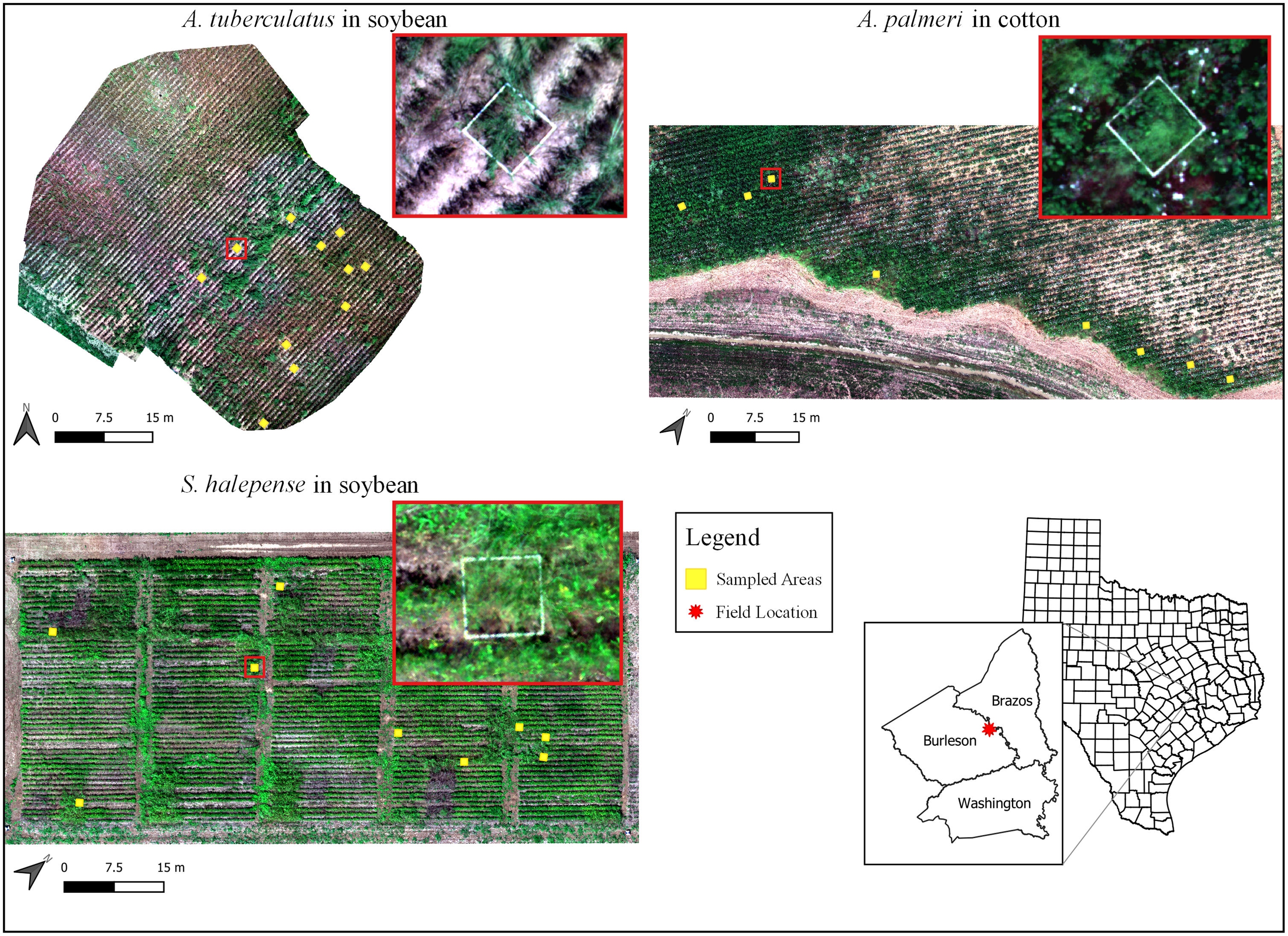
Figure 1. Overview of the three field experiments conducted at the Texas A&M AgriLife research farm, Burleson County, TX. Yellow squares represent locations of the experimental unit setup for each experiment. Insets show the zoomed section of a representative experimental unit (1-m2 quadrat; red boxes).
Table 1. Description of the three field experiments conducted in this study.
a Each experimental unit represents a 1 m by 1 m quadrat.
Image Acquisition
In each experiment, aerial images were collected using the MicaSense RedEdge-M multispectral sensor (MicaSense, Seattle, WA) mounted on a DJI Matrice 600 Pro (DJI, Shenzhen, China) UAV, as well as a high-resolution RGB camera mounted on a DJI Phantom 4 Pro UAV, approximately 2 to 3 wk before crop harvest when weeds reached seed maturity. For each flight, radiometric calibration was performed using calibration panels. Two separate flights were made on the same day with the two UAV platforms. The aerial images were acquired by flying in a grid pattern, with side and end overlaps of 80%. Flights were performed within 2 h of solar noon and on days with little to no cloud cover. The wind speeds were within the normal range (6 to 10 km h−1) during image acquisition for all the experiments.
Ground Truth Data
Ground truth data were collected on the same day of image acquisition (after the flights), using multiple 1-m2 quadrats (Table 1) placed in the experimental area before the flights in a stratified random sampling manner to account for different density gradients of weed species across the field. Each field had good distribution of the target weed species, and the samples harvested contained only the target weed. The quadrats were made of 1.27-cm-diameter white PVC pipes for easy detection in the aerial imagery (see Figure 1, insets). Quadrats were placed such that at least one crop row was contained within. Crop rows were spaced 76 cm apart, and the planting densities were 86,000 seeds ha−1 for cotton and 300,000 seeds ha−1 for soybean. In each quadrat, the total number of the target weed species was counted, ground coverage (%) by the weed within the quadrat was estimated, mature inflorescences were collected, and shoot biomass was harvested at the ground level. Before mature inflorescences were collected, percent seed shattering (for S. halepense only) was recorded based on visual rating (0% to 100%), with 0% being no shattering loss and 100% being complete seed loss. Seed shattering for S. halepense was 20% on average for the 11 collected samples.
Weed samples harvested within each quadrat (i.e., inflorescence, shoot) were placed in separate brown bags and dried in an oven at 60 C for 72 h and then weighed; the sum of the shoot dry weight plus dry inflorescence weight provided the total biomass weight. All mature inflorescences were threshed and cleaned using the South Dakota seed blower (Seedburo Equipment Company, Des Plaines, IL), and remaining debris was separated using a stack of sieves until seeds were not further separable from plant residue. Seed numbers within each sample were estimated based on average 1,000-seed weight, determined using three aliquots for each sample. The total seed number was adjusted based on any shattering that had already occurred.
Image Preprocessing
Both RGB and multispectral images acquired for each experiment were processed and stitched using the Pix4D software (Pix4Dmapper, Lausanne, Switzerland) to produce orthomosaic imagery. For multispectral images, radiometric correction was performed using the calibrated reflection panels and specifying the Camera and Sun Irradiance option in Pix4D. The DSM and digital terrain model (DTM) generation were enabled during multispectral image mosaicking and were used as precursors of the CHM. The structure from motion algorithm that makes use of a Scale Invariant Feature Transform feature detector to generate dense point clouds from a series of overlapping 2D images (Lingua et al. Reference Lingua, Marenchino and Nex2009) was used to produce the DSM and DTM layers in this study. Thus, for each experiment, four UAV-based remote sensing products were generated: (1) an RGB orthomosaic, (2) a calibrated multispectral orthomosaic, (3) a multispectral sensor-derived DSM, and (4) a multispectral DTM. These were used for further processing and calculation of VIs and the CHM.
Calculation of Remote Sensing Variables
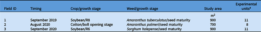
Following the generation of orthomosaics (Figure 2A), several remote sensing variable layers, including NDVI (Figure 2B) and ExG, were generated using Equations 1 and 2, respectively. Two different ExG layers were generated using the RGB and multispectral sensor bands, hereafter referred as “RGB-ExG” (Figure 2C) and “Multi-ExG” (Figure 2D), respectively. Additionally, CHMs were calculated using DSMs and DTMs, following Equation 3. The quadrats were located in the orthomosaic imagery, and the canopy of the target weed species growing within each quadrat was manually outlined by creating polygon features (Figure 2F) in ArcGIS Pro (v. 2.6; Esri 2019, www.esri.com). After canopy delineation, the remote sensing variable layers were clipped to the canopy boundary, and the clipped layers were then subjected to trial/error-based thresholding to remove non-target areas. The non-target areas within the clipped layers included soil background and crop debris underneath the plant canopy. For NDVI, a threshold was set at 0.2 for both NIR and NDVI, and any pixel value lower than the threshold value was eliminated. For the CHM, the threshold was set at 20 cm. A threshold of 0.1 was used for RGB-ExG, whereas it was set at 0 for Multi-ExG; ExG thresholds were set by visual inspection, which slightly differed due to differences in spatial resolution and radiometric response of the two sensor types. Further, any contour <400 cm2 was also eliminated. During thresholding, the unwanted pixels within the canopy were assigned null values, while the remaining pixels retained their original values. Cumulative values of NDVI, RGB-ExG, Multi-ExG, and canopy volume estimates were then calculated using Equations 4, 5, and 6, respectively.
 $${\rm{NDVI}} = {\rm{ }}{{\left( {{\rm{NIR}} - {\rm{Red}}} \right)} \over {\left( {{\rm{NIR}} + {\rm{Red}}} \right)}}$$
 $${\rm{ExG}} = {\rm{ }}{{\left( {2 \times {\rm{Green}} - {\rm{Red}} - {\rm{Blue}}} \right)} \over {\left( {{\rm{Blue}} + {\rm{Green}} + {\rm{Blue}}} \right)}}$$
 $${\rm{CHM}} = {\rm{DSM}} - {\rm{DTM}}$$
 $${\rm{Cumulative\;NDVI}}\; = \mathop \sum \nolimits_{{\rm{i}} \in {\rm{Canopy\;area}}} \;\;\;{\rm{NDV}}{{\rm{I}}_i}$$
 $${\rm{Cumulative\;ExG\;}} = \mathop \sum \nolimits_{{\rm{i}} \in {\rm{Canopy\;area}}} {\rm{\;\;\;Ex}}{{\rm{G}}_i}$$
 $${\rm{Canopy\;volume\;}} = \mathop \sum \limits_{{\rm{i}} \in {\rm{Canopy\;area}}} {\rm{CH}}{{\rm{M}}_i}{\rm{\;}} \times {\rm{\;Cell}}_{{\rm{size}}}^2$$
where i indicates the ith pixel in the canopy area.
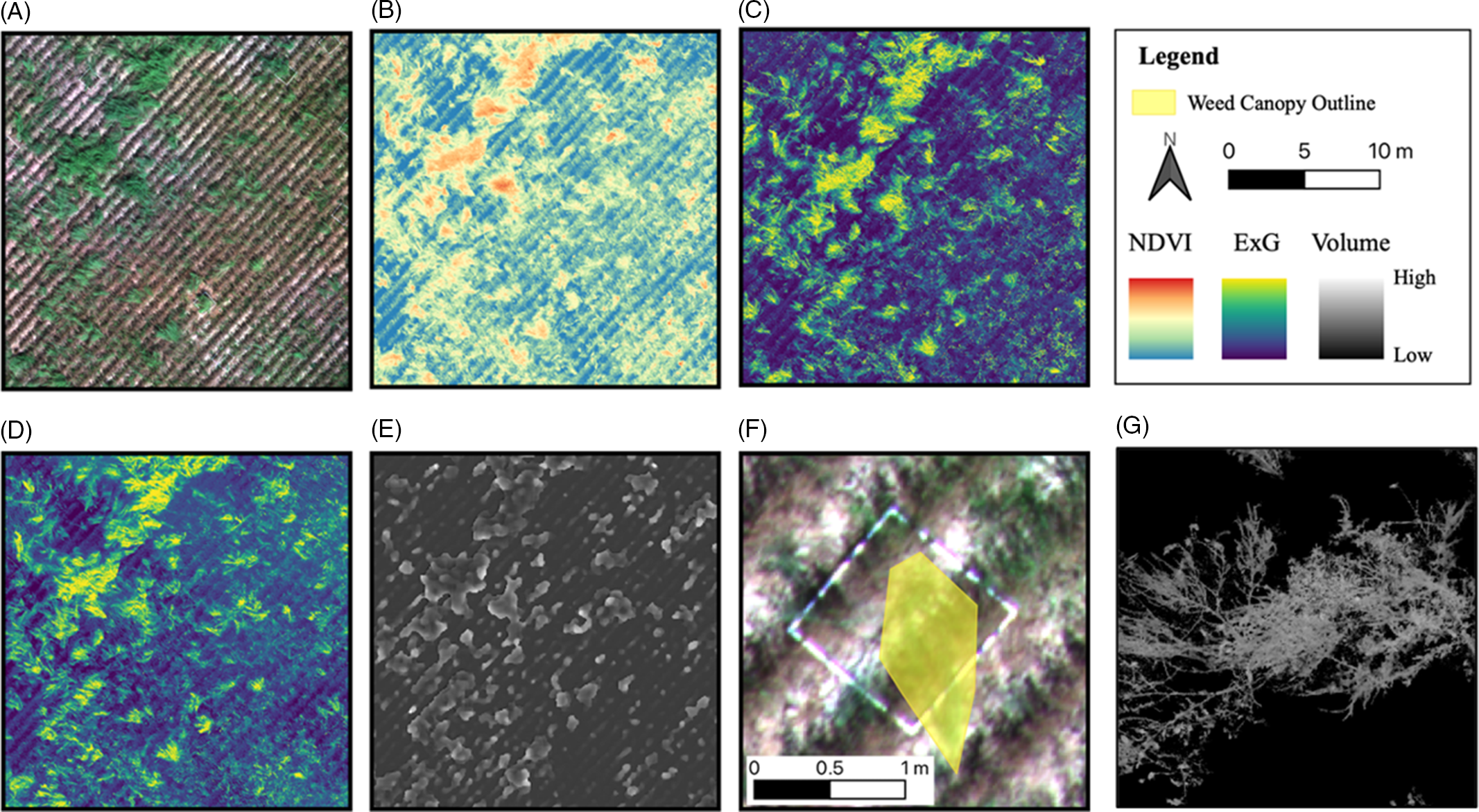
Figure 2. Steps followed in this study in estimating weed seed production using remote sensing: (A) generation of an orthomosaic; (B–D) creating vegetation indices (VIs): (B) normalized difference vegetation index (NDVI), (C) RGB-ExG, and (D) Multi-ExG; (E) estimating canopy volume using the canopy height model (CHM); (F) outlining the weed canopy area; and (G) thresholding VIs and volume estimates. ExG, excess green index.
Correlation Analysis
Because the goal of this study was to investigate the potential of remote sensing variables in estimating seed production in weed escapes, the magnitude and direction of the relationships between the ground truth data (weed seed count) and values estimated using remote sensing variables were investigated. The Pearson correlation analysis was conducted using the R programming language (R Core Team, Vienna, Austria). The correlation coefficient ranges between −1 and 1, and coefficient values away from 0 and closer to 1 indicate strong positive (+) or negative (−) relationships between the variables.
Results and Discussion
VIs versus Canopy Volume
Canopy volume estimates showed stronger association with seed production estimates than VIs for two out of the three weed species studied. Seed production was more closely related to canopy volume estimates for A. palmeri and S. halepense (r = 0.87 and r = 0.90, respectively) (Figure 3B and C), whereas for A. tuberculatus, NDVI had the strongest relationship with seed production (r = 0.81) (Figure 3A; Table 2). Sorghum halepense typically grows tall with an open canopy and high biomass production; ground truth biomass was weakly correlated in this species with canopy volume estimates (r = 0.78) and seed count (r = 0.77). The relatively weak correlation observed here may be attributed to high overlap among tall plants (Figure 1, inset), which corroborates the findings of Watanabe et al. (Reference Watanabe, Guo, Arai, Takanashi, Kajiya-Kanegae, Kobayashi, Yano, Tokunaga, Fujiwara, Tsutsumi and Iwata2017), who also had difficulty measuring the height of grain sorghum [Sorghum bicolor (L.) Moench] (tall crop), but not barley (short crop). It appears that canopy volume, which accounts for tiller spread, is a more reliable predictor (r = 0.9) of seed production in S. halepense than biomass (r = 0.77), though this relationship needs to be verified across multiple populations.
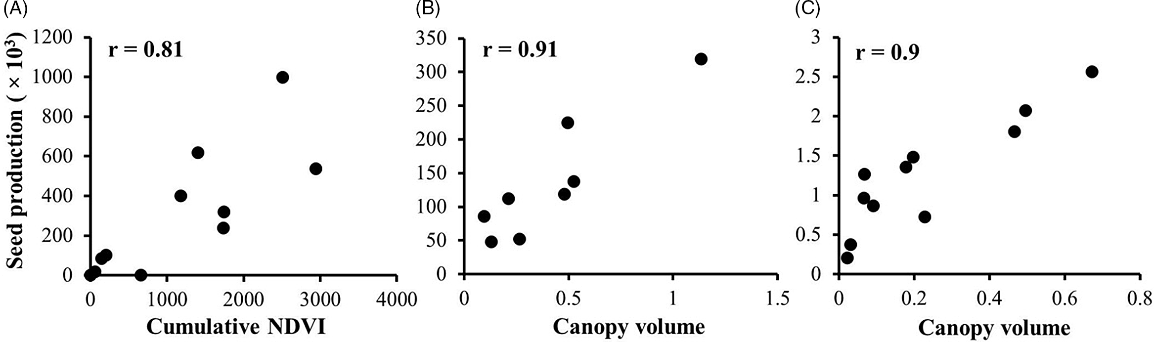
Figure 3. Steps followed in this study in estimating weed seed production using remote sensing: (A) generation of an orthomosaic; (B-D) creating vegetation indices: (B) NDVI, (C) RGB-ExG, and (D) Multi-ExG; (E) estimating canopy volume using CHM; (F) outlining the weed canopy area; and (G) thresholding VIs and volume estimates.
Table 2. Correlation coefficient (r) between ground truth data (weed biomass and seed count) and remote sensing variables.a
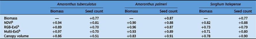
a Abbreviations: ExG, excess green index; NDVI, normalized difference vegetation index.
b Three vegetation indices were included; NDVI and Multi-ExG were generated using a multispectral sensor, while RGB-ExG was created using an RGB sensor.
Among the two Amaranthus species, A. palmeri showed much stronger correlation between ground truth biomass and seed count (r = 0.87), compared with A. tuberculatus (r = 0.77) (Table 2). The reason for the relatively weaker correlation between canopy volume/biomass and seed production in A. tuberculatus compared with A. palmeri is unclear. It is possible that taller seed heads, larger leaf area, and longer petioles of A. palmeri compared with A. tuberculatus (Horak and Loughin Reference Horak and Loughin2000; Sellers et al. Reference Sellers, Smeda, Johnson, Kendig and Ellersieck2003) played an important role here.
With respect to biomass prediction, VIs had stronger correlations than canopy volume estimates for all three weed species. The best VI, however, differed among the species: Multi-ExG, RGB-ExG, and NDVI were the best predictors of biomass for A. tuberculatus (r = 0.97), A. palmeri (r = 0.96), and S. halepense (r = 0.82), respectively (Table 2). Overall, VIs were more accurate for estimating biomass for all three species, whereas canopy volume was more suitable for estimating seed production in A. palmeri and S. halepense. Nevertheless, VIs were better at predicting seed production than plant biomass.
Comparison among the VIs
Among the different VIs evaluated, NDVI had the strongest relationship with seed production in A. tuberculatus and biomass yield as well as seed production in S. halepense, whereas RGB-ExG was found to be the most suitable for A. palmeri biomass, and the Multi-ExG was the most effective for A. tuberculatus biomass as well as A. palmeri seed count (Table 2). The ExG obtained with the two sensor types (RGB vs. multispectral) differed in values, partially because the image-processing pipeline within the RGB sensor involves color transformation and nonlinear encoding (Ramanath et al. Reference Ramanath, Snyder, Yoo and Drew2005).
Feasibility Assessment
The three case studies presented here show that remote sensing–based variables can be used as an efficient alternative to manual estimations of weed seed rain; remote sensing approaches are time- and cost-effective, especially when applied in large production fields. Significant time and labor can be reduced with remote sensing approaches, considering the time it takes for traditional methods in harvesting representative field areas, drying the samples, and counting seeds. Visual estimations of spatial distributions of weeds across vast production fields is an additional challenge. For the remote sensing approach, image collection, preprocessing, and analysis could be accomplished within 72 to 96 h for an average hectare area. However, the actual time and cost incurred can be influenced by multiple variables.
Among the remote sensing approaches investigated here, multispectral variables were generally more robust compared with RGB imagery, but RGB sensors are cost-effective and in many cases may be sufficient. Though the cost of multispectral sensors has dropped significantly over the years, it is still about 10 times the average cost of an RGB sensor. Moreover, consumer-grade UAV platforms that integrate RGB sensors have become widely accessible and are much cheaper compared with platforms used with multispectral sensors. Unlike multispectral sensors, the consumer-grade RGB-based drones offer ease of use to practitioners. Further, image-processing workflows have become more standardized with over-the-counter software packages tailored to widely available RGB sensors. However, the time required for image analysis does not significantly differ between the two sensors. Thus, low-cost RGB-based imagery has the potential to aid researchers, extension agents, and farmers in determining seed rain potential in uncontrolled weed escapes and tailoring management that meets seedbank reduction goals.
This study provides novel insights into how remote sensing–based variables, like VIs and canopy volume, can replace conventional approaches for estimating weed biomass and seed count. The goal of this study was to determine whether remote sensing can be an efficient alternative to manual estimations of seed production in weed escapes, not to identify the best predictor for each of the weed species investigated. The three weed species and associated crops served as valuable case studies to understand the potentials and limitations of using simple remote sensing approaches for weed seed rain estimation. Our results clearly show that the choice of the best remote sensing approach may vary across production scenarios, and here we provide select examples of how and in what cases certain variables performed the best. Further research is required to shed more light on the best approach to adopt.
Major limitations exist for using remote sensing–based variables to estimate weed biomass and seed count. In this study, the female plant canopies were manually identified in situ and delineated in aerial images using GIS software. This process is burdensome and difficult to scale up across large areas. Moreover, both male and female plants typically coexist in the field and exhibit highly similar morphological characteristics (Keeley et al. Reference Keeley, Carter and Thullen1987). Females have rough inflorescences with spines located in bracts, whereas males have soft inflorescences and spineless bracts (Spaunhorst and Johnson Reference Spaunhorst and Johnson2017). These subtle differences are difficult to detect using traditional remote sensing and likely require an advanced machine learning approach.
A notable machine learning approach is to utilize convolutional neural networks to detect and segment out just the female seed head in RGB images. These neural network models have been successfully used for various detection and localization tasks, including identifying rice (Oryza sativa L.) panicles (Xiong et al. Reference Xiong, Duan, Liu, Tu, Yang, Wu, Chen, Xiong, Yang and Liu2017) and counting grain sorghum panicles (Malambo et al. Reference Malambo, Popescu, Ku, Rooney, Zhou and Moore2019). These techniques can be adequately applied to estimate and measure the seed heads for several weed species, including the target species in this study. The detection results can be coupled with seed count regression models to estimate seed count at the desired scales. While these techniques have great promise, it should be noted that they are technically complex and require high computational power.
Overall, this study proves the concept that UAV-based remote sensing holds great promise for seed rain estimation from uncontrolled weed escapes. This information can be used to generate field maps of seed rain potential, which can be utilized for precision management with drone-based treatments or harvest weed seed control tactics. For drone-based applications, estimations of seed rain potential before seed production can be more useful. Additional experiments are required to better understand the relative importance of different remote sensing variables for estimating seed rain potential for the weed species of interest in a given geography.
Acknowledgments
This research was financially supported in part by USDA-NRCS-Conservation Innovation Grant (CIG) program (Award # NR213A750013G017) and Cotton Incorporated.
The authors declare that no conflicts of interest exist.


 Open access