


Introduction
The mass balance of an ice sheet (the amount by which its mass increases or decreases) has important consequences for sea level, but until recently it was not possible even to determine whether the big ice sheets in Greenland and Antarctica were growing or shrinking. Over the past decade, improved remote-sensing techniques combined with accurate GPS (global positioning systems) have made it possible to estimate ice-sheet mass balance in three independent ways: the mass-budget approach, comparing total snow accumulation with total losses by melting and ice discharge; the altimetry approach, using time series of precise altimetry surveys to measure rates of surface-elevation change and to infer volume changes; and the gravity-change approach, using satellite measurements of temporal change in gravity to estimate changes in ice mass. These have resulted in numerous mass-balance estimates, particularly for Greenland (Fig. 1).
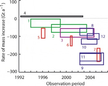
Fig. 1. Rates at which the mass of the Greenland ice sheet has been estimated to be changing based on European Remote-sensing Satellite (ERS) SRALT data (black), airborne laser-altimeter surveys (green), airborne/satellite laser-altimeter surveys (purple), mass-budget calculations (red) and temporal changes in gravity (blue). Rectangles depict the time periods of observations (horizontal) and the upper and lower estimates of mass balance (vertical). Sources (corresponding to numbers on rectangles): 1 and 2: Reference KrabillKrabill and others (2000, Reference Krabill2004); 3: Reference Thomas, Frederick, Krabill, Manizade and MartinThomas and others (2006); 4: Reference ZwallyZwally and others (2005); 5–7: Reference Rignot and KanagaratnamRignot and Kanagaratnam (2006); 8 and 9: Reference Velicogna and WahrVelicogna and Wahr (2005, Reference Velicogna and Wahr2006); 10: Reference RamillienRamillien and others (2006); 11: Reference Chen, Wilson and TapleyChen and others (2006); 12: Reference LuthckeLuthke and others (2006).
In marked contrast to other estimates, results from satellite radar-altimetry (SRALT) data (Reference ZwallyZwally and others, 2005) indicate ice-sheet growth, with a remarkably small estimated error, during a period when other approaches show substantial losses. SRALT data provide the longest available altimetry time series over ice sheets, and this is likely to be sustained for many years to come. Consequently, it is important to identify the reasons for this discrepancy, to be able to assess the viability of SRALT surveys for monitoring ice-sheet mass balance.
Since 1991, ice-sheet topography has also been measured by airborne laser altimeters, with extensive surveys over Greenland. These provided the first evidence for substantial mass loss, particularly on some of the faster-moving outlet glaciers (Reference KrabillKrabill and others, 2000). Since 2003, a laser altimeter aboard NASA’s Ice, Cloud and land Elevation Satellite (ICESat) has provided similar data, and here we compare SRALT estimates of elevation-change rates (dS/dt) with those derived from the laser altimeters, and we offer possible explanations for differences between them.
Altimetry Techniques
Satellite radar altimeter (SRALT)
Accurate SRALT data were first acquired over ice sheets (up to latitude ±72°) in 1978 by NASA’s Seasat and the US Navy’s Geosat (1985–89). The European Space Agency’s ERS-1 (1992–95), ERS-2 (1995–2003) and Envisat (2003–present) satellites have provided continuous coverage of the ice sheets up to ±81.5° latitude over the last 15 years. These radar altimeters, with antenna beam widths of ∼20 km, were designed and demonstrated to make accurate measurements over the almost flat, horizontal ocean. Data interpretation is far more complex over sloping and undulating ice-sheet surfaces with spatially and temporally varying dielectric properties, which affect backscatter intensity and radar penetration into the snow (Reference Legrésy and RémyLegrésy and Rémy, 1998; Reference Arthern, Wingham and RidoutArthern and others, 2001). Range measurements are made to the closest region within the large footprint, introducing an elevation error proportional to surface slope. In principle, this can be corrected, but undulations and valleys can introduce additional errors which cannot be corrected. As far as we are aware, techniques for correcting the effects of temporally varying radar backscatter and penetration into the snow have not been validated.
SRALT-derived topography over smoother, low-slope parts of the Greenland ice sheet has been compared with that from other measurements (Reference Ekholm, Bamber and KrabillEkholm and others, 2002) to reveal overall agreement to within a few metres after correction for surface slopes. This uncertainty is a measure of residual slope effects and, perhaps, radar penetration into the snow. Estimates of dS/dt are made at locations where a satellite orbit crosses one from an earlier period, assuming that topography-induced errors are the same for each measurement. For a continuous series of elevation measurements, an elevation time series at crossing points is used to infer an average dS/dt at each crossing point location over the entire survey period.
Airborne Topographic Mapper (ATM)
The ATM is a conically scanning laser altimeter that accurately surveys the surface topography of a swath of terrain directly beneath the path of the aircraft. It comprises the scanning laser with associated optics and data system, a differential GPS system for accurate positioning of the aircraft, and accelerometers and gyros to measure aircraft roll, pitch and heading. Using these three systems, each individual laser pulse, or ‘shot’, is assigned three-dimensional geographic coordinates. With thousands of these shots fired each second, the result is a topographic survey of a swath of width ranging between 400 and 1200 m, depending on aircraft height (typically 500–1500 m) and off-nadir scan angle.
Shot density within the surveyed swath yields one measurement of a ∼1–3 m footprint for every few square metres. In addition to this high-volume data product, a far more compact dataset is produced by fitting 70 m planar surfaces, adjacent across the swath and overlapping along track. These ‘platelets’ are described by centre coordinates, vector slope and rms fit of the ATM data to a plane (effectively the ice surface roughness). The polar ice sheets are sufficiently smooth and flat over >90% of their area for this compact dataset to contain all desired information. For change detection, laser swaths are re-surveyed after a few years, and differences between the two surveys yield estimates of dS/dt during the interim.
Extensive ATM surveys were made of the Greenland ice sheet in 1993/94 and again, along the same flight-lines, in 1998/99 (Reference KrabillKrabill and others, 2000). These showed slow overall thickening above 2000 m elevation, but quite rapid thinning nearer the coast. The 1993 and 1998 surveys were made over the southern part of the ice sheet in June/July at the height of the melt season, and those in 1994 and 1999 were made during May, near the start of the ablation season.
Geoscience Laser Altimeter System (GLAS)
NASA’s ICESat was launched in January 2003, carrying GLAS, a laser altimeter with three lasers to be operated sequentially in order to achieve a mission lifetime of 3–5 years. GLAS is a nadir-looking sensor with a pulse repetition rate of 40 Hz, footprint diameter of ∼70 m and separation of 170 m (Reference ZwallyZwally and others, 2002). Its prime objective is to measure the rate of change of surface elevation on the Greenland and Antarctic ice sheets. Data acquisition began in February 2003, but laser-1 prematurely failed after operating for 37 days in an 8 day repeat orbit. In order to conserve the lifetime of the remaining two lasers, it was decided to adopt a strategy whereby the active GLAS laser would complete a 33 day subcycle of a 91 day repeat orbit and then be switched off intermittently to conserve its life.
Following this plan, laser-2 was activated in September 2003, and, after completing one 8 day cycle, ICESat was shifted to the 91 day repeat orbit for 54 days, with the 33 day subcycle completed after mid-October selected for future repeat surveys. This 33 day sequence has been repeated using laser-2 then laser-3 during February/March, May/June and October/November each year since, along the same orbit tracks, with the May/June survey omitted in 2007.
Methods
Our aim here is to compare estimates of dS/dt over Greenland from ERS data with those from laser altimeters. For the laser estimates, we compared elevations derived from GLAS and ATM over many locations on the ice sheet, and averaged the resulting differences within 50 km grids. For the radar estimates, time series of dS/dt values for 1995–2003 were computed from ERS-2 data at crossover locations that occur at clearly defined spatial intervals associated with the 35 day exact repeat satellite orbit. Separation between crossover locations decreases with increasing latitude, and varies from 35 km at 66° N to 10 km at 80° N. Time series were formed consistent with procedures described by Reference Li and DavisLi and Davis (2006). After time-series formation, a least-squares fit was used to estimate the average rate of elevation change over the specified time periods (Fig. 2).
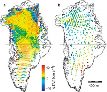
Fig. 2. Rates of elevation change (dS/dt) (a) from ERS-2 and (b) from GLAS/ATM, for 1998/99 to 2003.2. The black line across the middle of the ice sheet marks the boundary separating data from June/July 1998 to February 2003 in the south and those from May 1999 to February 2003 in the north.
Most complete ATM surveys were made in 1993/94 and 1998/99, with ERS-1 operating during the first of these periods, and ERS-2 during the second. In order to avoid problems associated with biases between the two ERS sensors, we chose to use results from only ERS-2, which provided useful data between June 1995 and May 2003. Consequently, we compared dS/dt from ERS-2 with equivalent values inferred from elevation changes during the interim between surveys in the 1990s by ATM and those by ICESat, which began operating in February 2003.
At higher elevations, where there are many data from all three sensors, and values of dS/dt are reasonably well correlated over quite large distances, we binned and averaged values of dS/dt from ERS and from ATM/ICESat into 50 km grid squares, and compared the resulting estimates of dS/dt for approximately the same time periods. At lower elevations, this approach is not viable because of sparse data coverage and very high spatial variability of dS/dt. Consequently, we focused attention on Jakobshavn Isbræ, where a series of ATM surveys in a grid pattern provide spatially detailed estimates of dS/dt between 1997 and 2002 for comparison with estimates from ERS-2 over the same period within the region covered by the ATM surveys.
In order to compare elevations derived from ATM with those from ICESat, we had to take account of differences between the footprint sizes of the two lasers. Overlapping (by 50%) flat ‘platelets’ were fitted to the ∼1200 aircraft measurements on each side of the aircraft within a 70 m along-track distance, generally with rms fit of 10 cm or less, representing the effects of shot-to-shot noise, ice-surface roughness and the small surface curvature at higher elevations. These were compared with ICESat footprint elevations by extrapolating elevations from any platelet within 200 m of the GLAS-footprint centre using the platelet slope. This generally yielded four comparisons for each GLAS footprint, and these were averaged to give the GLAS/ATM comparison for that footprint (Fig. 2).
Surface elevations on the Greenland ice sheet have a strong seasonal cycle, so dS/dt comparisons are best made over identical periods. This was done for 1998–2003 for the southern part of the ice sheet and for 1999–2003 in the north. We also compared dS/dt from ERS-2 and laser-survey periods that overlapped (three in the south and four in the north), with the laser period starting or ending as nearly as possible in the same season as the ERS-2 period in order to minimize seasonal effects. Most of the ice sheet covered by these comparisons has comparatively small surface slopes, and poorly represents the outlet glaciers, where most of the recently observed changes have occurred. Consequently, we also compared dS/dt estimates from parts of Jakobshavn Isbræ and its catchment basin, with quite rough surface topography and high thinning rates.
Results
Higher elevations
Our ATM surveys covering the ice sheet were made in June/July 1993 and 1998 over the southern part of the ice sheet, and during May 1994 and 1999 in the north. We compared the resulting 1994–99 dS/dt values with those from ERS-2 for 1995–99, and for eight other time intervals we compared dS/dt from ATM/GLAS comparisons with those from ERS-2, omitting all data from elevations less than 1500 m.
Figure 2 shows ERS- and laser-derived estimates of dS/dt for the surveys over identical time periods. Both sets of results have very similar patterns, but the ERS estimates show stronger thickening, except in the southeast, where laser estimates show more thickening. This may be related to the exceptionally high snowfall in this region shortly before the 2003 measurements (Reference KrabillKrabill and others, 2004; Reference Hanna, McConnell, Das, Cappelen and StevensHanna and others, 2006). Radar penetration into the resulting low-density thick layer of dry winter accumulation may have been deeper than normal, resulting in anomalously low SRALT-derived elevations.
Spatial variability near the coast is very large, where results are heavily affected by sample location. Consequently, the dS/dt estimates from all nine comparisons were binned and averaged into 50 km grids for all ice-sheet elevations above 1500 m. The gridded laser averages were then subtracted from the gridded ERS averages. Resulting differences (ΔdS/dt) for the surveys in Figure 2 are shown in Figure 3. Most values are positive, indicating that ERS-derived dS/dt values are more positive than laser-derived ones.

Fig. 3. Difference in estimates of dS/dt shown in Figure 2; ΔdS/dt = ERS values minus laser values.
Similar results were found from all four comparison periods in the south and from those in the north (Table 1), but spatial variability of ΔdS/dt, combined with differences between sampling locations and density, for ERS and for laser, introduce errors on individual grid values. These are uncorrelated over large regions, so we averaged values over large areas defined by elevation limits. Results are summarized in Figure 4 as differences, from each of the nine comparisons, between the two sets of estimated rates of elevation change averaged over all elevations above 1500, 2000, 2500 and 3000 m. In almost every case, ERS-derived average dS/dt is higher than from the laser altimeters, with differences ranging from ∼1 to >10 cm a−1.
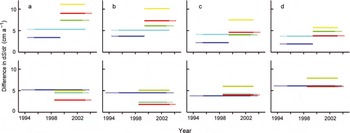
Fig. 4. Values of ΔdS/dt measured over different time periods, with values averaged over all elevations: (a) >1500 m; (b) >2000 m; (c) >2500 m; and (d) >3000 m. The ERS time period is depicted by the solid line; that for the laser comparisons is the union of solid and dotted line. The upper series of plots is from the north of the ice sheet; the lower series is from the south.
Table 1. Differences (ΔdS/dt) between ERS SRALT and GLAS/ATM laser estimates of rates of ice-surface elevation change over a range of time periods; those marked with an asterisk compare ERS and laser estimates over identical periods. Dates are given in years and decimals. Error estimates are explained in the Appendix. Coverage was too sparse over the southern part of the ice sheet at elevations below 2000 m to provide reliable results
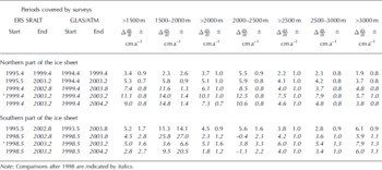
Figure 4 shows an increase of ΔdS/dt with time in the north, but no clear trend in the south. However, the early values of ΔdS/dt are based on comparison of ERS results beginning in 1995 with laser results starting in 1994 in the north and 1993 in the south, and may have large errors associated with interannual variability in snowfall. Comparisons after 1998 (italics in Table 1) cover time periods that differ by no more than 1 year, with one having identical ERS and laser time periods. Results here, for the various elevation bands, show agreement consistent with estimated errors and the 1 year mismatch between some of the radar/laser comparisons. It is notable that values of ΔdS/dt are, in most cases, highest for the year with identical radar and laser time periods (marked with an asterisk in Table 1). We averaged results for each elevation band from all three later comparisons in the south, and for those in the north, to provide estimates of average ΔdS/dt, shown in Figures 5 and 6, for 1998/99–2003, along with estimated errors (see Appendix).

Fig. 5. Values of ΔdS/dt averaged overall elevations >1500, >2000, >2500 and >3000 m for the north (blue) and the south (red) of the ice sheet from all comparisons after 1998. The shading indicates estimated errors (see Appendix).
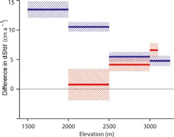
Fig. 6. Values of ΔdS/dt (blue in the north; red in the south) averaged from comparisons after 1998 within 500 m elevation bands, plotted against surface elevation. The shading indicates estimated errors (see Appendix).
Figures 5 and 6 show very large values of ΔdS/dt averaged over the northern ice sheet above 1500 m, with a progressive decrease in average ΔdS/dt at higher elevations. In the south, average ΔdS/dt is effectively the same as in the north for elevations above 2500 m, and far less at lower elevations, but with quite large uncertainty.
Part of the increase in northern values of ΔdS/dt with decreasing elevation is probably the effect of topography. Many of the ATM surveys were along outlet glaciers that were found to be thinning more rapidly than nearby ice, so the laser estimates of dS/dt are very probably biased towards thinning. However, the catchment basins of these glaciers are undulating, with topographic highs and lows within an ERS radar footprint. In such areas, SRALT-derived elevation changes are questionable because radar-altimeter processing uses information primarily from the return-pulse leading edge, which represents radar reflections from the highest-elevation parts of the footprint. This problem is examined in more detail in the Discussion.
Near-coastal regions
Estimates of dS/dt from ATM surveys in 1997 and 2002, along a grid network of flight-lines, were interpolated to give 1 km gridded values for 12 600 km2 of Jakobshavn Isbræ and its catchment basin shown in Figure 7. Locations of ERS-2 orbit crossing points where associated values of dS/dt over the same period were calculated are also shown. We compared each of these with the average ATM-derived value for a 3 km by 3 km area centred on the crossover location (Table 2).
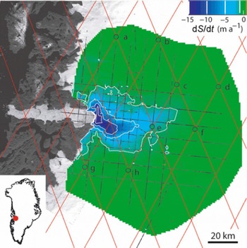
Fig. 7. Jakobshavn Isbræ and part of its catchment basin, showing the grid of ATM surveys made in 1997 and 2002 (thin black lines), from which values of dS/dt (depicted by the colour scale) were inferred, with white contours at dS/dt = −1, −5, −10 and −15 m a−1. Coloursin the small circles show dS/dt estimates from time series of SRALT measurements at crossing points (a–h) of ERS-2 orbits (thin red lines). SRALT data at the other crossing points were too badly affected by rough surface topography to yield estimates of dS/dt.
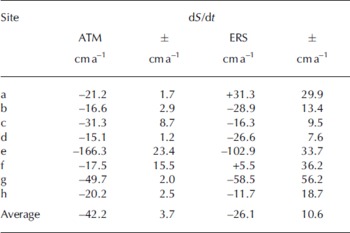
Table 2. Estimates of dS/dt between 1997 and 2002 derived from ATM surveys and from SRALT data at ERS orbit-crossing locations over Jakobshavn Isbræ shown in Figure 7. Error estimates are a measure of the spatial variability of dS/dt along adjacent grid survey lines for ATM, and of the goodness of fit of a straight line to ERS time series, all assumed to be independent at each site in calculating errors on average values
Although most ATM values in Table 3 show more thinning than the ERS estimates, ERS-estimated thinning is actually higher at three sites where thinning is most rapid, and exclusion of site a would bring the averages into quite good agreement. Indeed, most of the differences between ATM and ERS estimates are of a similar magnitude to the large ERS uncertainty, which is high because of spatial and temporal variability in dS/dt on the rapidly moving glacier. Consequently, where values of dS/dt could be estimated from ERS-2 data, they show agreement within large uncertainty limits with those from ATM. However, at about half of the ERS orbit crossing points in Figure 7, the ERS waveforms over the very rough terrain are too ditorted to calculate dS/dt, and there are no values in the most rapidly thinning region. The overall result is a substantial ERS underestimate of total thinning within the glacier basin, and this almost certainly also applies to other fast-moving glaciers.
Discussion
Reasons for observed bias between radar and laser measurements
Differences between dS/dt estimates from the two techniques, summarized in Table 1 and Figures 5 and 6, are larger than can be explained by the estimated errors. These do not include errors caused by most ERS/laser comparisons not covering identical time periods, but the generally good agreement between the different comparisons suggests that such errors are small and not systematic. The ATM has a well-established heritage, providing accurate measurements of elevation and its change with time (Reference KrabillKrabill and others, 2002), and GLAS-derived elevations have been thoroughly validated against several other independent measurements (Reference Luthcke, Rowlands, Williams and SirotaLuthke and others, 2005; Reference Martin, Thomas, Krabill and ManizadeMartin and others, 2005; Reference Schutz, Zwally, Shuman, Hancock and DiMarzioSchutz and others, 2005). For large-area averages at higher elevations, errors in laser-derived dS/dt are very small (see Appendix). SRALT estimates of errors in large-area averages of dS/dt are also small (Reference ZwallyZwally and others, 2005; Reference Wingham, Shepherd, Muir and MarshallWingham and others, 2006). But SRALT elevations are known to have large slope-induced errors, and corrections must be made for temporally varying radar backscatter. In using SRALT data to estimate dS/dt, it is assumed that slope-induced errors and radar-penetration effects do not change with time at each crossing point, and that adequate corrections have been made for radar-backscatter variability. These effects, together with those of radar penetration into the snow, may introduce a bias into SRALTderived values of dS/dt that is not taken into account in the error estimates.
As far as we are aware, this study represents the first attempt to validate SRALT-derived dS/dt against independent estimates over time periods similar to those covered by the SRALT data. Our results reveal significant differences between SRALT and laser estimates, which most probably represent a SRALT bias caused by progressive lifting of the radar-reflecting horizon within the ice-sheet surface. There is summer melting over about half of the Greenland ice sheet, and this has a large impact on the dielectric properties of surface snow and underlying firn. Because of this, summer melting can be mapped from satellite measurements of microwave emissions and radar backscatter from the snow. Moreover, radar backscatter measurements are also strongly affected by ice lenses and ice layers in the underlying firn, formed by refreezing of surface meltwater that percolates downwards. Consequently, it should not be surprising if SRALT-derived estimates of dS/dt are affected by changes in the area and intensity of summer melting. A time series of melt area on the ice sheet derived from satellite passive microwave measurements is shown in Figure 8, and it is clear that this area has grown substantially since 1979, when measurements began. It is quite probable that this resulted in changes to the properties of the ice-sheet surface that caused a progressive upward shift of the effective radar-reflecting horizon, and SRALT overestimation of dS/dt.

Fig. 8. Maps showing minimum and maximum extent of seasonal surface melt extent (red) on the Greenland ice sheet, which has been observed by satellite since 1979 and shows an increasing trend. The melt zone, where summer warmth turns snow and ice around the edges of the ice sheet into slush and ponds of meltwater, has been spreading inland to progressively higher elevations in recent years (Reference Steffen, Nghiem, Huff and NeumannSteffen and others, 2004).
Our results show SRALT-derived dS/dt to be 1–14 cm a−1 higher than those from laser altimetry for elevations above 1500 m, with highest values at lower elevations and in the north. The increasing trend at lower elevations in the north probably results from upslope migration of summer melting to elevations above 1500 m, combined with a higher concentration of surface undulations. The small values of ΔdS/dt at low elevations in the south could result from these regions already undergoing summer melt at the beginning of survey periods, with radar-reflecting horizons already lifted above dry-snow conditions. However, the estimates of ΔdS/dt ∼ 5 cm a−1 at >2500 m elevation, and generally higher values in the north, are surprising because these are regions associated with dry-snow conditions. A possible explanation is that the dielectric properties of dry snow are more highly sensitive to small melting events than snow with a history of melt events. Such brief periods of melting can extend to very high elevations, and are not represented in maps of melt extent inferred from passive-microwave data (personal communication from K. Steffen, 2007). If this interpretation is correct, recent warming has increased the frequency of such events. Alternatively, some change in dry-snow characteristics may have lifted the radar-reflecting horizon. Radar return-pulse waveforms from high-elevation parts of Antarctica are affected by various characteristics of the snowpack, such as snow density, distribution of ice, wind-crust and depth-hoar layers (Reference Legrésy and RémyLegrésy and Rémy, 1998), and by wind-induced surface roughness (Reference Legrésy, Rémy and ShaefferLegrésy and Rémy, 1999). It is quite possible that progressively warmer Greenland summers have caused a secular change in some of these characteristics and a lifting of the effective radar-reflection horizon.
Near the coast, radar penetration into the snow is of far less concern than the local surface topography, which becomes quite rough, particularly in the most active parts of outlet glaciers where thinning rates are highest. Elevation profiles along some of the north–south flight-lines over Jakobshavn Isbræ (Fig. 7) are shown in Figure 9, along with the beam-limited wavefront of the ERS-2 satellite. Information used to infer surface elevations and values of dS/dt from SRALT measurements is primarily from the leading edge of the reflected waveform, which represents reflections from highest-elevation regions within the radar footprint. Reflections from the glacier valley, where ice velocities and thinning rates are highest, lie within the tail of the reflected waveform. Consequently, derived values of dS/dt represent conditions near the summits of undulations within the radar footprint. Moreover, within the 12 600 km2 of Jakobshavn catchment basin mapped by ATM, less than half of the ERS-2 crossing points included SRALT data from which dS/dt estimates could be derived, resulting in serious underestimation of mass loss.
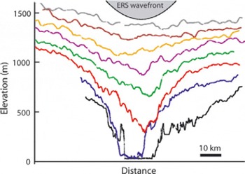
Fig. 9. North–south elevation profiles across Jakobshavn Isbræ from ATM surveys along gridlines shown in Figure 7, with an ERS-2 radar wavefront superimposed. Profiles are taken at ∼7 km separation, with the most seaward (western) at the lowest elevations. The fastest part of the glacier is the region thinning most rapidly in Figure 7, and it flows in a valley that cannot be sampled by the leading edge of the radar pulse.
Impact on mass-balance estimates
The net effect of the mismatch between laser- and radar-derived values of dS/dt can have a very large impact on mass-balance calculations. The area of the Greenland ice sheet above 2000 m elevation is ∼1.5 × 10⁶ km2, implying a volume change of 15 km3 for a 1 cm uniform change in elevation over the entire region. This represents a change in mass of almost 14 Gt cm−1 of solid-ice thickening and ∼6 Gt cm−1 for a recent increase in snowfall. Our results indicate that ERS-derived values of dS/dt between 1998/99 and 2003/04 exceeded those from laser altimeters by ∼8 cm a−1,averaged over the ice sheet in the north above 2000 m elevation (area ∼1 × 10⁶ km2), and by ∼3 cm a−1 in the south (area ∼0.5 × 10⁶ km2). This corresponds to a volume-balance difference of ∼95 km3 a−1,for the entire ice sheet above 2000 m elevation, or a mass-balance difference ranging from 38 Gt a−1, if thickening is caused by recent increases in snowfall (density ∼400 kg m−3), to 86 Gt a−1 for long-term ice thickening (density ∼900 kg m−3).
The longer-term estimates of ΔdS/dt above 2000 m elevation, in Table 1 and Figure 4b (ΔdS/dt ∼ 5 ± 1 cm a−1), better match the time period of published ERS-derived estimates of Greenland mass balance (Reference ZwallyZwally and others, 2005). Using these values, the volume-balance difference for ERS minus laser-derived estimates above 2000 m elevation is ∼75 ± 15 km3 a−1.Reference ZwallyZwally and others (2005) used ATM estimates of near-coastal ice-sheet thinning between 1993/94 and 1998/99, together with ERS-derived estimates of dS/dt at higher elevations, to infer ice-sheet growth of 1 ± 13 Gt a−1 between 1992 and 2002, assuming the density of thickening ice to be 917 kg m−3. Using this same density, our results indicate that laser-derived dS/dt during the same time interval would alter this estimate to a mass loss of almost 60 Gt a−1, with errors assumed to be ±20–30 Gt a−1, similar to those for the other altimeter-based estimates in Figure 1.
It is not surprising that the modified SRALT estimate shows good agreement with the laser-based estimates, because we used the laser results to ‘correct’ the SRALT estimate, but it is also consistent with the mass-balance estimates in Figure 1 that are not based on altimeter measurements, providing support for our conclusions of SRALT overestimation of dS/dt. Indeed the Reference ZwallyZwally and others (2005) Greenland mass-balance estimates would show even more ice-sheet growth if based solely on SRALT data, primarily because SRALT data cannot be used to infer dS/dt over the very rough surfaces typical of outlet glaciers where thinning is most pronounced.
Ramifications for Antarctica
Most outlet glaciers in Antarctica are far wider than in Greenland, so topographic effects should be less severe. Nevertheless, there are also many narrow glaciers flowing between rugged mountains, that are similar to those in Alaska and Greenland. In such regions, SRALT data cannot be used to infer reliable estimates of dS/dt. This is particularly so in the Antarctic Peninsula, where other observations show glacier acceleration and very rapid thinning as ice shelves weaken or break up.
By contrast with Greenland, there is little or no surface melting over most of Antarctica, so errors caused by melt-induced temporal variability of radar penetration should be smaller than in Greenland. But this has yet to be confirmed, and recent observations show summer melting over larger areas in Antarctica than in Greenland, that this area is increasing with time (Reference Nghiem, Steffen, Neumann, Huff, Tregoning and RizosNghiem and others, 2007) and that local warming over the Antarctic Peninsula has exceeded that in most other regions on Earth. Moreover, our results from northern Greenland show substantial SRALT overestimation of thickening rates at high elevations, suggesting that changes in snow characteristics other than melting may also be affecting the radar data. It is instructive to note that a bias of only 1 cm a−1 in dS/dt averaged over the entire 12 × 106 km2 of Antarctica is equivalent to a bias in ice-sheet volume balance of 120 km3 a−1, a value similar in magnitude to estimates of total balance of the ice sheet.
It is highly probable that SRALT estimates of dS/dt from parts of Antarctica will be affected by a melt-induced bias and/or by the changes in dry-snow characteristics reported by Reference Legrésy and RémyLegrésy and Rémy (1998, Reference Legrésy, Rémy and Shaeffer1999). Moreover, the work presented here shows that SRALT bias for Greenland is far larger than 1 cm a−1,and we have yet to estimate its magnitude in Antarctica. Meanwhile, it would be unwise to assume it is zero, and the real uncertainty of existing SRALT-derived estimates of volume balance is probably far larger than published values.
Conclusions
Results presented here indicate SRALT-derived rates of surface-elevation change on the Greenland ice sheet show substantially more thickening at higher elevations than do repeat laser-altimeter measurements, with differences of a similar magnitude to the total imbalance of the ice sheet. We interpret this as an indication of errors in the SRALT measurements, primarily caused by a progressive lifting of the effective radar-reflecting horizon as increasing temperatures affect surface snow characteristics, such as the area and intensity of summer melting. If this is correct, SRALT data cannot be used to estimate ice-sheet mass balance without making corrections for this effect. Such corrections will require a more complete understanding of the influence of snow characteristics on radar backscatter. Even with this understanding, it may be necessary to monitor characteristics, such as snow wetness, layering and surface roughness, that are found to have a strong influence. Meanwhile, comparison of simultaneous GLAS and SRALT dS/dt estimates for both Greenland and Antarctica during different seasons may reveal patterns of ΔdS/dt that could be correlated with weather observations and satellite measurements of snow characteristics. This information might be sufficient to develop an empirical correction.
At lower elevations, rougher surface topography limits our ability to use SRALT data to measure dS/dt reliably, because of the large radar footprint. The European Space Agency’s upcoming CryoSat will overcome this problem, to some extent, by utilizing a smaller effective footprint, but will not resolve problems associated with changing snow characteristics.
Conditions in Antarctica, where there is little surface melting and glaciers are far wider, should favour more reliable SRALT interpretation. However, there are large regions, such as the Antarctic Peninsula, where topography is very similar to coastal Greenland, and there are quite large low-elevation regions elsewhere with extensive summer melting. Moreover, as far as we are aware, there has been no direct comparison of SRALT-derived estimates of dS/dt in Antarctica with those from other techniques. Consequently, at a minimum, we recommend caution in the estimation of errors appropriate to SRALT-derived estimates of Antarctic mass balance.
Finally, it is important to stress that the bias between SRALT and laser estimates of elevation change varies both spatially and temporally, so there is no simple correction.
Acknowledgements
This work was funded by NASA’s Cryospheric Processes Program. We thank the reviewers for helpful comments and suggestions.
Appendix: Measurement and Interpolation Errors
Laser
ATM laser ranges are calibrated on the ground before and after each flight, and by surveying GPS-mapped portions of the airstrip, with in-flight consistency tested by repeat surveys of the same profiles during flight. Comparison with surface optical levelling and GPS profiles on the ice indicates that elevation accuracy is typically ∼10 cm (Reference KrabillKrabill and others, 2002) over flight-lines of 2000 km or more. Perhaps half of this uncertainty results from errors in range measurements and half from errors in aircraft GPS trajectory that are systematic to a flight or to a series of flights, but uncorrelated with others.
As a measure of consistency, comparison of GLAS-derived elevations over almost-horizontal ice-sheet surfaces, at locations where near-contemporary orbits cross, shows rms differences of the order of 10 cm for Antarctica and 15 cm for Greenland (Reference Schutz, Zwally, Shuman, Hancock and DiMarzioSchutz and others, 2005; Reference Brenner, DiMarzio and ZwallyBrenner and others, 2007). The Antarctic result gives a good indication of shot-toshot noise, and the higher values over Greenland probably reflect the generally higher surface slopes combined with uncertain knowledge of laser pointing. A pointing error of 1 arcsec misplaces the laser footprint by ∼3 m, causing an elevation error of 3 cm on a 1 : 100 surface slope. Spacecraft thermal distortions during an ICESat orbit shift pointing by the order of ±10 arc sec. This is corrected, using measurements from off-nadir scanning over the ocean (Reference Luthcke, Rowlands, Williams and SirotaLuthcke and others, 2005) during one spacecraft orbit each week. Comparison of corrected GLAS data with ATM measurements over the Dry Valleys in Antarctica and arid parts of the western USA shows residual pointing errors of 2 arcsec or less (Reference Martin, Thomas, Krabill and ManizadeMartin and others, 2005). In addition, these comparisons show that any range bias between ATM and GLAS is <2 cm and consistent from one GLAS campaign to another.
GLAS-derived elevations can also be affected by large-amplitude surface returns from bright surfaces (such as ice sheets) which saturate the receiver and distort the waveform. GLAS data processing includes a saturation correction ranging from an average of a few centimetres early in a laser’s life to near zero later. Forward scattering by thin clouds can also degrade accuracy, by distorting the waveforms of reflected pulses. For this investigation, we used elevation estimates only from GLAS waveforms that were well fitted by a Gaussian shape, minimizing the effects of errors in the saturation correction and of forward scattering.
Based on these considerations, errors in ATM ‘platelet’ elevations are ±10 cm, and GLAS range and orbit errors are ±15 cm, with an additional ±6 cm slope-induced error, corresponding to an ICESat pointing uncertainty of 2 arcsec over a surface slope of 1 : 100, which is higher than actual slopes over most of Greenland above 1500 m elevation. Most errors should be independent for different ATM flights and for different ICESat orbits, with only biases between the two sensors introducing systematic errors into all GLAS/ATM comparisons. For values of laser-derived rates of elevation change (dS L/dt), averaged over a 50 km grid containing N points where GLAS elevations are compared with ATM elevations after a time interval of Δt years, the error is:
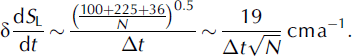
Typically N ranges from <10 in sparsely surveyed areas to many tens in areas where there are many surveys, primarily in the north of the Greenland ice sheet. The time interval, Δt, is typically 5 years. Consequently δdS L/dt ranges from a maximum of ∼1 cm a−1 for sparsely surveyed grids, mainly in the south, to 0.4 cm a−1 for well-surveyed grids in the north.
Radar
The ERS-derived estimates of elevation-change rates (dS R/dt) were obtained by fitting a straight line to elevation time series at ‘clusters’ of nearly co-located orbit crossing points, with errors (ε) determined by differences between the line and the data. This includes both observation errors and seasonal variability. Then, with N clusters in a grid square:
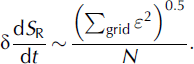
Typically, ε ∼ 10–30 cm a−1, and N increases from 2 in the south to >20 in the north, yielding δdS R/dt ranging from a worst case of ∼20 cm a−1 for a few grids in the south to <1 cm a−1 for a few grids in the north.
Interpolation
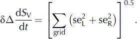
In addition to measurement errors, there are also errors resulting from the spatial variability of dS/dt within a grid square, and this can be large in regions of poor data coverage, particularly at lower elevations. The standard error (seL and seR) of the average laser and radar elevation-change estimate for each grid is a measure of this spatial variability. Consequently, we derive uncertainty estimates associated with spatial variability within a grid square as:
Errors on difference between estimates of dS/dt
The difference between the radar and laser estimates of dS/dt for a grid square is:
with errors:
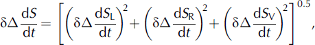
which, for ΔdS/dt estimates averaged over a region containing many (M) grids, becomes:

where M increases from <10 for lower-elevation averages in the south of the ice sheet to >100 for higher-elevation averages in the north.
This does not include the effects of errors that cause a systematic bias between ATM and GLAS measurements: a possible range bias between ATM and GLAS, including effects of trajectory errors, of <2 cm (Reference Martin, Thomas, Krabill and ManizadeMartin and others, 2005); and a possible bias (assumed to be <3 cm) in corrections applied for saturation of GLAS waveforms over ice. The associated ATM/GLAS bias results in a possible additional error of dS L/dt ∼ 7 mm a−1,which has been included in the uncertainty estimates listed in Table 2.
The estimates of ΔdS/dt shown in Figures 5 and 6 are averages of three sets of comparisons, so the uncertainties shown were calculated as the rms of the three uncertainty estimates.
We might expect a bias between radar and laser measurements because of the large difference in footprint sizes, with ERS providing an indication of average dS/dt over its pulse-limited footprint (∼1 km diameter), but such a bias should be small over higher-elevation parts of the ice sheet.
There are also errors associated with the interpretation of the radar and laser estimates of dS/dt, which are generally assumed to represent rates of elevation change. Laser-derived surface elevations have been well validated against other observations, so we interpret differences between the ATM/GLAS and the SRALT estimates of dS/dt as indicating errors in the SRALT estimates.


