


1. INTRODUCTION
Classifications of ice bodies are typically organized by size, geometry and dynamics. Barely flowing glacierets are exceedingly small (<1 km2) and radially flowing continental ice sheets are large (on the order of 106 km2). In between these two extremes are a cornucopia of ice caps, ice fields, glacier complexes, piedmont glaciers, valley glaciers, cirque glaciers and a host of other semantic designations; all of these are less aptly described by size alone than by important differences in geometry and dynamics (Cogley and others, Reference Cogley2011). Valley glaciers, for example, are delineated by well-defined lateral boundaries, determined by the surrounding mountain topography, across which there is no flow. Ice caps, on the other hand, are dome-shaped bodies that largely subsume the underlying bedrock topography and have flow patterns that are independent of, or significantly less influenced, by that topography.
Two different scales of ice thickness distinguish glaciers and ice caps. Let h be the characteristic or average thickness of an ice body. If h* is the characteristic vertical relief of the surrounding bedrock topography, then glaciers exist when h ≪ h* and ice caps exist when h ≫ h*. In between these extremes is a region dominated by glacier complexes and ice fields. As h → h*, the interaction between ice and the constraining bedrock leads to hybrid morphologies and dynamics that have some characteristics of both glaciers and ice caps.
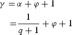
However, the distinctions between h ≪ h*, h → h* and h ≫ h* are more than taxonomic, and they delineate behaviors with practical ramifications. The volume/area scaling exponent γ, for example, is different for valley glaciers and ice caps (Lüthi, Reference Lüthi2009; Bahr and others, Reference Bahr, Pfeffer and Kaser2015). For ice volume V and the map-plane surface area S,
 $$V \propto {S^\gamma}. $$
with
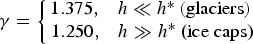 $$\gamma = \left\{ {\matrix{\!{{\rm 1}{\rm. 375,}\quad h \ll h{^\ast}\,{\rm (glaciers)}} \cr {{\rm 1}{\rm. 250,}\quad h \gg h{^\ast}\hbox{ (ice caps)}} \cr}} \right.$$
where γ = 11/8 = 1.375 and γ = 5/4 = 1.25 are selected from the theoretical developments of Bahr and others (Reference Bahr, Pfeffer and Kaser2015), and a multiplicative scaling parameter (unnecessary to the current development) can be defined as in Bahr and others (Reference Bahr, Pfeffer and Kaser2015) or Lüthi (Reference Lüthi2009). All the sea level rise studies that calculate volume based on surface area using Eqn (1) have to decide to which class each and every relevant ice body belongs. Small differences in γ can lead to significant differences in total volume and estimated sea level rise (e.g. Van de Wal and Wild, Reference Van de Wal and Wild2001; Meier and others, Reference Meier2007; Bahr and others, Reference Bahr, Dyurgerov and Meier2009; Leclercq and others, Reference Leclercq, Oerlemans and Cogley2011; Radić and Hock, Reference Radić and Hock2011; Slangen and van de Wal, Reference Slangen and van de Wal2011; Marzeion and others, Reference Marzeion, Jarosch and Hofer2012; Mernild and others, Reference Mernild, Lipscomb, Bahr, Radić and Zemp2013; Radić and Hock, Reference Radić and Hock2014). Deciding in which group to place glacier complexes and ice fields is particularly problematic, because they are often quite large, and these taxonomic oddities can thus have a potentially significant influence on total ice volume and consequent sea level rise estimates (Grinsted, Reference Grinsted2013).
The volume/area scaling exponent γ (as well as other scaling exponents), might be expected to have a range of size-dependent values between γ = 1.375 (small glaciers) and γ = 1.25 (large ice caps) with ice fields and glacier complexes occupying a range of intermediate values. Large, complexly branching, ice masses such as the Bering-Malaspina-Hubbard complex in Alaska or the Patagonia Ice Fields in Chile and Argentina might have intermediate geometries that are neither wholly glacier nor wholly ice cap.
While possible, we posit that a continuum of exponent values is unlikely for more than a very small collection of ice masses. No evidence or analysis has found a continuum of values, suggesting that the exponent γ shifts from the observationally supported values of 1.375 to 1.25 almost as a discontinuous step function, presumably varying as a function of h/h* (Eqn (2)). Abrupt transitions like this are not uncommon in nature and similar to other physical processes (e.g. Ma, Reference Ma1976; Dodds and Rothman, Reference Dodds and Rothman2000), we show how such an abrupt transition may arise and that a smoothly varying range of intermediate exponents and behaviors is unlikely. A classic non-thermodynamic example of an abrupt phase transition is fluid conductivity as a function of porosity (e.g. Stauffer and Aharony, Reference Stauffer and Aharony1992). As the porosity ρ varies smoothly from 0 to 1, the conductivity makes an abrupt transition at some critical value ρ c . For ρ ≪ ρ c there is no fluid conductivity, yet for ρ ≫ ρ c the fluid conducts freely. As ρ → ρ c, the fluid conductivity undergoes an abrupt transition. The mathematics of percolation theory can be used to describe the abrupt phase transition in fluid conductivity, and in an analogous manner we will use percolation theory to describe the abrupt transition from glaciers to ice caps.
To avoid confusion with thermodynamic phase transitions, we will refer to the abrupt changes in glacier geometry discussed here as ‘crossover phenomena’ and ‘crossover behaviors.’ The crossover is understood to be an abrupt change in some property as a function of another parameter. In a later section we will identify this parameter (sometimes called an order parameter) as the percentage of ice, ν, covering a particular mountain range, region or other designated topography. Other properties such as the width, length or thickness of an ice body will change abruptly as a function of ν, similar to the phase transition in fluid conductivity as a function of porosity as described above. The crossover can be a continuous function with discontinuous derivatives such as |ν c − ν|−k , as seen for example, with heat capacities and |T c − T|−k near the critical temperature T c.
We do not attempt an exhaustive list of crossover behaviors for all possible exponents. Instead we demonstrate the existence of crossover behaviors for several geometric parameters, and then demonstrate the consequent existence of similarly abrupt crossovers (as a function of h/h*) in a wide variety of glacier scaling exponents such as γ. The functional form of the crossover in the volume/area relation is not ascertained (except in a special one-dimensional (1-D) case), but neither is it necessary. The existence of an abrupt crossover is enough to establish that vanishingly few, if any collections of glaciers will have scaling exponents intermediate between glaciers and ice caps. (Bahr and others (Reference Bahr, Pfeffer and Kaser2015) discuss why scaling relationships and exponents are derived and observed for ensembles of glaciers rather than individual glaciers; throughout this text, we will always mean that the scaling exponents have been derived from ensembles, and any reference to ‘few if any’ glaciers will mean insufficient for an ensemble collection.) We do, however, offer a generic functional form for the crossover, and show that the generic function will be a power law, consistent with a wide variety of other crossover phenomena in statistical physics. For this reason, throughout the text, when we refer to a ‘rapid’ or ‘abrupt’ crossover, we take this to mean a divergent function, presumably a power law as seen in most analogous phase transitions such as those observed in fluid conductivity and heat capacity. In the following, a small variation in either h/h* or ν at or near a critical value will lead to the abrupt (power law) crossover.
Although the two endmember cases of γ = 11/8 = 1.375 for glaciers and γ = 5/4 = 1.25 for ice caps has been adequately addressed elsewhere with both theory (e.g. Lüthi, Reference Lüthi2009; Bahr and others, Reference Bahr, Pfeffer and Kaser2015) and data (e.g. Paterson, Reference Paterson1972; Chizhov and Kotlyakov, Reference Chizhov and Kotlyakov1983; Macheret and others, Reference Macheret, Cherkasov and Bobrova1988; Zhuravlev, Reference Zhuravlev and Avsyuk1988; Chen and Ohmura, Reference Chen and Ohmura1990; Grinsted, Reference Grinsted2013; Bahr and others, Reference Bahr, Pfeffer and Kaser2015), there has been little to no theoretical discussion of other values for other exponents that may fall in between. This paper addresses that specific gap by using percolation theory to mathematically model the rapid transition between the two endmembers.
Percolation theory is used quite commonly to describe the behavior of many different types of phase transitions (e.g. Stauffer and Aharony, Reference Stauffer and Aharony1992) and in particular to describe geometric and topographic-related transitions (e.g. Isichenko, Reference Isichenko1992). Our model follows in that rich tradition. However, we do not expect our work to be the final word in the analysis of glacier and ice cap geometries, in part because our result is pseudo 2-D and in part because many other statistical physics approaches are possible. Just as the flow of a glacier can be described using many different theoretical approaches such as continuum mechanics, statistical mechanics and cellular automata, we fully expect that there are other equally valid models of the glacier to ice cap geometric phase transition; a traditional phase change model borrowed from statistical mechanics is certainly one possibility (c.f. Ma, Reference Ma1976). Nevertheless, as a first attempt to fill a theoretical gap, our percolation model is sufficient to validate the existence of an abrupt transition in the volume/area scaling exponent as h/h* → 1. As such, the following analysis provides some theoretical justification for practitioners who want to assign either an ice cap scaling exponent or a glacier scaling exponent without the need to consider other rare or non-existent intermediate values.
2. HISTORICAL PERSPECTIVE
In many respects, the nearly discontinuous transition in parameter values from a ‘glacier’ to an ‘ice cap’ is an intuitive consequence of distinct differences understood to exist between these objects: their geometry is classified as linear versus radial, and their flow regime is constrained versus unconstrained. Less obvious is whether physics will support a continuum of geometries between these endmembers.
Theoretical scaling arguments (e.g. Lüthi, Reference Lüthi2009; Bahr and others, Reference Bahr, Pfeffer and Kaser2015) and volume/area data (e.g. Paterson, Reference Paterson1972; Chizhov and Kotlyakov, Reference Chizhov and Kotlyakov1983; Macheret and others, Reference Macheret, Cherkasov and Bobrova1988; Zhuravlev, Reference Zhuravlev and Avsyuk1988; Chen and Ohmura, Reference Chen and Ohmura1990; Grinsted, Reference Grinsted2013) suggest that glaciers and ice caps are in fact distinct. Data are sparse, however, with hundreds of volume/area measurements compared with hundreds of thousands of glaciers and ice caps. Theoretical considerations aside, it has been unclear to some practitioners whether additional volume, area and thickness measurements will reveal exceptions to the widely used scaling exponents. Noisy data compound the uncertainties (Farinotti and Huss, Reference Farinotti and Huss2013; Grinsted, Reference Grinsted2013), as do occasional questions about data integrity (Haeberli and others, Reference Haeberli, Hoelzle, Paul and Zemp2007; Lüthi and others, Reference Lüthi, Funk and Bauder2008) and differences (and similarities) between data and modeling results (Pfeffer and others, Reference Pfeffer, Sassolas, Bahr and Meier1998; Adhikari and Marshall, Reference Adhikari and Marshall2012). However, in a general sense most of the uncertainties have revolved around finding appropriate values for the volume/area exponent of glaciers, rather than finding an appropriate exponent for ice caps. For ice caps, a simple, intuitive geometric argument is widely accepted as a justification for γ = 1.25 (e.g. Lüthi, Reference Lüthi2009; Cuffey and Paterson, Reference Cuffey and Paterson2010; Radić and Hock, Reference Radić and Hock2010; Bahr and others, Reference Bahr, Pfeffer and Kaser2015).
For glaciers, we will use the theoretically derived value of γ = 11/8 = 1.375. For the purposes of this paper, however, the exact value is not nearly as important as its distinction from the ice cap value of γ = 5/4 = 1.25, and we could (in the context of this paper) alternatively select a glacier value of γ = 7/5 = 1.4 from the theoretical developments of Lüthi (Reference Lüthi2009) (Lüthi's is slightly different but generally consistent value is derived with an assumption of infinite glacier widths). Regardless of the value, the specific behavior as h → h* remains unknown and only the endmember cases are established by previous theoretical developments (Lüthi, Reference Lüthi2009; Bahr and others, Reference Bahr, Pfeffer and Kaser2015). Typically, Eqn (2) is treated as a step function that jumps discontinuously from 1.375 for glaciers to 1.25 for ice caps.
Data for the characteristic glacier width w and length l also show a split in scaled values (Bahr, Reference Bahr1997a). The characteristic glacier width is typically defined as the average width in the along-flow direction (e.g. Bahr, Reference Bahr1997a), though it can also be defined as the width at a specific elevation as pointed out in the discussion of characteristic values by Bahr and others (Reference Bahr, Pfeffer and Kaser2015). The characteristic length is typically defined as the along-flow curvilinear length from the highest to the lowest elevations of a glacier, but other possible characteristic values include the semi-major axis of the smallest ellipse encompassing the glacier or other lengths as discussed by Bahr and others (Reference Bahr, Pfeffer and Kaser2015). For the typical characteristic values of average width and curvilinear length, extensive data in Bahr (Reference Bahr1997a) show that
 $$w = {c_{\rm w}}{l^{\rm q}}$$
for some scaling parameter c w and
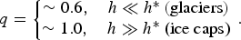 $$q = \left\{{\matrix{{\!\sim 0.6,\quad h \ll h{^\ast}\,{\rm (glaciers)}} \cr {\!\sim 1.0,\quad h \gg h{^\ast}\hbox{ (ice caps)}} \cr}} \right..$$
In addition to the width data, other accumulation/area ratio data and mass balance data also imply this same split in the exponent q (Bahr and others, Reference Bahr, Pfeffer and Kaser2015). The volume/area exponent γ can be derived as a function of q (Eqns (127) and (132) of Bahr and others, Reference Bahr, Pfeffer and Kaser2015), so the crossover suggested by Eqn (4) implies the crossover in Eqn (2).
Glacier area/length scaling is closely related to width/length scaling and is expected to show similar crossover behavior. Multiplying each side of Eqn (3) by the length l,
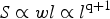 $$S \propto wl \propto {l^{{\rm q} + 1}}$$
and
 $$l \propto {S^\alpha} $$
where
 $$\alpha \equiv \displaystyle{1 \over {(q + 1)}}.$$
In fluvial geomorphology, Eqn (6) is called Hack's law (Hack, Reference Hack1957), and the exponent α has a typical value of 0.6 and a range of ~0.5–0.7 depending on the scale of the river basin. However, heuristic arguments for river drainage networks (Dodds and Rothman, Reference Dodds and Rothman2000) suggest that the Hack's law exponent α is expected to exhibit crossover phenomena as the river basin size increases from a regional channel-dominated landscape (α ≈ 0.6) to a largely unconstrained continental-scale landscape where α ≈ 1. Although the dynamics of water and ice are different, the Hack's law crossover behavior appears to be similar for both fluvial geomorphology and glaciology.
Many other geometric scaling relationships describe river drainage networks, such as basin width to basin area scaling and basin length to main channel length scaling (e.g. Horton, Reference Horton1945; Strahler, Reference Strahler1957; Peckham and Gupta, Reference Peckham and Gupta1999). The exponents of all these other geometric scaling relationships are simple polynomial ratios of two suitably selected scaling exponents, such as the Hack's law exponent and the exponent relating river basin length to main channel length (Dodds and Rothman, Reference Dodds and Rothman1999). As a result, any crossover behavior in Hack's law will lead to crossover phenomena in other fluvial scaling relationships. The reduction of all scaling exponents to just one or two other specific scaling exponents is a common feature of crossover phenomena in many disciplines such as statistical mechanics, thermodynamics and percolation theory (e.g. Ma, Reference Ma1976; Stauffer and Aharony, Reference Stauffer and Aharony1992). As with these other disciplines, rapid crossover phenomena are common and expected in fluvial geomorphology.
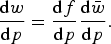
In a manner analogous to both thermodynamics and geomorphology, glacier scaling relationships for each of the major continuum mechanical variables (width, length, thickness, volume, area, velocities, stresses, time, mass balance, etc.) have exponents that can be defined in terms of two other scaling exponents γ and q. (Glen's flow law exponent n is also necessary, but this is a material constant that does not vary with any crossover phenomena.) For example, the characteristic along-flow velocity u scales with surface area as (Bahr, Reference Bahr1997b)
 $$u \propto {S^{(\gamma - 1)(2n + 1) - n/(q + 1)}}.$$
(As discussed by Bahr (Reference Bahr1997b) and Bahr and others (Reference Bahr, Pfeffer and Kaser2015), Eqn (8) is valid for large ensembles of glaciers; in an average sense, larger glaciers have higher surface velocities. Exceptions can be found for individual glaciers, but this is irrelevant to the ensemble scaling relationship.) Large glaciers are typically closer to the glacier/ice cap transition, and thus the derivation of Eqn (8) assumes that the surface slope scales as θ ∝ h/l, as is typical of large glaciers and ice caps.
More generally, in glaciology the characteristic values for any two geometric or dynamic continuum mechanics variables X and Ψ (characteristic values for those variables that appear in a standard continuum mechanical description of flow) scale as
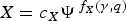 $$X = {c_X}{\Psi ^{{\,f_X}(\gamma, q)}}$$
where f X is a simple quotient of two polynomials (Bahr, Reference Bahr1997b). Equation (9) is an important relationship for this paper because it allows us to define and combine a variety of scaling relationships that will connect glacier widths to thickness and volume. Moreover, if rapid crossover phenomena are observed for width/length scaling (exponent q) and/or volume/area scaling (exponent γ) then Eqn (9) shows that crossover phenomena are expected to be ubiquitous throughout glacier geometry and continuum mechanical variables X and Ψ.
There is nothing unique about the choice of q and γ in Eqn (9), and we could just as easily use many other exponent combinations such as γ and Hack's law exponent α. The choice of q and γ is largely historical, motivated by available datasets for width/length and volume/area. Table 1 provides examples, including scaling that is based on the slope/area scaling exponent φ (substitute slope and area into Eqn (9)) and Hack's law exponent α. This leads to
 $$\eqalign{\gamma =\, & \alpha + \varphi + 1 \cr = & \displaystyle{1 \over {q + 1}} + \varphi + 1} $$
which explicitly shows the relationship between the volume/area exponent γ and the width scaling exponent q (c.f. Eqns (127) and (132) of Bahr and others, Reference Bahr, Pfeffer and Kaser2015). This will be especially useful when showing that a crossover in width scaling is related to a crossover in volume scaling.
Table 1. Power law scaling exponents for relationships of the form X ∝ Ψ f X (γ,q) and X ∝ Ψ f X (α,φ) where all scaling parameters X and Ψ are characteristic values

Exponents are closely related to each other, and crossover phenomena in γ and q (or α and φ) will lead to crossover phenomena for all the other relationships as well. (Slope is an exception for the specified values of q and λ; such degenerate cases are permitted by the analysis in this paper.) Specific values are listed for glaciers (γ = 1.375, q = 0.6, n = 3) and ice caps (γ = 1.25, q = 1, n = 3). Note that n is a material constant and is not a scaling exponent. An exponent of 0 indicates that the parameter scales as a constant with respect to Ψ. For example, the characteristic mass balance rate
 $\dot b$
of ice caps scales as a constant with respect to size, as intuited and assumed in ice sheet scaling analyses by Vialov (Reference Vialov1958), Weertman (Reference Weertman1961), Paterson (Reference Paterson1972), and others. Bahr (Reference Bahr1997b) provides additional details and derivations.
$\dot b$
of ice caps scales as a constant with respect to size, as intuited and assumed in ice sheet scaling analyses by Vialov (Reference Vialov1958), Weertman (Reference Weertman1961), Paterson (Reference Paterson1972), and others. Bahr (Reference Bahr1997b) provides additional details and derivations.
Data analysis for thousands of sub-basins of the Columbia, Knik, Russell, Harvard, Barnard and Matanuska glaciers (all in Alaska) show that Hack's exponent is α = 0.466, 0.481, 0.493, 0.497, 0.513 and 0.518, respectively (Bahr and Peckham, Reference Bahr and Peckham1996) (c.f. Table 1). Using q = (1/α) − 1 from Eqn (7), this corresponds to width/length scaling exponents (as derived from the data) of q = 1.15, 1.08, 1.03, 1.01, 0.95 and 0.93. Evidently, these very large many branched glacier complexes are behaving more like ice caps (q ≈ 1) than valley glaciers (q ≈ 0.6). Accordingly, we should posit that all of these glaciers have continuum properties (volume, thickness, velocities, stresses, etc.) that will scale like ice caps. Additional data are needed both to support such a conjecture and to generalize to other complex multi-branched glaciers, but the existence of volume/area and width/length crossover behaviors would make such a hypothesis reasonable.
The majority of theoretical developments in ice physics are rooted in continuum mechanics and thermodynamics (e.g. Cuffey and Paterson, Reference Cuffey and Paterson2010), but although less common, statistical physics has been successfully applied to iceberg calving (Bahr, Reference Bahr1995; Bassis, Reference Bassis2011; Åström and others, Reference Åström2013, Reference Åström2014) and crossover behaviors in the permeability of sea ice (Golden and others, Reference Golden, Ackley and Lytle1998). Other applications of statistical physics and their models include glacier sliding (Bahr and Rundle, Reference Bahr and Rundle1996; Fischer and Clarke, Reference Fischer and Clarke1997; Sergienko and others, Reference Sergienko, MacAyeal and Bindschadler2009; Åström and others, Reference Åström2013), visco-elastic glacier flow (Bahr and Rundle, Reference Bahr and Rundle1995; Åström and others, Reference Åström2013) and snowpatch size distribution (Bahr and Meier, Reference Bahr and Meier2000). Within most of these studies is a recurring power law scaling relationship with an exponential tail. This power law scaling is so common within statistical physics that it nearly deserves elevation to the status of ‘guiding principle’ or ‘law’ and reflects the disappearance of length scales near crossover phenomena (power law) and the re-emergence of length scales on either side of the crossover (exponential tail) (Stauffer and Aharony, Reference Stauffer and Aharony1992, pp. 64 and 151). A similar scaling relationship is reasonably expected and in fact will be derived for the glacier and ice cap crossover.
3. OUTLINE OF THE CROSSOVER SOLUTION
It will be seen that the crossover in the relationship between the volume and area of ice masses is ultimately derived from the intrinsic nature of the topography in which they exist. For a small glacier with h/h* ≪ 1 (i.e. ice thickness much less than the characteristic scale of the surrounding topography), the glacier width w is small compared with length and is constrained by the surrounding topography. If mass balance changes cause the glacier to grow thicker with time, then the width will also increase (except in the very unusual case of a valley with vertical side walls). If the glacier grows so large that h/h* → 1− (the negative indicating ‘from below’), then the ice will begin to flow over surrounding ridges and summits. At this point, different glaciers in adjacent valleys will start to merge, and the width is significantly less constrained. When h/h* ≫ 1, the width is completely unconstrained and scales identically to the length.
While the crossover from constrained to unconstrained lateral extent is easily visualized, the rate of crossover is not obvious. Given a specific topography for a specific mountain range, we could numerically model the growth of glaciers, observing how the width changes with the thickness scale h/h*. A more general approach would use generic rather than specific mountain ranges, perhaps utilizing Brownian noise topographies (e.g. Turcotte, Reference Turcotte1997). Better still, we can look at all possible mountain ranges simultaneously as an ensemble, using probabilities to guarantee that any and all topographies are expected to have the same w = f(h/h*) scaling behavior. By demonstrating a crossover on all possible topographies, we know that any real topography (the Himalaya, European Alps, Svalbard, Baffin Island, etc.) is included as a subset.
Although rooted in statistical physics, the ensemble approach is straightforward and starts with a 1-D transect across the surface of an arbitrary glacierized region (as shown in Fig. 1). Some parts of the transect are covered by glacier ice and other parts are not. Momentarily ignoring connections that might occur somewhere out of the plane of the transect, each ice patch on the transect is treated as a separate glacier or ice body.

Fig. 1. A transect (or vertical cross section) perpendicular to the ice flow direction and parallel to the spine of a mountain range. The transect is offset from the spine by some arbitrary distance. Glaciers flow downhill so ice will tend to fill valley bottoms, but this is not a requirement of our analysis. For the separate ice bodies shown in this figure, valley side walls constrain the dynamics, and as outlined by Bahr and others (Reference Bahr, Pfeffer and Kaser2015), Lüthi (Reference Lüthi2009) and other theoretical works, the volume/area scaling exponent will be 1.375 (or 1.4 in Lüthi, Reference Lüthi2009). However, if the ice in this region grows thicker, the individual valleys are overtopped, and the separate ice bodies will eventually merge, covering the entire range. Consequently, the separate glaciers will have merged into an ice cap with radial flow that is significantly less constrained by the underlying topography, and as outlined in the referenced theories, the volume/area scaling exponent will be 1.25. Note also the illustration in Figure 2.
Using probabilities, the average size or ‘width’ of all of the ice patches (i.e. ice bodies or glaciers) is calculated. As the percentage of ice on the transect increases, the mean width of the glaciers also increases. Although restricted to 1-D, these initial results will be exact and show that the width grows rapidly as a power law (with respect to the percentage of ice on the transect). At the critical point of rapid growth (effectively a divergence), a set of many small glaciers abruptly crosses over to a single large ice cap that spans the entire transect. The specifics of this simplified 1-D solution will differ from the final result, but this case captures the essence of the generalized solution and makes the overall presentation clearer.
The solution is then extended to a pseudo 2-D map-plane surface by considering the connections that occur out of the plane of the original transect. For example, the transect might cross two branches of the same glacier that connect at a downstream confluence. We retain the original transect, but we now calculate the distances (along the transect) over which separate ice patches on the transect are actually connected at downstream confluences (if they are connected at all). This connectivity (which in this pseudo 2-D solution remains the correlation length as in the 1-D case) is calculated as a function of ice patch size – larger patches are part of bigger and longer glaciers that can reach further and are more likely to connect with other ice patches at some distant (or nearby) confluence. As the amount of ice on the map-plane surface increases, the connection (and correlation) length grows rapidly and effectively diverges. In this case, the divergence is even more rapid than the 1-D calculation and happens when a smaller percentage of ice covers the map-plane surface. At the point of divergence, a collection of small separate glaciers suddenly coalesces into one large ice cap.
4. WIDTH CROSSOVER ON A TRANSECT
Consider a transect (or 2-D vertical cross section) through a glacierized mountain range. Some parts of this transect are covered in ice, and other parts such as high ridges, nunataks and peaks are not covered in ice. Throughout the text, a ‘length scale’ can be understood to be in any orientation and may refer to a glacier width, thickness or length in the flow direction. For simplicity we will use transects that are dominantly parallel to and at some down-flow arbitrary distance from the flow-divide or spine of a mountain range (Fig. 1); the associated length scales in this transect are thus glacier widths. Alternatively, if the transect is perpendicular to the ridgeline, then the length scale along the transect is a measure of glacier length in the along-flow down-slope direction. Other transects have other (and perhaps less useful) length scales at arbitrary angles to the mean flow direction. Although unnecessary, all of the following results could be generalized for arbitrarily-oriented transects.
Let ν be the percentage of a given transect that is covered in ice. Then p = ν/100 is the probability that a randomly selected point on the transect will be covered in ice. When p = 0, none of the range is covered in ice. When p = 1, the entire range is subsumed by a single ice cap. When 0 < p < 1, a fraction p of the transect is covered in ice and contains some number N of distinct ice patches. For simplicity, we will refer to these N taxonomically uncategorized ice patches as generic ‘ice bodies’, and these could range from glacierets to glaciers to glacier complexes to ice fields; by definition, however, these unclassified ice bodies cannot be ice caps until they have subsumed the topography (Fig. 2).

Fig. 2. A vertical cross section with some percentage ν of the bedrock covered in ice. Dashed lines show ν = 0 (no ice), 0 < ν < 100 (some number of distinct ice bodies) and ν = 100 (a single ice cap).
By discretizing the transect into intervals of width Δx (Fig. 3), we can fill each interval with ice with probability p. The randomly occupied intervals represent one possible distribution of ice on the landscape, which we will refer to as a landscape realization R. As Δx → 0, all possible landscapes with a percentage of ice, ν can be generated in this manner. If for each discretization interval we were to represent ice covered areas with a 1 and ice free areas with a 0, then a binary string such as
 $$R = 01111111101110000001000001100$$
would represent the distribution of ice along the transect (Fig. 3). In this realization, 14 out of 29 intervals are filled with glacier ice, so p ≈ 14/29 = 0.48 and there are four distinct glaciers with widths of 8Δx, 3Δx, 1Δx and 2Δx.

Fig. 3. Two possible bedrock elevation profiles (solid curve and short dashed curve) for the arrangement of ice indicated by the landscape realization R = 01111111101110000001000001100. An infinite number of topographies can be associated with each R.
For every topography and associated transect with discretization interval Δx, there exists a unique realization R. On the other hand, for every R, there are an infinite number of corresponding non-unique topographies (Fig. 3). For example, the zeroes in R = 01111111101110000001000001100 could represent small ridges standing barely above the ice, or they could represent high summits. However, this is irrelevant to our analysis of glacier widths as a function of p, and as p increases (or decreases) by a small amount Δp, the number of 1s in the string R increases (or decreases), and the average widths of the randomly generated ice bodies (represented by consecutive strings of 1s) will also increase (or decrease). To change the average width, the corresponding ice thickness will compensate as necessary (Eqn (9); larger glaciers tend to be thicker); the thickness might change by a small amount if the zeroes represent ridges that are barely higher than the glacier, or the thickness might change dramatically if the zeroes represent high peaks. Either way, the thickness does not alter the behavior of the width as a function of p. The thickness is simply responding as a function of p and the width; this relationship between thickness and width will connect the percolation analysis to the behavior of h/h* → 1.
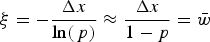
Reducing the distribution of ice to a 1-D binary string allows us to use well-established arguments from 1-D percolation theory (e.g. Stauffer and Aharony, Reference Stauffer and Aharony1992). In particular we can calculate the average width of each ice body, or equivalently the average size of each cluster of adjacent 1s. In Figure 3, the average is (8 + 3 + 1 + 2) Δx/4 = 3.5 Δx. More generally, for an arbitrary R, the probability that an interval Δx is occupied by ice is p. The probability that m adjacent intervals are occupied by ice is pm . Note, however, that to form an ice body made up of m intervals (and not larger), the occupied intervals (marked by 1s) would need to be surrounded on each end by unoccupied intervals (marked by 0s). The probability that an interval Δx is not occupied by ice is 1 − p. Therefore, the probability that an ice body on R has width m Δx will be (1 − p)p m (1 − p). If w* is the total width of the transect and M = w*/Δx is the total number of intervals in the transect, then we expect that the total number of ice bodies of width m Δx will be
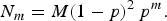 $${N_m} = M{(1 - p)^2}{\,p^m}.$$
This assumes that Δx → 0 and M → ∞ so that we can ignore the effects of the end points on our finite-length transect.
From Eqn (12), the total number of all ice bodies is
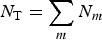 $${N_{\rm T}} = \sum\limits_m {{N_m}} $$
where m runs from 1 to ∞ both here and in all subsequent summations. Also from Eqn (12), m Δx N m is the total aggregate width of all the ice bodies that happen to have the exact width of m Δx. Therefore the total width w T of all ice bodies of any width is
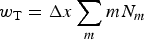 $${w_{\rm T}} = \Delta x\sum\limits_m {m{N_m}} $$
and the average width of all ice bodies is
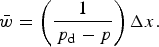
 $$\displaylines{\bar w = \displaystyle{{{w_{\rm T}}} \over {{N_{\rm T}}}} \cr = \displaystyle{{\sum\limits_m {m{N_m}}} \over {\sum\limits_m {{N_m}}}} \Delta x \cr = \displaystyle{{\sum\limits_m {m{p^m}}} \over {\sum\limits_m {{\,p^m}}}} \Delta x} $$
where the denominator of the final equality is a geometric series (with m = 1 to ∞) and reduces to p/(1 − p). The numerator also reduces to a geometric series,
 $$\eqalign{\sum\limits_m {m{p^m}} & = \sum\limits_m {\,p\displaystyle{{{\rm d}({\,p^m})} \over {{\rm d}p}}} \cr & = p\displaystyle{{\rm d} \over {{\rm d}p}}\left( {\sum\limits_m {{\,p^m}}} \right) \cr & = p\displaystyle{{\rm d} \over {{\rm d}p}}\left( {\displaystyle{\,p \over {1 - p}}} \right) \cr & = \displaystyle{\,p \over {{{(1 - p)}^2}}}.} $$
Therefore, from Eqns (15) and (16), the average width of all glaciers on the transect R is
 $$\bar w = \left( {\displaystyle{1 \over {1 - p}}} \right)\Delta x.$$
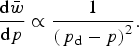
We are interested in the divergence of the width, and in particular the rate at which the width crosses over from separate ice masses to a single large ice cap that spans all of R. The presence of any 0 within R indicates bedrock, and therefore the crossover to a single ice cap spanning all of R can only happen when p = 1. This is referred to as the critical threshold p c, and
 $${\,p_{\rm c}} = 1.$$
Later in our 2-D solution, the critical threshold will drop to a more useful value that is <1 so that the threshold can be approached from both above and below. For now, as
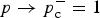 $p \to p_{\rm c}^ - = 1$
from below, Eqn (17) indicates that the width diverges at a rate given by
$p \to p_{\rm c}^ - = 1$
from below, Eqn (17) indicates that the width diverges at a rate given by
 $$\displaystyle{{{\rm d}\bar w} \over {{\rm d}p}} \propto \displaystyle{1 \over {{{(1 - p)}^2}}}.$$
when p ≪ p
c, the rate is close to 1. On the other hand, as
 $p \to p_{\rm c}^ - $
, the rate
$p \to p_{\rm c}^ - $
, the rate
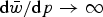 ${\rm d}\bar w/{\rm d}p \to \infty $
, indicating a very sudden crossover phenomena from glaciers to ice caps. The crossover occurs both as
${\rm d}\bar w/{\rm d}p \to \infty $
, indicating a very sudden crossover phenomena from glaciers to ice caps. The crossover occurs both as
 $p \to p_{\rm c}^ - $
and as
$p \to p_{\rm c}^ - $
and as
 $\bar w \to w^*$
.
$\bar w \to w^*$
.
5. GENERALIZATION TO A MAP-PLANE PROJECTION
Expanding this theory from its application to features along a 1-D transect across topography to the relationships between features in a 2-D topography is non-trivial and requires careful analysis. A large, complexly dendritic glacier (the Columbia Glacier, in coastal Alaska, is a good example) may have many branches and a high Strahler stream order (Horton, Reference Horton1945; Strahler, Reference Strahler1957; Bahr and Peckham, Reference Bahr and Peckham1996); if a transect (or vertical cross section) R is just barely upstream of the confluence between two branches, then the connected ice body will intersect the transect R in two separate locations. What looks like two separate glaciers on the transect is therefore actually one glacier, connected at an out-of-transect confluence.
For such a branched glacier, the width along a transect R is no longer the best (or the unique) measure of the actual glacier width. Instead, we need an effective glacier width that indicates the distance at which apparently separate ice bodies are actually connected by a confluence that exists somewhere off the transect. Because of these out-of-plane connections, the average of the effective width will be larger than the previously derived average width
 $\bar w$
and will diverge at some p
c < 1. In this case, we can model the width's crossover behavior as we approach it from both below and above.
$\bar w$
and will diverge at some p
c < 1. In this case, we can model the width's crossover behavior as we approach it from both below and above.
Suppose two randomly selected ice bodies on the transect R are separated by a distance d (Fig. 4). These bodies may or may not be separate glaciers, i.e. they may or may not connect at a downstream confluence, but a confluence may exist in the underlying bedrock topography regardless of whether or not the ice bodies encountered on the transect extend all the way to that point. For all randomly selected pairs of ice bodies, let the average distance between them be
 $\bar d$
. The average distance
$\bar d$
. The average distance
 ${\bar d_{\rm c}}$
to the nearest mutual confluence will be an increasing function of
${\bar d_{\rm c}}$
to the nearest mutual confluence will be an increasing function of
 $\bar d$
. Call this increasing function f
c. Generally, the confluence linking nearby ice bodies (glacier tributaries) will also be nearby. Widely separated ice bodies (tributaries) will have a confluence that is further away. Any other arrangement would violate fundamental topological constraints.
$\bar d$
. Call this increasing function f
c. Generally, the confluence linking nearby ice bodies (glacier tributaries) will also be nearby. Widely separated ice bodies (tributaries) will have a confluence that is further away. Any other arrangement would violate fundamental topological constraints.

Fig. 4. A stylized map-plane view of a glacier with two branches intersected by a transect (dashed line). The distance between the two intersections (ice patches on the transect) is d. The distance to the confluence can be different for each branch (d
c1 and d
c2), so we arbitrarily choose the average and set d
c = (d
c1 + d
c2)/2. The text uses average distances
 $\bar d$
and
$\bar d$
and
 ${\bar d_{\rm c}}$
over all pairs of ice patches.
${\bar d_{\rm c}}$
over all pairs of ice patches.
In fluvial geomorphology, most length parameters are related by power laws to other geometric quantities such as width and area (Peckham and Gupta, Reference Peckham and Gupta1999; Dodds and Rothman, Reference Dodds and Rothman2000). Hack's law is an example. Because glaciers sit in the same or similar landscapes as rivers, similar power laws may be expected to define the stream-length relationships of glaciers. (Using basin statistics, Bahr and Peckham (Reference Bahr and Peckham1996) have identified many such power laws for glaciers.) The function f
c relating
 $\bar d$
to
$\bar d$
to
 ${\bar d_{\rm c}}$
is reasonably expected to be a power law function of
${\bar d_{\rm c}}$
is reasonably expected to be a power law function of
 $\bar d$
:
$\bar d$
:
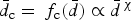 $${\bar d_{\rm c}} = {\,f_{\rm c}}(\bar d) \propto {\bar d^{\,\chi}} $$
for some scaling exponent χ>0. The first and more general relationship f c is the one we use in the following derivations. The second power law relationship in Eqn (20) is a reasonable hypothesis only and will be used to guide our intuition about the rate of divergence.
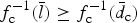
Consider two apparently separate ice bodies on the transect R. As p increases, the apparent width of each body on the transect increases in accordance with Eqn (17). As the width of each ice body increases, so does the length of that body in accordance with Eqn (3). The length of the body is not constrained to the transect because the ice flows downslope, regardless of whether or not this is in the direction of the transect. As the mean widths and lengths of the two ice bodies increase, they are more likely to join, forming a single glacier, at a downstream confluence whose distance from the transect is given by Eqn (20) (of course they could still join at a higher elevation, but the probability of a join increases with length).
Formally, we can combine Eqns (3), (17) and (20) to get the distance over which one ice body is expected to be connected to another on the transect. For simplicity, we recast Eqns (3) and (17) as w = f
wl(l) and
 $\bar w = {f_{\rm p}}(p)$
. We also note that because f
wl is an increasing function, the average characteristic width
$\bar w = {f_{\rm p}}(p)$
. We also note that because f
wl is an increasing function, the average characteristic width
 ${\bar w_c}$
of all the ice bodies that intersect the transect will be an increasing function f
l of the average characteristic length
${\bar w_c}$
of all the ice bodies that intersect the transect will be an increasing function f
l of the average characteristic length
 $\bar l$
. i.e.
$\bar l$
. i.e.
 ${\bar w_c} = {f_l}(\bar l)$
. Furthermore
${\bar w_c} = {f_l}(\bar l)$
. Furthermore
 ${\bar w_{\rm c}}$
is clearly an increasing function f
wc of the average width on the transect
${\bar w_{\rm c}}$
is clearly an increasing function f
wc of the average width on the transect
 $\bar w$
(on average, a glacier branch cannot get wider at the point where it crosses the transect while shrinking everywhere else). i.e.
$\bar w$
(on average, a glacier branch cannot get wider at the point where it crosses the transect while shrinking everywhere else). i.e.
 ${\bar w_{\rm c}} = {f_{\rm w}}(\bar w)$
. Therefore, combining the above functions,
${\bar w_{\rm c}} = {f_{\rm w}}(\bar w)$
. Therefore, combining the above functions,
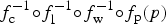
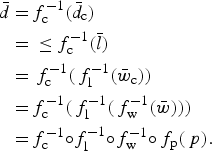 $$\eqalign{\bar d = \,& f_{\rm c}^{ - 1} ({{\bar d}_{\rm c}}) \cr = \,&\le f_{\rm c}^{ - 1} (\bar l) \cr = \,&\, f_{\rm c}^{ - 1} (\,f_{\rm l}^{ - 1} ({{\bar w}_{\rm c}})) \cr = \,& f_{\rm c}^{ - 1} (\,f_{\rm l}^{ - 1} (\,f_{\rm w}^{ - 1} (\bar w))) \cr = \,& f_{\rm c}^{ - 1} {\circ} f_{\rm l}^{ - 1} {\circ} f_{\rm w}^{ - 1} {\circ} {\,f_{\rm p}}(\,p).} $$
The inequality on the second line arises because
 $f_{\rm c}^{ - 1} $
is an increasing function and because connections between branches occur when the average length of the branch extends at least as far as the confluence, i.e. when
$f_{\rm c}^{ - 1} $
is an increasing function and because connections between branches occur when the average length of the branch extends at least as far as the confluence, i.e. when
 $\bar l$
is greater than or equal to the confluence distance
$\bar l$
is greater than or equal to the confluence distance
 ${\bar d_{\rm c}}$
. In other words,
${\bar d_{\rm c}}$
. In other words,
 $f_{\rm c}^{ - 1} (\bar l) \ge f_{\rm c}^{ - 1} ({\bar d_{\rm c}})$
when
$f_{\rm c}^{ - 1} (\bar l) \ge f_{\rm c}^{ - 1} ({\bar d_{\rm c}})$
when
 $\bar l \ge {\bar d_{\rm c}}$
.
$\bar l \ge {\bar d_{\rm c}}$
.
All the functions f
p,
 $f_{\rm w}^{ - 1} $
,
$f_{\rm w}^{ - 1} $
,
 $f_{\rm l}^{ - 1} $
and
$f_{\rm l}^{ - 1} $
and
 $f_{\rm c}^{ - 1} $
are monotonically increasing. Therefore,
$f_{\rm c}^{ - 1} $
are monotonically increasing. Therefore,
 $\bar d$
diverges as a function of p because f
p diverges as a function of p in Eqn (17). Furthermore, because each functional composition is monotonic,
$\bar d$
diverges as a function of p because f
p diverges as a function of p in Eqn (17). Furthermore, because each functional composition is monotonic,
 $f_{\rm c}^{ - 1} {\circ} f_{\rm l}^{ - 1} {\circ} f_{\rm w}^{ - 1} {\circ} {f_{\rm p}}(p)$
in Eqn (21) diverges at least as rapidly as the average width
$f_{\rm c}^{ - 1} {\circ} f_{\rm l}^{ - 1} {\circ} f_{\rm w}^{ - 1} {\circ} {f_{\rm p}}(p)$
in Eqn (21) diverges at least as rapidly as the average width
 $\bar w$
in Eqn (17).
$\bar w$
in Eqn (17).
Without further assumptions we cannot use Eqn (21) to establish a more precise rate of divergence. As a practical estimate, we can use the power law assumption in the second part of Eqn (20). We can also assume
 $\bar l = {f_{{\rm ld}}}({\bar d_{\rm c}})$
scales as a power law with some exponent λ>0 (as reasonably expected – see the previous heuristic argument regarding the power law relationships of geometric parameters in drainage networks). Then
$\bar l = {f_{{\rm ld}}}({\bar d_{\rm c}})$
scales as a power law with some exponent λ>0 (as reasonably expected – see the previous heuristic argument regarding the power law relationships of geometric parameters in drainage networks). Then
 $$\bar d = f_{\rm c}^{ - 1} {\circ} f_{{\rm ld}}^{ - 1} {\circ} f_{\rm l}^{ - 1} {\circ} f_{\rm w}^{ - 1} {\circ} {\,f_{\rm p}}(\,p) \propto {({\,p_{\rm c}} - p)^{ - \kappa}} \propto {(\bar w)^\kappa} $$
where κ = 1/(qχλ). Equation (22) is not essential for the development of the theory; but within the limitations of the built-in assumptions, Eqn (22) describes (very simply) the rate of divergence of
 $\bar d$
. We know a priori that
$\bar d$
. We know a priori that
 $\bar d \gt \bar w$
; therefore, κ > 1 and
$\bar d \gt \bar w$
; therefore, κ > 1 and
 $\bar d$
diverges much more rapidly than the average width
$\bar d$
diverges much more rapidly than the average width
 $\bar w$
. The crossover for
$\bar w$
. The crossover for
 $\bar w$
is rapid, so the crossover phenomenon for
$\bar w$
is rapid, so the crossover phenomenon for
 $\bar d$
is even more rapid.
$\bar d$
is even more rapid.
6. THE CORRELATION LENGTH AND CROSSOVER THRESHOLD
Let two randomly selected ice bodies be correlated if they are connected. As the distance between the bodies grows, both connections and correlations decrease. At distance r, the correlation function is typically defined as
 $$C(r) = {{\rm e}^{ - r/\xi}} $$
for some correlation length ξ.
Let two points on a transect R that are occupied by ice be separated by distance r. In the 1-D solution, these points are connected (correlated) if every interval Δx between them is also occupied by ice. If a single interval is occupied by ice with probability p, and the number of intervals is r/Δx, then the probability that two points on R are connected is
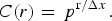 $$C(r) = {\,p^{{\rm r}/\Delta x}}.$$
By combining with Eqns (23) and (17), and using ln (p) ≈ p − 1 (valid for small p),
 $$\xi = - \displaystyle{{\Delta x} \over {\ln (\,p)}} \approx \displaystyle{{\Delta x} \over {1 - p}} = \bar w$$
The correlation length or connectivity length is the same as the average width of the glaciers (c.f. Stauffer and Aharony, Reference Stauffer and Aharony1992).
In the map-plane generalization, a correlation length can be defined radially in all directions, or we can instead define ξ
d as a new correlation length along the transect, indicating the new distances across which ice patches are connected on the transect. Clearly, for
 $r \lt \bar d$
, ice patches on the transect are likely to be connected, and for
$r \lt \bar d$
, ice patches on the transect are likely to be connected, and for
 $r \gt \bar d$
ice patches are less likely to be connected. In other words, the correlation length ξ
d is again proportional to the effective average width
$r \gt \bar d$
ice patches are less likely to be connected. In other words, the correlation length ξ
d is again proportional to the effective average width
 $\bar d$
. Using the assumed power law relationship between
$\bar d$
. Using the assumed power law relationship between
 $\bar w$
and
$\bar w$
and
 $\bar d$
in Eqn (22),
$\bar d$
in Eqn (22),
 $${\xi _{\rm d}} = \left( {\displaystyle{a \over {\Delta {x^{\kappa - 1}}}}} \right){\xi ^\kappa} $$
for some dimensionless constant a >0 and for a denominator that normalizes the units. As expected, the correlation length in the map-plane generalization is larger than the correlation length of the 1-D transect.
The critical threshold for the 1-D transect R is p c = 1. The critical crossover threshold in the map-plane generalization is
 $${\,p_{\rm d}} \lt {\,p_{\rm c}}.$$
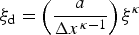
This crossover threshold p
d is reached when ξ
d is larger than any remaining bedrock span (i.e. clusters of adjacent 0s) on the landscape realization R. As with our analysis of average glacier widths (clusters of adjacent 1s), we can also estimate the average width of bedrock spans (clusters of 0s). The probability of an interval on R being free of ice (a ‘0’) is 1 − p. Generalizing from Eqn (17), the average bedrock width
 ${\bar w_b}$
is then
${\bar w_b}$
is then
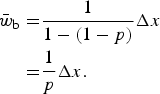 $$\eqalign{{{\bar w}_{\rm b}} = & \displaystyle{1 \over {1 - (1 - p)}}\Delta x \cr = & \displaystyle{1 \over p}\Delta x.} $$
The crossover phenomenon happens when p = p d and when the correlation length becomes
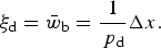 $${\xi _{\rm d}} = {\bar w_{\rm b}} = \displaystyle{1 \over {{\,p_{\rm d}}}}\Delta x.$$
Eqns (27), (28) and (29) are derived without assumptions.
With assumptions, we can push the derivation of p d further by substituting Eqns (26) and (17).
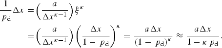 $$\eqalign{\displaystyle{1 \over {{\,p_{\rm d}}}}\Delta x = & \left( {\displaystyle{a \over {\Delta {x^{\kappa - 1}}}}} \right){\xi ^\kappa} \cr = & \left( {\displaystyle{a \over {\Delta {x^{\kappa - 1}}}}} \right){\left( {\displaystyle{{\Delta x} \over {1 - {\,p_{\rm d}}}}} \right)^\kappa} = \displaystyle{{a\Delta x} \over {{{\left( {1 - {\,p_{\rm d}}} \right)}^\kappa}}} \approx \displaystyle{{a\Delta x} \over {1 - \kappa {\,p_{\rm d}}}}.} $$
Solving for p d,
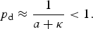 $${\,p_{\rm d}} \approx \displaystyle{1 \over {a + \kappa}} \lt 1.$$
Although their values are unknown, a >0 and κ >1. Therefore, the crossover threshold p d is smaller than 1, and as expected, p d < p c.
This final solution for the crossover threshold p
d depends on the reasonable but assumed power law relationship in Eqn (22). Nevertheless, it guides our intuition and suggests that (as expected) the crossover p
d can be approached from both above and below, unlike the less general p
c, which can only be approached from below. In other words, as
 $p \to {p_{\rm d}}^ \pm $
, the geometry will switch (as derived in Section 5) from a glacier to an ice cap and vice versa.
$p \to {p_{\rm d}}^ \pm $
, the geometry will switch (as derived in Section 5) from a glacier to an ice cap and vice versa.
7. THE RATE OF CROSSOVER
With p d < p c = 1, the probability that an interval Δx on the transect R is not occupied by ice is effectively reduced from 1 − p to p d − p. Equations (12)–(19) are adjusted in the expected manner. In particular, the number of glaciers of width m Δx in Eqn (12) changes to
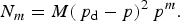 $${N_m} = M{({\,p_{\rm d}} - p)^2}{\,p^m}.$$
Substituting z ≡ |p d − p|m and ln p ≃ 1 − p, this has the promised power law exponential form (as a function of m) as seen repeatedly in the statistical physics of crossovers.
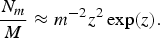 $$\displaystyle{{{N_m}} \over M} \approx {m^{ - 2}}{z^2}\exp (z).$$
Other than consistency with previous works, not too much should be read into this rather ad hoc transformation except that the exponential plays the role of a cutoff. For m ≪ 1/|p d − p| and m ≫ 1/|p d − p| there are two different regimes of behavior due to the exponential that depends on the average width, which is the generalized form of Eqn (17):
 $$\bar w = \left( {\displaystyle{1 \over {{\,p_{\rm d}} - p}}} \right)\Delta x.$$
For widths above and below the threshold, the behavior is that of glaciers and ice caps; but as
 $p \to p_{\rm d}^ \pm $
, the transition between the two is power law in form (and therefore rapid).
$p \to p_{\rm d}^ \pm $
, the transition between the two is power law in form (and therefore rapid).
As before, the most natural parameter for exploring the rate of transition is the average width of the glaciers or ice cap(s). This rate diverges near the threshold p d. Generalizing from Eqn (19) and directly from Eqn (34),
 $$\displaystyle{{{\rm d}\bar w} \over {{\rm d}p}} \propto \displaystyle{1 \over {{{({\,p_{\rm d}} - p)}^2}}}.$$
Far from the transition, this rate is roughly constant, and glacier and ice cap widths thus grow linearly. However, near the transition, as
 $p \to p_{\rm d}^ \pm $
, the rate is power law in form. For completeness, if Π ≡ p
d − p is a measure of the distance from the threshold, then the power law rate of divergence becomes explicit.
$p \to p_{\rm d}^ \pm $
, the rate is power law in form. For completeness, if Π ≡ p
d − p is a measure of the distance from the threshold, then the power law rate of divergence becomes explicit.
 $$\displaystyle{{{\rm d}\bar w} \over {{\rm d}\Pi}} \propto \displaystyle{1 \over {{\Pi ^2}}}.$$
The width scaling exponent q also diverges at a power law rate. As before, the characteristic widths in Eqn (3) are expected to grow as an increasing function f = f
wl°f
l of the average width
 $\bar w$
(see discussion of Eqn (21)). Therefore,
$\bar w$
(see discussion of Eqn (21)). Therefore,
 $$\displaystyle{{{\rm d}w} \over {{\rm d}p}} = \displaystyle{{{\rm d}f} \over {{\rm d}p}}\displaystyle{{{\rm d}\bar w} \over {{\rm d}p}}.$$
Similarly, the characteristic lengths grow as an increasing function of
 $\bar w$
, and
$\bar w$
, and
 $$\displaystyle{{{\rm d}l} \over {{\rm d}p}} \propto \displaystyle{{{\rm d}\bar w} \over {{\rm d}p}}.$$
Now consider large average (and large characteristic) widths and lengths, as is the case near the transition. Transforming Eqn (3), the width scaling exponent is
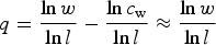 $$q = \displaystyle{{\ln w} \over {\ln l}} - \displaystyle{{\ln {c_{\rm w}}} \over {\ln l}} \approx \displaystyle{{\ln w} \over {\ln l}}$$
because ln(c w)/ln l is negligible for large l (note the discussion in Bahr and others (Reference Bahr, Pfeffer and Kaser2015) on the low order of multiplicative scaling parameters such as c w ), and q may thus be expressed as the first term only. Combining Eqns (37), (38) and (39), the rate of change of the scaling exponent is
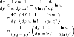 $$\eqalign{\displaystyle{{{\rm d}q} \over {{\rm d}p}} \propto & \displaystyle{1 \over w}\displaystyle{{{\rm d}w} \over {{\rm d}p}}\displaystyle{1 \over {\ln l}} - \displaystyle{1 \over {l{{(\ln l)}^2}}}\displaystyle{{{\rm d}l} \over {{\rm d}p}}\ln w \cr \propto & \displaystyle{{{\rm d}\bar w} \over {{\rm d}p}}\left( {\displaystyle{{{\rm d}f} \over {{\rm d}p}}\displaystyle{1 \over w}\displaystyle{1 \over {\ln l}} - \displaystyle{{\ln w} \over {l{{(\ln l)}^2}}}} \right) \cr \propto & \displaystyle{1 \over {{{({\,p_{\rm d}} - p)}^2}}}\left( {\displaystyle{{{\rm d}f} \over {{\rm d}p}}\displaystyle{1 \over w}\displaystyle{1 \over {\ln l}} - \displaystyle{{\ln w} \over {l{{(\ln l)}^2}}}} \right)} $$
where the important term is 1/(p d − p)2. For p near the crossover p d, the width/length scaling exponent q diverges rapidly as a power law. Away from the crossover, w and l remain large, and dw/dp is bounded and small so that dq/dp → 0. In other words, away from the threshold q behaves as a constant (which can differ on each side of the transition), as confirmed by observations in Eqn (4). Thus, Eqn (40) predicts the observed crossover in the width/length scaling exponent.
8. THE CROSSOVER FUNCTION
We can now write a very general relationship for the crossover behavior that depends on the percentage of ice relative to the critical threshold p d. From Eqn (40), q(p) resembles a step function between two constants; in the transition zone between the constants, dq/dp diverges, like the derivative of a step function. As noted in Eqn (9), a power law relates any two glaciological continuum parameters with scaling exponent f X(γ, q) or equivalently f X (α, φ) where α is the Hack's law exponent (Table 1). Therefore, Eqn (40) implies that the scaling exponents f X (γ, q) will split between two constants c 1 and c 2 (which in degenerate cases could be the same) depending on the relevant value of p. Values between c 1 and c 2 are possible, but rare due to the rapid crossover. The power law scaling exponent f X (γ, q) is therefore given by
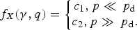 $${\,f_X}(\gamma, q) = \left\{{\!\matrix{ {{c_1},{\rm} p \ll {\,p_{\rm d}}} \cr {{c_2},{\rm} p \gg {\,p_{\rm d}}}. \cr}} \right.$$
When p ≪ p
d we have a glacier, and when p ≫ p
d we have an ice cap. Although conspicuously absent from Eqn (41), the intermediate behavior as
 $p \to p_{\rm d}^ \pm $
is implied as the rapid transition between c
1 and c
2; although almost straightforward enough to intuit, this deceptively simple equation is a direct consequence of Eqn (40).
$p \to p_{\rm d}^ \pm $
is implied as the rapid transition between c
1 and c
2; although almost straightforward enough to intuit, this deceptively simple equation is a direct consequence of Eqn (40).
Equation (41) shows that the crossover is sensitive to the percentage of the topography that is covered in ice. When comparatively little ice covers the landscape, we will have a set of separate valley glaciers; but when the percentage of ice covering the landscape exceeds some critical threshold, the ice will change abruptly from a set of separate valley glaciers to a single large ice cap. By definition, the thickness h → h*± as
 $p \to p_{\rm d}^ \pm $
, so more intuitively, the crossover is sensitive to the thickness of the ice relative to the ‘thickness’ (relative vertical relief) of the topography. In other words,
$p \to p_{\rm d}^ \pm $
, so more intuitively, the crossover is sensitive to the thickness of the ice relative to the ‘thickness’ (relative vertical relief) of the topography. In other words,
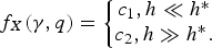 $${\,f_X}(\gamma, q) = \left\{{\!\matrix{ {{c_1},{\rm} h \ll h{^\ast}} \cr {{c_2},{\rm} h \gg h{^\ast}}. \cr}} \right.$$
When the geometry of an ice body is primarily defined by, and constrained by, the surrounding topography (h ≪ h*), the ice fits the definition of a glacier. When the ice grows thicker than the characteristic scale (relative vertical relief) of the surrounding topography (h ≫ h*), then the ice buries the landscape, and flows radially in all directions, independent of or significantly less constrained by the underlying landscape, fitting the definition of an ice cap.
Note that c 1 and c 2 differ for each power law relationship shown in Eqn (9), but their values are shown in Table 1 for a number of specific cases. Values in between c 1 and c 2 are unlikely to be encountered in nature because the transition is rapid; note Eqn (40), as well as the power law divergent behaviors of Eqns (34), (35) and, in a general sense, Eqns (19), (21) and (22). Equations (41) and (42) can thus be treated as step functions for most practical purposes. In particular, we do not expect the volume/area scaling exponent γ to have values between c 1 = 1.375 and c 2 = 1.25 except perhaps in vanishingly few instances. Noting that power law relationships apply to statistically large samples of glaciers, the presence of a very few exceptional cases need not be accounted for (Farinotti and Huss, Reference Farinotti and Huss2013; Bahr and others, Reference Bahr, Pfeffer and Kaser2015). Therefore, as a generally valid finding for volume/area scaling of glaciers, we have:
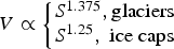 $$V \propto \left\{{\!\matrix{ {{S^{1.375}},{\rm glaciers}} \cr {{S^{1.25}}, \hbox{ ice caps}} \cr}} \right.$$
as explicitly derived from Eqns (9), (10) and (42). Note that the values of 1.375 and 1.25 are derived elsewhere (e.g. Lüthi, Reference Lüthi2009; Bahr and others, Reference Bahr, Pfeffer and Kaser2015), and the step between these values shown in Eqn (43) is a byproduct of the primary percolation analysis presented above.
9. CONCLUSIONS
The crossover in scaling properties from glaciers to ice caps (and vice versa) is highly sensitive to the thickness of the ice relative to the thickness of the topographic relief. As the mean ice thickness approaches the relative vertical relief of the topography, a very small change in thickness can trigger an abrupt step-function switch in the geometry of an ice body. There is very little room for ‘hybrid’ ice bodies that exhibit a geometry ‘in between’ a glacier and an ice cap. This is not meant to imply that such hybrid bodies do not exist, and examples are given in the introduction, but there will be very few of these bodies relative to the numbers of ice caps and glaciers. Notably, with the rapid non-linear crossover phenomena derived in Eqn (40), we expect insufficient ice bodies to generate ensemble statistics with volume/area scaling exponents that fall between 1.375 (for glaciers) and 1.25 (for ice caps). As implied by Table 1, Eqn (42) also shows that a wide variety of other scaling relationships will exhibit similarly rapid crossover behaviors.
Although simple in concept, the preceding analysis is perhaps inelegant in its mathematical complexity. Our expectation is that this analysis will be treated as a first step in the theoretical development of the transition between glacier and ice cap geometries. More elegant solutions using other statistical physics approaches may be possible. However, as it stands, the preceding theory strongly supports the notion that there are two primary volume/area scaling exponents, one for glaciers and one for ice caps. Other statistically valid exponents (generated from ensembles of glaciers) are unexpected, and this can be of significant value to practitioners who need to justify their choice of scaling exponents for sea level rise and other studies.
ACKNOWLEDGMENTS
We thank Martin Lüthi, Jo Jacka and two anonymous reviewers for helpful and thought provoking reviews and edits. We appreciate their willingness to dig into the mathematics. Publication was possible with generous support from the International Glaciological Society.


 Open access