


1. Introduction
The stability of parallel shear flows is well established in the fluid-mechanics community. The problem manifests both in the theoretical study of Kelvin–Helmholtz instabilities and in environmental and engineering flows. Blumen (Reference Blumen1970) studied the stability dynamics of a compressible shear flow with constant thermodynamic properties. In this regime, he showed that Fjørtoft's extension of Rayleigh's criterion, originally developed for incompressible shear layers, extends to the compressible flow regime. However, many engineering mixing flows involve binary and multispecies mixtures at trans- and supercritical conditions and thus feature complex thermodynamic response functions. The consideration of these effects is not covered by classical stability theory.
With increasing interest in high-pressure flow systems, much effort has been expended towards studying mixing flows at supercritical thermodynamic conditions. At these conditions, the fluids exhibit behaviours not found in subcritical conditions such as a sharp decrease in surface tension, resulting in diffused phase transition (Oschwald et al. Reference Oschwald, Smith, Branam, Hussong, Schik, Chehroudi and Talley2006). At the thermodynamic critical point, the saturation line, which delineates liquid and vapour regions at subcritical conditions, extends to the Widom line in the supercritical regime. It represents a degenerate form of phase transition between supercritical gas-like and supercritical liquid-like phases (Simeoni et al. Reference Simeoni, Bryk, Gorelli, Krisch, Ruocco, Santoro and Scopigno2010), see figure 1(a). Therefore, across the Widom line, transition from a liquid-like to a gas-like regime occurs, giving rise to large gradients in thermodynamic and transport properties. These enhanced variations in the thermodynamic response functions have been found to promote instabilities in Rayleigh–Bénard convection, swirling jet flows, channel flows and boundary layers (Accary et al. Reference Accary, Raspo, Bontoux and Zappoli2005; Ly, Rusak & Wang Reference Ly, Rusak and Wang2018; Ren, Fu & Pecnik Reference Ren, Fu and Pecnik2019a; Ren, Marxen & Pecnik Reference Ren, Marxen and Pecnik2019b). At increasing pressures, the distinction between supercritical gas-like and liquid-like phases diminishes, thus reducing the density variation across and lowering peak heat capacity at the Widom-line transition. In this regime, Zong et al. (Reference Zong, Meng, Hsieh and Yang2004) performed experimental investigations and conducted linear stability analysis (LSA) of supercritical single-species mixing flows of N $_{2}$. They concluded that at supercritical pressures, the dampening effect of the liquid–vapour interface is reduced and thus the single-species mixing layer becomes more unstable. Similarly, Roy & Segal (Reference Roy and Segal2010) performed experiments of N
 $_{2}$ injection at various sub/supercritical conditions and concluded that at supercritical conditions, the flow's density gradient reduced and that this behaviour strongly affects the length of the potential core.

Figure 1. (a) Thermodynamic regime diagram of CH $_{4}$/O
 $_{2}$ mixture at subcritical and supercritical conditions. Also plotted is the locus of thermodynamic conditions found in a representative isobaric baseflow. (b) Isobaric state space: isobaric projection of the supercritical thermodynamic regime diagram of CH
 $_{4}$/O
 $_{2}$ at
  $P=60\ {\rm bar}$, showing contour of isobaric heat capacity (
 $c_p$). Also shown is the Widom-line transition temperature as a function of composition
  $T_{WL}(Y_{CH_4})$ and example isobaric thermodynamic trajectories of the baseflow.
Overall, in single-species mixing flow conditions, the destabilizing effect of increasing supercritical pressure has been attributed to its influence on the single-species mixing flow's hydrodynamics via the reduction in density stratification across the inflection point. However, the impact of the thermodynamic response functions, which are strong functions of pressure supercritical conditions, on binary and multispecies mixing flows has not been investigated in isolation. Considerations of strong variations in the thermodynamic response functions are of direct importance in binary mixing flows, where the density stratification is largely a function of the compositional difference across the inflection point and thus becomes more insensitive to increases in pressure. Furthermore, binary mixing layers introduce additional parametric complexities arising from the alignment of temperature and composition profiles across the binary mixing layer. These conditions determine the location of the Widom-line transition in the baseflow, see figure 1(b).
In this paper, we investigate the effect of the thermodynamic response functions on the stability of binary mixing layers at supercritical thermodynamic conditions. Specifically, we develop a LSA of the full multispecies compressible transport equations coupled with the PC-SAFT equation of state (EOS) (Gross & Sadowski Reference Gross and Sadowski2001) to examine the interference of the strong variations in the thermodynamic response functions across the Widom line with the underlying binary mixing layer dynamics. To this end, baseflow conditions are selected to traverse the Widom line within the binary mixing layer, thus featuring degenerate phase transition and non-ideal thermodynamic and transport properties at the transition condition. Furthermore, by considering a binary mixing flow configuration of CH $_{4}$ and O
 $_{2}$, we maintain a similar level of momentum and density stratification across the binary mixing layer even at high supercritical pressures, where the differences between liquid-like densities and gas-like densities of each species are diminished. This allows us to isolate and to examine the effects of supercritical real-fluid thermodynamics across the Widom line on classical mixing layer instability, which are not investigated by past studies. Through this analysis, the enhanced sensitivity of the thermodynamic response functions across the Widom line is shown to stimulate secondary instability mechanisms that couple with the underlying hydrodynamic Kelvin–Helmholtz instability.
2. Mathematical formulation
2.1. Governing equations
To describe the supercritical binary mixing flow, we consider the non-dimensional form of the multispecies conservation equations for mass, species, momentum and energy in two dimensions for a binary mixture:
 $$\begin{gather} D_t \rho ={-}\rho \boldsymbol{\nabla} \boldsymbol{\cdot} \boldsymbol{u}, \end{gather}$$
 $$\begin{gather}\rho D_t Y_F = \frac{1}{{Pe}}\boldsymbol{\nabla}\boldsymbol{\cdot}\left(\rho \alpha_{m} \boldsymbol{\nabla} Y_F\right), \quad Y_O=1-Y_F, \end{gather}$$
 $$\begin{gather}\rho D_t \boldsymbol{u} ={-}\frac{1}{{Ma}^{2}}\boldsymbol{\nabla} P + \frac{1}{{Re}}\boldsymbol{\nabla}\boldsymbol{\cdot}\boldsymbol{\tau}, \quad \boldsymbol{\tau}=2\mu\left(\boldsymbol{S}-\frac{1}{3}(\boldsymbol{\nabla}\boldsymbol{\cdot}\boldsymbol{u})\boldsymbol{I}\right), \end{gather}$$
 $$\begin{gather}\rho D_t h_t = \frac{\gamma-1}{\gamma}\partial_t P + \frac{{Ec}}{{Re}}\boldsymbol{\nabla}\boldsymbol{\cdot}(\boldsymbol{u}\boldsymbol{\cdot}\boldsymbol{\tau}) + \boldsymbol{\nabla}\boldsymbol{\cdot}\left(\frac{\lambda}{{Pr}{Re}}\boldsymbol{\nabla} T + \frac{1}{{Pe}}\sum_{k=\{F,O\}} \left(\rho \alpha_{m} \boldsymbol{\nabla} Y_k h_k \right)\right), \end{gather}$$
where  $D_t\equiv \partial _t + \boldsymbol{u} \boldsymbol {\cdot}\boldsymbol {\nabla }$ denotes the substantial derivative;
  $k=\{F,O\}$ is the species index of methane and oxygen, respectively;
  $\rho$ is the density;
  $T$ is the temperature; and
  $P$ is the pressure of the mixture. Here
  $h_t=h + {Ec}\|\boldsymbol{u}\|^{2}/2$ is the total specific enthalpy, where h is the mixture thermodynamic enthalpy;
  $h_k$ is the partial enthalpy;
  $\boldsymbol{u}=(u,v)^{\rm T}$ is the velocity vector;
  $Y_k$ is the mass fraction of species
  $k$;
$k$;  $\mu$ is the dynamic viscosity;
  $\lambda$ is thermal conductivity; and
  $\alpha _{m}$ is the mixture-averaged diffusion coefficient. Here
  $\boldsymbol {S}=(\boldsymbol {\nabla } \boldsymbol{u}+(\boldsymbol {\nabla } \boldsymbol{u})^{\rm T})/2$ is the strain rate tensor.
Reference values for non-dimensionalization are selected as follows: spatial dimensions are scaled by the binary mixing layer's thickness  $\tilde \delta$;
  $\tilde {u}_{ref}$ is the fluid velocity at the centreline of the baseflow,
  $\tilde {\rho }_{ref}, \tilde {\mu }_{ref}, \tilde {\lambda }_{ref}, \tilde {\alpha }_{ref}$ are the flow density, viscosity, conductivity, and mixture-averaged diffusion coefficient at the centreline of the baseflow, respectively;
  $\tilde {P}_{ref}$ is the pressure condition of the isobaric binary mixing flow;
  $\tilde {T}_{ref}$ is calculated as
  $\tilde {P}_{ref}/(\tilde {R}_{ref}\tilde {\rho }_{ref})$, where
  $\tilde {R}_{ref}$ is the gas constant computed from the composition at the centreline of the baseflow;
  $\tilde {h}_{ref}$ is calculated as
  $\tilde {c}_{p,{ref}}\tilde {T}_{ref}$, where
  $\tilde {c}_{p,{ref}}$ is the isobaric specific heat capacity calculated from centreline conditions of the baseflow. The reference isentropic expansion factor is
  $\gamma =\tilde {c}_{p,{ref}}/(\tilde {c}_{p,{ref}}-\tilde {R}_{ref})$. The Mach number (
 ${Ma}$), Reynolds number (
 ${Re}$), Prandtl number (
 ${Pr}$), Eckert number (
 ${Ec}$), Péclet number (
 ${Pe}$) are defined as
 \begin{equation} {Ma} = \frac{\tilde{u}_{ref}}{\sqrt{\tilde{P}_{ref}/\tilde{\rho}_{ref}}}, \quad {Re} = \frac{\tilde{\rho}_{ref}\tilde{u}_{ref}\tilde{\delta}}{\tilde{\mu}_{ref}}, \quad {Pr} = \frac{\tilde{\mu}_{ref}\tilde{c}_{p,{ref}}}{\tilde{\lambda}_{ref}}, \quad {Ec} = \frac{\tilde{u}_{ref}^{2}}{\tilde{c}_{p,{ref}}\tilde{T}_{ref}}, \quad {Pe} = \frac{\tilde{u}_{ref}\tilde{\delta}}{\tilde{D}_{ref}}. \end{equation}
 The method of Chung, Lee & Starling (Reference Chung, Lee and Starling1984) is used to calculated mixture viscosity and conductivity at elevated pressures, and the Chapman–Enskog theory (Kee, Coltrin & Glarborg Reference Kee, Coltrin and Glarborg2005), along with the high-pressure correction of Takahashi (Reference Takahashi1975) is used to calculate the binary diffusivity. The thermodynamic variables  $\rho, T, P, h, h_k$, along with species composition
  $Y_F$, are closed using the PC-SAFT EOS (Gross & Sadowski Reference Gross and Sadowski2001). This state equation has been selected for its enhanced accuracy in predicting thermodynamic properties of dense fluids, such as the high-pressure supercritical conditions considered in the present work.
2.2. Linear stability analysis
Linear stability analysis of the full set of multispecies, compressible governing equations (2.1) is performed. For this, we use  $\boldsymbol{Q}=[u, v, \rho, T, Y_F]^{\rm T}$ as the fundamental variables. All other secondary variables in the set of governing equations (
 $\boldsymbol {\varPsi }(\boldsymbol{Q})=[P, h, h_k, \mu, \lambda, \alpha_m]^{\rm T}$) are evaluated by either the PC-SAFT EOS or the kinetic models for transport properties.
Analysis of a constant-property binary mixing layer yields the scaling of the non-dimensional vertical growth rate  $v=(x{Re})^{-1/2}/2$, where x is the axial distance from the end of the splitter plate. Thus, at high Reynolds number, the vertical growth rate of the binary mixing layer is negligible compared with the axial velocity and the quasi-parallel assumption can be invoked (Michalke Reference Michalke1972).
We first linearize the governing equations by using a first-order expansion around a baseflow that is steady and fully developed in the streamwise direction,  $\boldsymbol{Q}(\boldsymbol{x}, t) = \boldsymbol{Q}_{\boldsymbol{0}}(y) + \epsilon \boldsymbol{Q}_{\boldsymbol{1}}(\boldsymbol{x}, t),$ where
  $\boldsymbol{x}\equiv [x,y]^{\rm T}$. The derived thermodynamic and transport properties are expanded as Taylor series truncated to first order, e.g.
 \begin{equation} \boldsymbol{\varPsi}(\boldsymbol{Q}) \approx \boldsymbol{\varPsi}(\boldsymbol{Q}_{\boldsymbol{0}}) + \left.\epsilon\frac{\partial\boldsymbol{\varPsi}}{\partial\boldsymbol{Q}}\right\rvert_0\boldsymbol{Q}_{\boldsymbol{1}}. \end{equation}
When the divergence of the diffusive fluxes in the governing equations are considered, higher-order derivatives of the secondary properties are also needed. These derivatives are computed analytically from the PC-SAFT EOS and kinetic models using automatic differentiation (Maclaurin, Duvenaud & Adams Reference Maclaurin, Duvenaud and Adams2015).
From the linearized equations, we introduce the normal mode assumption for perturbation waves with profiles in the  $y$-direction, travelling and growing in
  $x$ and
  $t$, respectively,
  $\boldsymbol{Q}_{\boldsymbol{1}}(\boldsymbol{x},t) = \hat {\boldsymbol{Q}}(y)\exp \{{\rm i}(\alpha x - \omega t)\}$, where
  $\hat {\boldsymbol{Q}}$ is the vector of the perturbation wave profiles, and
  $\alpha$ and
  $\omega$ are the complex wavenumber and frequency, respectively. At this point, the linearized governing equations along with the boundary conditions,
  $\boldsymbol{Q}_{\boldsymbol{1}}(x,y\rightarrow \pm \infty,t) = \boldsymbol {0},$ constitute an eigenvalue problem where the frequencies
  $\omega$ can be solved for each value of wavenumber
  $\alpha$ and vice versa. The eigenvalue problem is discretized using Chebyshev expansion (Schmid & Henningson Reference Schmid and Henningson2001):
 \begin{equation} \hat{\boldsymbol{\mathsf{Q}}}(y) = \sum_{n=1}^{N} \boldsymbol{\hat{\mathcal{Q}}_n}\cos(n\cos^{{-}1}(\xi)), \quad y = \frac{\xi}{\sqrt{1-\xi^{2}}}, \end{equation}
where the coordinate transformation  $y\rightarrow \xi$ is performed to map the infinite domain in
  $y\in (-\infty,\infty )$ to a finite domain in
  $\xi \in (-1,1)$. Here
  $\boldsymbol {\hat {\mathcal {Q}}_n}$ is the vector of the coefficients of the
  $n$th Chebyshev mode of the fundamental variables. With this, the problem is recast into a generalized linear eigenvalue problem,
  $\boldsymbol{A}(\alpha )\boldsymbol {\hat {\mathcal {Q}}} = \omega \boldsymbol{B}(\alpha )\boldsymbol {\hat {\mathcal {Q}}}$, which is solved using a LAPACK routine.
3. Results
3.1. Baseflow construction
In this study, binary mixing layers of O $_{2}$ and CH
 $_{4}$ are considered. The baseflow is constructed for different isobaric conditions by assuming hyperbolic tangent profiles for velocity, temperature and fuel mass fraction across the binary mixing layer:
 \begin{gather} u_0(y) = 1 + \varDelta_u\tanh(y), \quad T_0(y) = T_{ctr} + \varDelta_T\tanh(y), \quad Y_{F,0}(y) = 0.5(1+\tanh(y)). \end{gather}
Here,  $\tilde {T}_{ctr}$ is the non-dimensional centreline temperature, which differs from unity due to real-fluid thermodynamics;
  $\varDelta _T$ and
  $\varDelta _u$ are the non-dimensional temperature and velocity difference across the binary mixing layer, respectively. The binary mixing layer thickness and differences in velocity and temperature are chosen to be representative of LOX/GCH
 $_{4}$ rocket injection conditions (Lux & Haidn Reference Lux and Haidn2009):
  $\tilde {\delta }=1\, \text {mm}$,
  $\tilde {u}_{ref}=50\, \text {m}\,\text {s}^{-1}$,
  $\varDelta _u=1.5$ and
  $\tilde {\varDelta }_T\tilde {T}_{ref}=0.8\tilde {T}_{c,{CH_{4}}}=152\, \text {K}$, where
  $\tilde {T}_{c,{CH_{4}}}=190\, \text {K}$ is the critical temperature of CH
 $_{4}$. To control the location of the Widom-line transition within the binary mixing layer, we modulate the centreline temperature
  $T_{ctr}$, in effect shifting the isobaric thermodynamic trajectory of the baseflow, whose intersection with the surface of the Widom lines is the degenerate phase transition condition that manifests in the baseflow (see figure 1). For the configurations studied in this paper, the typical Reynolds number is
  ${Re}\approx 6\times 10^{5}$, which validates the use of the quasi-parallel assumption for
  $x\sim O(1)$.
3.2. Stability of real-fluid binary mixing flow
To investigate the effects of supercritical real-fluid thermodynamics on the stability of the binary mixing layer, we perform LSA on isobaric baseflows with increasing pressure conditions from near the critical point, where effects of transitioning across the Widom line is strongest, to higher pressure levels, where these real-fluid effects are diminished. The pressure conditions studied are  $P_r\equiv \tilde {P}_{ref}/\tilde {P}_{c,O_{2}}=\{1.18, 1.3, 1.5, 1.7, 2.0\}$. Here, the temperature profiles of the individual baseflows are designed such that transition across the Widom line occurs at the hydrodynamic inflection point (the centreline). Figure 2 plots the non-dimensional isobaric heat capacity,
  $c_p$, and isothermal compressibility,
  $\beta _P\equiv (\partial \rho /\partial P)_T/\rho$, at these supercritical pressure conditions. The strong variations in thermodynamic response functions across the degenerate phase transition condition at the centreline is signified by the peaks in heat capacity and compressibility. With increasing pressure, the distinction between supercritical liquid-like and gas-like states diminishes and these peaks become less pronounced.

Figure 2. Baseflow profiles of (a) isobaric heat capacity and (b) isothermal compressibility as a function of pressure.
With increasing pressure, we found a competition between a backward- and a forward-travelling eigenmode, whose profiles are plotted in figure 3(a). In both eigenmodes, the structure of the Kelvin–Helmholtz instability is present as a smooth peak in perturbation magnitude. However, the backward-travelling eigenmodes (characterized by below-unity phase speed) also feature a sharp peak of perturbation magnitude localized at the centreline, where the transition across the Widom line occurs and thus the sensitivities of the thermodynamic response functions are greatly enhanced (as highlighted in figure 2). In contrast, this thermodynamically induced instability is not present in the forward-travelling eigenmodes (characterized by above-unity phase speed). Instead, the effects of thermodynamics across the Widom line manifest as an attenuation of the perturbation magnitude at the centreline (the location of Widom-line crossing) due to the damping effect of the increased heat capacity. Thus, we hypothesize that these two competing eigenmodes represent two different arrangements between the near-critical real-fluid state and the classical binary mixing layer instability: the former is dominant for the backward-travelling eigenmode, while the latter is dominant for the forward-travelling eigenmode. Note that within each of the eigenmodes, the relative dominance of thermodynamically induced instability and hydrodynamically induced instability is also a function of wavenumber  $\alpha$, where the former is more significant at high wavenumbers and the latter at low wavenumbers. To evaluate the interaction between the thermodynamically induced and the hydrodynamically induced instability mechanisms, in figure 3(a), the choice of
  $\alpha =0.5$ is made so that both instability mechanisms have comparable influence on the eigenmodes.

Figure 3. (a) Profiles of axial velocity perturbation mode for the two dominant eigenmodes for  $P_r=1.18-1.70$,
  $\alpha =0.5$. Insets show the phase speed
  $c_r\equiv \omega _r/\alpha$ as a function of wavenumber for these two eigenmodes. (b) Temporal growth rate: competition between growth rates of the two dominant eigenmodes as a function of pressure and wavenumber.
As the pressure increases beyond the critical value and the enhanced sensitivities of the thermodynamic response functions across the Widom line are suppressed, the temporal growth rate at  $\alpha =0.5$ of the backward-travelling, thermodynamic-dominant eigenmode is reduced and eventually, at
  $P_r\approx 1.37$, is overtaken by the forward-travelling, hydrodynamic-dominant eigenmode, see the left panel of figure 3(b). At sufficiently high supercritical condition,
  $P_r\approx 2.00$, the effect of enhanced thermodynamic sensitivity across the Widom line is diminished, resulting in the vanishing of the backward-travelling eigenmode, which is dominated by the thermodynamically induced instability mechanism. Furthermore, this competition between the backward-travelling and forward-travelling eigenmodes is also influenced by the wavenumber, as evident by the distinction between their dispersion relations shown in the right panel of figure 3(b). Specifically, the growth rate of the forward-travelling eigenmode decays faster compared with that of the backward-travelling eigenmode at high wavenumbers, resulting in a wider band of unstable wavenumbers for the backward-travelling eigenmode.
We found that the net effect of increasing pressure beyond the critical point is to stabilize the binary mixing layer, as presented by the uniform reduction of the maximum temporal growth rate at all wavenumbers at high pressure in figure 3(b). This behaviour is uncovered thanks to the focus on binary mixing layers and is in contrast with past stability analyses of supercritical single-species mixing layer, where at increasing pressure conditions, the flow was found to destabilize due to a reduction in the density stratification across the single-species mixing layer (Zong et al. Reference Zong, Meng, Hsieh and Yang2004). Furthermore, we note that the emergence of a dual-mode instability has also been observed by Ren et al. (Reference Ren, Marxen and Pecnik2019b) in supercritical compressible single-species boundary-layer flows. Specifically, they discovered that in addition to the Tollmien–Schlichting instability mode (Mode I), an inviscid mode (Mode II) emerges for the baseflows that cross the Widom line. Similar to the thermodynamically dominated backward-travelling eigenmode in the present analysis, Mode II features much higher growth rates and a wider band of unstable frequencies. Thus, they showed that the introduction of dual-mode instability by Widom-line dynamics has a net effect of destabilizing the boundary-layer flow. This is in agreement with the present results of mixing layer instability.
3.3. Attunement of Widom-line transition with binary mixing layer instability
To investigate the role of Widom-line dynamics on destabilizing the flow through the thermodynamically induced instability mechanism, we perform LSA for near-critical ( $P_r=1.18$) baseflow that exhibits a degenerate phase transition at various prescribed locations
  $y_{WL}$, such that
  $\tilde {T}_0(y_{WL})=\tilde {T}_{WL}(Y_{F,0}(y_{WL}))$. Specifically, figure 4(a) illustrates how the alignment between the location of Widom-line transition temperature, which is a function of local composition
  $\tilde {T}_{WL}(Y_{F,0}(y))$, with the temperature profile of the baseflow determines the location where degenerate phase transition occurs. Thus, through a shift in the baseflow's temperature profile by varying
  $\tilde {T}_{ctr}$ and keeping
  $\tilde {\varDelta }_T$ constant, the location of degenerate phase transition
  $y_{WL}$ is controlled. The relationship between
  $\tilde {T}_{ctr}$ and
  $y_{WL}$ is shown in the inset of figure 4(a). Here, we note that shifting
  $y_{WL}$ away from zero results in a detuning of the local thermodynamic condition at the inflection point of the baseflow away from the Widom-line transition condition. This allows us to evaluate the coupling between thermodynamic response (shown in figure 4b) with the underlying binary mixing layer instability, which manifests around the baseflow's inflection point at the centreline. Furthermore, note that due to the
  $\tanh$-profiles of the baseflow's temperature and CH
 $_{4}$ mass fraction, as
  $y_{WL}$ shifts deep into one of the two streams, the entirety of either stream will be at the Widom-line transition condition. Therefore, increasing or decreasing
  $y_{WL}$ past
  $\pm 3$ has negligible effect on the baseflow and thus on its stability characteristics.

Figure 4. (a) For a given pressure condition ( $P_r=1.18$), alignment between baseflow's temperature profile (
 $\tilde {T}_0(y$), coloured lines) and the profile of local Widom-line transition temperatures (
 $\tilde {T}_{WL}(Y_{F,0}(y)$), black line) gives rise to local manifestation of degenerate phase transition conditions at various prescribed locations
  $y_{WL}$ (black markers). Three examples of baseflows are given for
 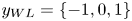 $y_{WL}=\{-1, 0, 1\}$. Inset shows the relative attunement of the centreline temperature with the Widom-line transition temperature,
  $\Delta T_{WL,ctr}\equiv (\tilde {T}_0(0)-\tilde {T}_{WL}(0))/\tilde {T}_{WL}(0)$, for baseflows with different prescribed
  $y_{WL}$. (b) Profiles of isothermal compressibility for three example baseflows with various prescribed locations of Widom-line transition, demonstrating the enhanced sensitivity of the thermodynamic response.
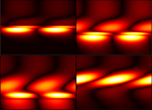
Figure 5 plots the most unstable eigenmode for the axial velocity perturbation  $|\hat {u}|$ and the reconstructed perturbation field at
  $\alpha =0.5$ and
  $P_r=1.18$, for
  $y_{WL}={0, -0.5, -1.0, -3.0}$. Here, the eigenmodes are normalized by their maximum amplitude and the eigenmode for the ideal-gas configuration is also plotted for reference. Note that comparisons between the magnitudes of the eigenmodes in figure 5 should not be performed because eigenmodes have no absolute scale in the LSA framework. Through these visualizations, we note the superposition of two different instability mechanisms near the centreline. One is the classical binary mixing layer instability that arises from the baseflow's inflection point, corresponding to the upper and smoother structure. The other is the thermodynamically induced instability that arises from the sharp variations in thermodynamic response functions, corresponding to the lower and sharper structure. As the Widom-line transition location
  $y_{WL}$ shifts away from the centreline, the classical binary mixing layer instability remains at the inflection point at
  $y=0$. In contrast, the location of the thermodynamically induced instability shifts in accordance with
  $y_{WL}$, see the evolution of the reconstructed axial velocity perturbation as
  $y_{WL}$ is varied in the four panels of figure 5. Concurrently, with detuning of the Widom-line transition location
  $y_{WL}$ away from the centreline, the classical binary mixing layer instability is amplified compared with the thermodynamically induced instability. This is caused by the thermal shielding effect of enhanced heat capacity across the Widom-line transition being lessened at the centreline. In contrast, as
  $y_{WL}$ shifts away from the centreline, the thermodynamically induced instability is attenuated compared with the hydrodynamically induced instability, as there is a reduction in thermodynamic-property gradient required to activate the regions of high sensitivity in the thermodynamic response functions. Eventually, when
  $y_{WL}=-3$, the thermodynamically induced instability vanishes and the perturbation mode recovers towards that of the ideal-gas Kelvin–Helmholtz instability.

Figure 5. Reconstructed axial velocity perturbation  $u_1$ (left side of graphs) and corresponding profiles of axial velocity perturbation mode
  $\mid \hat {u}\mid$ (right side of graphs) at
  $\alpha =0.5$ for cases with
  $P_r=1.18$ and
  $y_{WL}=\{0, -0.5, -1.0, -3.0\}$. (a)
  $y_{WL}=0$. (b)
  $y_{WL}=-0.5$. (c)
  $y_{WL}=-1.0$. (d)
  $y_{WL}=-3.0$.
Overall, the net effect of aligning the Widom-line transition condition with the binary mixing layer's hydrodynamic inflection point is to destabilize the flow by introduction of the thermodynamically induced instability mechanism, see figure 6. Specifically, as  $y_{WL}$ shifts away from zero, variations in the thermodynamic response functions become less prominent at the hydrodynamic inflection point at the centreline. This effect leads to the reduction and eventual vanishing of the thermodynamic-dominant backward-travelling eigenmode as well as the tightening of the instability envelope of the hydrodynamic-dominant forward-travelling eigenmode. Eventually, when
  $y_{WL}$ is sufficiently far away from the inflection point, the effects of the thermodynamic response functions on the binary mixing layer hydrodynamics vanishes and the instability envelope recovers towards that of the ideal-gas binary mixing layer instability.

Figure 6. (a) Destabilizing influence of the alignment between thermodynamic Widom-line transition point and the binary mixing layer hydrodynamics on the temporal growth rate. Solid lines indicate backward-travelling eigenmode and dashedlines forward-travelling eigenmode. (b) Maximum temporal growth rate as a function of wavenumber  $\alpha$ and location of Widom-line transition
  $y_{WL}$. Results are shown for
  $P_r=1.18$.
4. Conclusions
The stability dynamics of binary mixing layers at supercritical pressure conditions was studied using LSA, in which real-fluid effects were considered using the PC-SAFT EOS. Specific focus was placed on examining the effects of strong variations in thermodynamic response functions across the Widom-line transition on the underlying binary mixing flow instability.
Results from the stability analysis show behaviours substantially different from previous studies of single-species mixing flows at supercritical conditions and of classical compressible mixing flows in ideal-gas conditions. Specifically, when the Widom-line transition location is colocated with the binary mixing layer's inflection point, we showed that the binary mixing layer is destabilized by the effects of supercritical real-fluid thermodynamics at the degenerate phase transition condition. Furthermore, it is shown that the destabilizing effect of supercritical real-fluid thermodynamics on binary mixing flows is brought about as a result of strong variations in the thermodynamic response functions at the Widom-line transition, which, when in close proximity with the binary mixing layer's inflection point, can take advantage of the existing flow perturbations to develop into a new instability mechanism that interacts with the existing Kelvin–Helmholtz instability. Thus, the strength of this thermodynamically induced instability is directly correlated to (a) the strength of real-fluid thermodynamic effects across the Widom-line transition, which diminishes with increasing pressure past the critical point and (b) the attunement between the location of Widom-line transition with the inflection point of the underlying binary mixing layer.
The coexistence of the thermodynamically induced and the hydrodynamically induced instability mechanisms uncovered in the present paper for supercritical mixing flows bears striking analogies with the dual-mode instability behaviour of supercritical boundary layers observed by Ren et al. (Reference Ren, Marxen and Pecnik2019b). Thus, the results of the present study highlight the need for fundamental research into the universal coupling between Widom-line dynamics and hydrodynamic instabilities, as well as for an extension of classical instability criteria (e.g. Rayleigh criterion and Fjørtoft's extension) to incorporate the effect of real-fluid thermodynamic response functions.
Finally, the exploitation of this instability mechanism offers opportunities for improving fuel injection systems operating at high pressures, such as diesel and rocket engines (Mayer et al. Reference Mayer, Telaar, Branam, Schneider and Hussong2003; Koukouvinis et al. Reference Koukouvinis, Vidal-Roncero, Rodriguez, Gavaises and Pickett2020). Specifically, while Banuti & Hannemann (Reference Banuti and Hannemann2016) demonstrated that the mixing performance in single-fluids injectors can be improved by the potential core crossing the Widom line axially, we show in this paper that binary mixing flows feature another mechanism for enhanced mixing by crossing the Widom line vertically across the splitter plate.
Funding
This work is supported by Stanford University School of Engineering Fellowship; NASA Space Technology Graduate Research Opportunities, NASA Award no. 80NSSC20K1171; and the US Department of Energy, Basic Energy Science with Award DE-SC0021129.
Declaration of interests
The authors report no conflict of interest.


 Open access