


Introduction
Sea ice is subject to constant changes. Ice drift and deformation are influenced by forces from wind and ocean currents, by obstacles such as islands and coastlines and by ice thickness and roughness variations in a given area. Satellite-borne imaging sensors, operating in the optical and in the microwave range of the electromagnetic spectrum, are used for continuous monitoring of sea-ice-covered regions.
The main advantage of microwave data compared to optical imagery is that they are independent of weather and light conditions. For more detailed studies of sea-ice drift, synthetic aperture radar (SAR) images have been successfully used since the launch of European Remote-sensing Satellite ERS-1 (Reference Holt, Rothrock, Kwok and CarseyHolt and others, 1992). SAR imaging modes with different spatial coverage and resolution make it possible to investigate drift patterns at different scales. Our systematic analysis of different SAR image types indicates that the possibility to select between data acquired at different polarizations may enhance the reliability of the drift and deformation patterns derived from sequences of SAR images.
For the last three decades, various approaches have been applied to extract sea-ice drift information automatically from SAR data. One of the first approaches was described by Reference Hall and RothrockHall and Rothrock (1981). the first operational system was implemented at the Alaska SAR Facility by Reference Kwok, Curlander and PangKwok and others (1990). the range of approaches covers feature tracking, floe tracking, statistical methods and optical flow-based algorithms, as described by Reference Gutierrez, Long and SteinGutierrez and Long (2003).
Some of the employed approaches are based on the tracking of pixel patterns such as that described by Reference Fily and RothrockFily and Rothrock (1987) while others first use a classification step to identify objects for tracking (Reference BanfieldBanfield, 1991; Reference McConnell, Kwok, Curlander, Kober and PangMcConnell and others, 1991). Recent work by Reference Thomas, Geiger and KambhamettuThomas and others (2008) is based on pattern recognition to identify the change of positions of recognizable structures in the ice cover between successive SAR scenes. Hence, it depends on the assumption of temporal pattern stability.
However, sea-ice deformation changes existing patterns and violates the ‘constancy constraint’. It is therefore necessary to acquire data with a sufficiently high temporal resolution which varies depending on the typical drift velocities in the area of interest. the temporal resolution also determines the accuracy of the displacement vector field derived from an image pair. the displacement vector represents the shortest distance between the respective positions of a reference point. the true path of the latter, however, may deviate considerably from a straight line between the two positions (e.g. due to the influence of varying wind directions and/or tidal currents). Any variations of the drift pattern between the two snapshots are unknown.
The first part of the paper deals with the description of the implemented method and the SAR data used for testing the algorithm. the implemented method is one of the most recent pattern-based tracking approaches and shows promising results for high-resolution sea-ice drift estimation from SAR satellite data (Reference Thomas, Geiger and KambhamettuThomas and others, 2008). To estimate the reliability of the method, it is crucial to quantify the magnitude of the error. Another central point of this paper is to establish criteria predicting the performance of the algorithm depending on ice-cover characteristics and image features such as the texture entropy.
In order to increase the spatial coverage, as well as to study details of drift and deformation in key regions, it is necessary to use data of different spatial resolution and swath widths and to quantify the differences in the estimated drift. Here comparisons between Image Mode (IM) and Wide Swath Mode (WS) products from Envisat Advanced SAR (ASAR) are presented. Finally, the results of this work are discussed and an outlook on future work is provided.
Method
The ice-drift algorithm used is based on a concept outlined by Reference ThomasThomas (2008) and Reference Thomas, Geiger and KambhamettuThomas and others (2008). In the original algorithm, global motion (inital motion vector) was estimated in advance either based on buoy data (Reference ThomasThomas, 2008) or based on an assumed phase correlation (Reference Thomas, Geiger and KambhamettuThomas and others, 2008). In our implementation, the initial motion vector is determined in the same way as subsequent vectors on finer scales (see the description of the algorithm below). Subpixel accuracy was not included in the recent version of our implementation. One reason for this was to minimize the computational cost, which is an important aspect if sea-ice drift needs to be determined over a larger area and a longer time period.
Robustness against noise is an important criterion for the choice of a drift retrieval algorithm. To achieve a high robustness, the correlation module is embedded into a cascading resolution pyramid. It is based on a normalized cross correlation (NCC) with a preceding candidate selection. the candidates are selected by employing phase correlation, an approach which is described by, for example, Reference CantyCanty (2007). All correlation peaks higher than 75% of the maximum peak obtained from phase correlation are stored as candidates to be analysed employing the NCC. If the phase correlation does not provide an unambiguous result (>25% accepted correlation peaks), the region is regarded as distorted and an error flag is returned. the NCC has to be carried out in the spatial domain due to the nonlinear terms introduced by the normalization employing the standard deviation (division and squares), which cannot be carried out within a convolution kernel (Reference Gonzalez and WoodsGonzalez and Woods, 2008). the application of two independent correlation measures increases the stability of the algorithm. Additionally, the algorithm runs in a computationally efficient manner since phase correlation can be performed efficiently in the Fourier domain.
The algorithm starts at the coarsest resolution level with a search window covering the full scene. on the second coarsest resolution level, the numbers of rows and columns of the scene double while the number of pixels in the search window stays the same which now covers a quarter of the full scene. For the calculation of position changes at the second level, the result of the first level is used as the initial shift and the resulting four shift vectors of the current resolution level are handed over as the initial shift to the next higher level. the next higher resolution level again contains four times more pixels, and the calculated shift vectors are used to initialize the calculations for the next step until the bottom of the resolution pyramid is reached.
The number of resolution levels and cascade runs are defined by the user. This procedure reduces the sensitivity to noise and increases the robustness of the algorithm, since the initial vectors are based on the resulting vectors of the previous cascade representing the estimated central shift for each search window. Due to this initial information, the algorithm searches in the predicted direction. Since the correlation module returns an error flag if a correlation ‘fails’, data gaps occur which would inhibit shift estimation on subsequent resolution levels. To avoid this and to reduce the influence of outliers on successive calculations, the data are regularized using a running box median filter followed by a triangulation-based interpolation to fill existing data gaps. the interpolation is performed using quintic polynomials (Reference AkimaAkima, 1978).
In order to assess the quality of the results, the calculated values are compared with manually collected reference data. the reference vectors represent the shift of one specific identifiable object or pixel within the enclosing resolution cell, while the algorithm calculates a central shift for the whole cell. the comparison of both shifts is therefore, strictly speaking, only valid for uniform shifts within the respective resolution cell. the manually determined shift is also prone to errors. the appearance of distinct objects in the two images is sometimes slightly different, which makes it more difficult to determine the positions of matching reference points on a pixel scale. One way to estimate the magnitude of reference errors is the collection of two or more independent reference datasets.
When applying the drift retrieval algorithm described above, we assume that both images are precisely geocoded. the comparison between the results of pattern recognition and the manually derived dataset (which is a result of visual pattern recognition) is a quality control for the former since, in both approaches, only the two SAR images are compared. However, for estimating the absolute error of the obtained drift vectors, independent datasets such as drift buoy tracks and/or land-based control points are required. In this case, the geolocation errors of the SAR images and the reference drift patterns also have to be taken into account. For our SAR images we could not find suitable drift buoy data for comparision and the scenes did not cover land.
Methods based on pattern recognition calculate the spatial shift of a resolution cell from one point in time to another. Sea-ice drift refers to a velocity, i.e. a change of position within a certain time period. To compare the performance of the algorithm for different resolutions, the shift (motion) is presented as pixels. Calculated shift data can be converted to velocity by normalizing them to the time difference between the respective image acquisitions.
In practical situations, the retrieval of ice drift patterns is more difficult if the ice cover appears homogeneous in the image, without clearly recognizable structures. Hence, it is useful to check whether a given algorithm can be applied for given sea-ice conditions. For the algorithm used in this study, the correlation coefficients for each single resolution cell were compared to different texture parameters such as entropy and variance.
Data
The Envisat ASAR data used for the analyses presented in this paper were acquired in 2006 in the Weddell Sea close to the grounded A-23A iceberg. the overlaps for each of the selected image pairs cover regions of at least 100 km × 100 km. the data are from the end of January, middle of June and end of August. For all three periods it was possible to order two IM SAR images. For the periods June and August, corresponding WS data could be ordered in addition to the IM data. Level 1b data products were used.
While the June and August datasets show numerous stable patterns, the patterns in the January scene change considerably due to the season (Antarctic summer). Prior to drift calculations, the images were geocoded and calibrated using commercial remote-sensing software. the drift in the IMdata was determined using a five-level resolution pyramid within a six-stage cascade to create 512 × 512 resolution cells. the drift values from the WS data were obtained on the basis of a four-level image resolution pyramid within a five-stage cascade, creating 128 × 128 resolution cells. the amount of extractable cells depends on the extent and spatial resolution of the scene. Experiments show that the size of a resolution cell should not be smaller than ∼10 × 10 pixels in order to extract a stable shift vector field. These values are based on a close examination of the amount of data gaps and resulting resolution. A smaller resolution cell would grant a higher resolution of the drift field but would also contain more data gaps due to the smaller significance of corresponding image patterns.
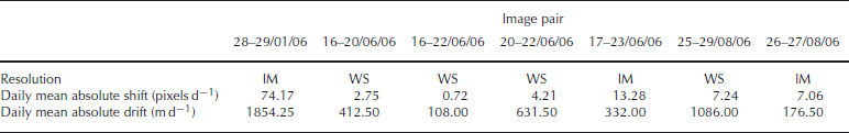
The accuracy of the automated procedure was determined in comparison to manually derived reference datasets as described above. the number of collected vectors per image pair varies between 133 and 151. Details of the SAR scenes, the parameters required for the automated procedure and the reference datasets are summarized in Table 1.
Table 1. Properties of test Envisat ASAR datasets. the original resolution refers to the image product, and the resampled resolution to the post-processed data products used for the drift calculation. the position of the overlap area is indicated by the coordinate of the upper left corner (UL). the drift algorithm calculates a drift for square regions (referred to as resolution cells). the covered area per resolution cell is called shift resolution. Dates are dd/mm/yy

Results
The spatial resolution of the resulting drift vector fields is 300m in the IM data and 1200 m in the WS data. Since we use geocoded images, the x and y axes (image coordinates) correspond to the south–north (SN) and west–east (WE) directions. Mean absolute velocities for the observed cases are 110–1850md − 1. Table 2 shows the mean absolute displacement per day in pixels and metres. the apparently inconsistent results for June can be explained by fast variations of wind direction and speed.
Table 2. Mean absolute displacement of the sea ice for the observed time period, normalized to 1 day (24 hours). the results for June are discussed in the text
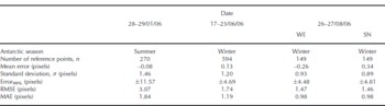
To generate larger datasets for statistical analysis of the errors, the differences between the algorithm and the reference are combined independently of direction where possible. It was therefore checked whether the error is direction-dependent using a two-sample Kolmogorov– Smirnov test. the null hypothesis H 0 states that the WE and SN errors come from the same distribution. the alternative hypothesis H 1 states that they come from different distributions. the IM error distributions for January and June do not depend on the direction at the 95% confidence level. For the August IM dataset, H 0 is rejected at the 95% confidence level. Based on the test results, errors in the WE and SN directions are combined for January and June but examined individually for the August period. Student’s t -distribution is fitted to all four IM error distributions. All error values are within the 95% confidence bounds of the corresponding Student’s t -distribution.
The calculated error statistics for the IM-based shift vector fields are listed in Table 3. For June and August, 99% of the calculated error values are within ±5 pixels, which corresponds to ±125m in the IM images. With a time difference of 5.8 days (IM image pair from June), the error of the drift velocity is 22 md − 1. With 1.19 days (IM image pair from August), it is 105 md − 1. These values have to be related to the estimated daily mean absolute drift shown in Table 2.
Table 3. Error statistics for IM data: dates of data acquisition, number of used reference displacement vectors n, the calculated mean error based on the used reference data (as well as the standard deviation of the error), the error margin representing 99% of the error, the mean absolute error (MAE) and the root mean square error (RMSE)
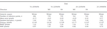
For January (summer conditions), the error is ±12 pixels, corresponding to a displacement error of ±300 m. Error distributions for the August WS drift field and the 16–20 June WS data do not depend on the direction, while the error distributions for the 16–22 June WS and 20–22 June WS do. Since the position shift is estimated in numbers of pixels, the different error measures are also given as a number of pixels. As the errors for June and August are of almost identical magnitude in the SN and WE directions, it is reasonable to assume a lower bound of the spatial shift below which any displacement cannot be resolved reliably.
Reference ThomasThomas (2008) notes that a mean absolute percentage error (MAPE) of 10% is generally used as a reasonable metric in many practical applications. the goal is to give a limit for the estimated shift value below which the relative error has to be considered in subsequent applications. the absolute percentage error is calculated for each reference point individually. It is described as the absolute difference between reference shift and estimated value, divided by the absolute reference shift. In order to estimate the minimum shift fulfilling this criterion, the mean absolute error (MAE) is used (Tables 3 and 4). the lower bound of the magnitude of the shift vector is therefore about ten times the MAE, meaning 8–12 pixels for June and August (200–300m and 1200–1800 m, respectively) and about 18 pixels for January (450 m).
Table 4. Same as Table 3, but for WS data
The relative error of a shift vector depends not only on the existence of constant patterns but also on the velocity of the related drift. In case of a slow drift, a short observation time might result in a positional shift not fulfilling the 10% criterion, while a longer observation time (with pattern constancy) might do. (The related lower bounds for the drift are calculated from the pixel shift bounds, converting them to a distance in metres based on the given resolution information. the limiting velocity is calculated by normalizing this distance to the time difference of the data pair.) the resulting lower bounds for the drift in the selected IM examples are 388md − 1 (0.005ms − 1) for January, 51 md − 1 (0.0006ms − 1) for June and 206md − 1 (0.002ms − 1) for August. the resulting lower bounds for the WS examples are 210–690md − 1 (0.002–0.008ms − 1).
The comparison of two manually generated independent reference datasets of the sea-ice drift for June shows that the error between the reference shift and the central drift of the enclosing resolution cell, as well as of the error introduced by the manually collected reference data, is about ±1 pixel (25m). This observation also makes sense given that there is no subpixel tracking for the reference data collection.
Figure 1 shows the results for the August data. the shape of the image boundaries is determined by the overlapping area between the two successive SAR images used for the derivation of the ice shift. In the figure, the estimated shift (left) is presented together with a gap map showing the positions of resolution cells where the matching algorithm returned an error flag (right). the corresponding pixels are marked by black dots. the overlap area covers the southern part of iceberg A-23A (upper left), surrounded by sea ice. In the western part, open water patches are visible with smaller icebergs. the key feature of the scene is a long lead dividing the ice cover into a western and an eastern part. While the sea ice in the western part of the scene is brought to a halt by iceberg A-23A in the north, it drifts comparatively fast northeastwards in the eastern part of the scene.

Fig. 1. Drift and data gaps of the August IM dataset. Left: data acquired on 26 August 2006 combined with the calculated drift between 26 and 27 August 2006; right: data gaps indicating regions (black dots) for which the algorithm failed to calculate reliable shift information and returned an error flag.
Studying the gap map reveals that the algorithm fails in some regions while it works perfectly well for others. Large icebergs can be easily detected by the increased number of correlation failures. This is also valid for leads and low-contrast regions such as in the southeast in Figure 1. Results for the January and June datasets also support this conclusion.
In order to identify other methods that help to assess the expected performance of the algorithm from the characteristics of the image, the correlation coefficient of each resolution cell was plotted against different texture parameters such as entropy and variance for the respective cell. Entropy is a measure used in information theory describing the uncertainty associated with a value. Minimum values occur for uniform regions while maximum values occur for heterogeneous regions with n equiprobable values for n texture pixels, as first described by Reference ShannonShannon (1948):
where p(xi ) is the probability mass function of outcome xi .
Equation (1) is employed as a measure of local textural heterogeneity. From the investigated parameters, a meaningful relationship was obtained only for the texture entropy (Fig. 2) but not for measures such as uniformity, registrability and intensity. Registrability is a measure developed by Reference ChalermwatChalermwat (1999) for high-performance image registration for remote sensing.
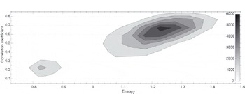
Fig. 2. Relation between entropy and correlation coefficient: a simplified 2-D histogram based on entropy values for each resolution cell and their corresponding median-filtered correlation coefficents. the data density is indicated with a greyscale.
Two separated data clusters can be recognized in the two-dimensional (2-D) histogram (Fig. 2): a smaller group in the lower left corner with an entropy of 0.8–0.9 and a correlation coefficient of 0.1–0.3 and the main group with an entropy of 1.04–1.42 and a corresponding correlation coefficient of 0.35–0.85. the maximum observed entropy is 1.70. To reduce the variation in the data and to emphasize the correspondence between entropy and performance of the algorithm, the histogram is calculated based on preprocessed shift data which were filtered with a 5×5 median filter. the correlation coefficient for this relation is 0.75. While the smaller data cluster is only a significant feature for the August dataset, caused by the huge influence of A23-A on this scene, it is possible to find relations similar to the main group for January and June.
Higher entropy (local heterogeneity) indicates a higher probability of the occurrence of characteristic patterns in the sea-ice structure seen by the radar. In this case, the correlation coefficient between corresponding areas in successive images is higher. A low entropy value for a region indicates a lack of characteristic patterns, which may lead to worse correlation results. A lower entropy is linked with less local variation of the radar intensity. Compared with the sea-ice cover in the August scene, iceberg A23-A appears quite homogeneous. the correlation between entropy and (pattern) correlation coefficient is, however, only moderate. This indicates that the performance of the algorithm depends not only on the entropy but also on other image characteristics such as the presence of distinct patterns.
The result suggests that an entropy greater than 1.00 indicates good correlation conditions but with some restrictions due to the levelling nature of filtered values. Regions of high entropy cannot be correlated if patterns are different in the two images used for shift vector retrieval.
The third topic of this paper is the comparison of motion fields estimated from ASAR IM data with those from WS data. Figure 3 shows the corresponding results. the field of shift vectors calculated from the IM data is less homogeneous than that extracted from the WS mode where the flow field is more uniform. Key features of the drift field remain recognizable at the lower resolution level. To compare the results statistically, the IM shift vector field is smoothed and resampled to the resolution of the WS data. Both datasets are normalized to 1 day, assuming constant drift conditions during the observation period. Subsequently, the difference between the vector fields is calculated separately for the WE and SN components of the drift. the mean absolute distance between the WS shift and resampled IM shift is about 1 pixel (150 m) in the WE direction and 2 pixels (300 m) in the SN direction, with a corresponding RMSE of 2.64 pixels (400 m) in the WE direction and 3.73 pixels (560 m) in the SN direction.

Fig. 3. August drift vector field and August WS drift vector field. Left: results for the IM data pair; right: WS results.
Major differences in the drift field between the two datasets are caused by the different scales. the high-resolution vector field follows the shape of the central lead, while in the WS image larger shifts in the east are transferred into the stagnant sea ice in the west and vice versa. the relation between the IM-based drift field and the WS-based drift field is shown in the scatter plot in Figure 4, which illustrates the complex relation between the two motion fields. In contrast to the IM-based drift information, which identifies smaller motion variations even at the coarser resampled resolution, the WS-based motion field shows a more levelled drift. Both directions resolve the stable sea-ice situation south of iceberg A23-A.

Fig. 4. Scatter plot of IM-based drift versus WS-based speed in WE direction. It shows that in IM images drift field variations are recognized over shorter distances, i.e. in greater detail, than in WS images.
The iceberg itself creates errors due to false correlation results related to its small amount of characteristic patterns. While the IM-based drift data follow the shape of the central lead quite closely, the WS-based motion shows various deviations from the orientation of the lead. East of the lead that divides the scene into two parts, the IM drift vector field shows drift zones of miscellaneous magnitude and direction while the WS data show a more homogeneous drift situation. the IM drift field reveals an eastern shift in the far east of the image, whereas the shift of the WS motion field is a northeastern shift in this region. Additionally, the fact that the image pairs span different time periods must be taken into consideration. Changing conditions during these periods would also lead to changes within the normalized data.
The situation is more complicated for the June period since the extracted drift fields do not show key features common to both imaging modes (IM and WS). the drift field extracted from both WS pairs, 16–20 June 2006 and 16–22 June 2006, fails to reveal drift characteristics similar to the drift field estimated from the IM pair. A direct comparison of shift is therefore not possible. the result of a manual check was that the calculated displacements are correct for all analysed cases. Based on the stable position of the grounded A23-A in all images, the observed change of motion cannot be explained by an erroneous geocoding. Instead it is more probable that a change of motion directions over time occurred, leading to different motion fields for each data pair because of different temporal gaps between the individual images. the change of motion over time is demonstrated on a single feature shown in Figure 5.

Fig. 5. Change of motion over time. Comparison of a characteristic pattern for all data pairs acquired in June 2006. the comparison indicates high variations of drift direction and magnitude. Dates are dd/mm.
Wind data, provided by the Interim Re-analysis (Reference BerrisfordBerrisford and others, 2009) of the European Centre for Medium-range Weather Forecasts, indicate heterogenic wind conditions with large variations in speed and direction for the period 16–23 June 2006. the wind directly affects the sea-ice drift characteristics. Since sea-ice motion is not only driven by the wind but depends also on ocean currents, tides and general sea-ice conditions (e.g. blocking effects by land and between different ice areas), it is difficult to link changes in sea-ice drift directly to changes in wind conditions. the wind data for the August observation period indicate the typical behaviour for the monitored region at this time of the year, with a dominating strong northward wind component.
Conclusion
The multiscale drift retrieval algorithm investigated in this study demonstrates a good performance for the analysed image pairs. A few drawbacks were found in cases for which central assumptions inherent in the algorithm were not valid. the quality of the estimated vector field strongly depends on pattern constancy in the analysed datasets, as the differences between the January dataset (summer) and the June and August datasets (winter) indicate.
In the analysed cases, the absolute error was independent of the magnitude of shift. the relative error therefore depends on the magnitude of shift. If a 10% criterion is used as an acceptable error for the shift, the minimum shift should be higher than 10–12 pixels (250–300 m) in winter (June and August) and about 18 pixels (450 m) in summer (January). Consequently, a longer time period between successive images is needed for slowly drifting ice than for large drift velocities. However, a longer time period increases the risk of violating the pattern constancy constraint.
The method has problems in homogeneous regions such as iceberg surfaces and areas without any features such as ridges and identifiable single floes. Fast-changing ice-cover characteristics such as leads revealed only low correlation coefficients between successive images. It was demonstrated that a relation between entropy and correlation performance exists and that a higher entropy is linked to a better correlation.
A first comparison of WS and IM data revealed that the drift fields estimated from the WS mode compare well with drift data estimated from IM data, although details are lost. In the presented example it was also demonstrated that sea-ice motion may change rather quickly. This is also very important for sea-ice physics since the averaging of heterogenous sea-ice motion fields may cause an underestimation of the ice velocity and the range of direction changes within the observation period, which affects our ability to interpret/reconstruct the observed sea-ice deformation patterns, in particular with regard to minor deformation events.
Our studies will continue with a comparison of motion fields derived from datasets with different spatial resolution, obtained with different imaging modes from different satellites. the goal is to increase the temporal and spatial resolution of the sea-ice motion field for detailed observation of sea-ice deformation.
Acknowledgements
The work of the first author is funded by the Alfred Wegener Institute in the framework of the German Earth Observing Network (Network EOS). We thank J. Hutchings, the scientific editor, and the reviewers for their useful and productive comments which greatly improved the paper.


