


Introduction
It is hard to overstate the importance of a planter to row crop production. The timing of when the planter is used, its size and efficiency, and its utilization of available technology impact yield from the moment the seed is placed in the ground (Nafziger Reference Nafziger1994; De Bruin and Pederson Reference De Bruin and Pedersen2008; Van Roekel and Coulter Reference Van Roekel and Coulter2011). Optimal planter use has a significant impact on farm profitability during planting, which has led to increased producer demand for quality and reliable planting equipment.
Due to mechanization in modern US production agriculture and the scale/size of row crop production, research and development have led to major planter technology advancements over recent years (USDA 2018; Schnitkey Reference Schnitkey2004a; Reference Schnitkey2004b). Like all agricultural equipment, planters have trended toward larger machines with row numbers ranging from 1 to 48 units that can cover 120 feet with a single pass. However, with innovative technology and increased planter size, has come higher sale prices. Considering that machinery expenses make up approximately 40% of total crop expenses, additional scrutiny is being applied to the planter purchasing decision (Ibendahl Reference Ibendahl2015). Agricultural machines have also become highly customizable, giving producers the ability to purchase equipment with features most important for their operations. This also makes buying a planter on the resale market a complex decision, as a planter is not a homogenous machine for all crop farms. Customizable components include frame configuration, drive systems, row units, seed delivery systems, row cleaners, fertilizer and pesticide options, and many others (Wehrspann Reference Wehrspann2010). Overall, this customization has led to highly differentiated products on the used machinery market, causing a large number of planter specific, economic, seasonal, and spatial factors to drive prices.
Popular press articles and private industry research have recently noted shortcomings in available information and data relating to agricultural planter markets (Mowitz Reference Mowitz2018). This has caused market inefficiencies where consumers do not have full knowledge or confidence in what is for sale, thereby hurting sale price due to the associated risk involved. Overall, technological advancements, improved agronomic knowledge, lack of relevant scientific literature, and market complaints are only a few justifications for further economic research relating to agricultural planter resale prices.
The research presented in this work adds to the existing literature by addressing the issues mentioned above. By doing so, these findings can potentially benefit buyers and sellers in the used machinery market directly and impact future economic research with respect to machinery. Fundamental planter components, economic factors, spatial aspects, seasonality factors, type of sale, and other variables were explored to determine their impact on planter values. The overall objectives for this study were to: (1) identify the primary factors that impact planter sale price on the resale market; (2) evaluate the impact of age and condition on planter values; and (3) determine if these factors are similar, or different, across planter makes and sale types.
Data
Data relating to finalized sales were collected from a multitude of auction companies and machinery dealers for sales occurring from 2016 to the middle of 2018. The results were then compiled in Machinery Pete’s “Auction Price Data” database where they were sourced for this research (Machinery Pete 2018). The planter data set initially consisted of 2,818 observations and included information for the final sale price, make, model, manufacturing year, hours of use, condition, sale date, sale type, city and state of sale, and a specs column where auctioneers entered information they deemed relevant. Extensive data cleaning was required, including removing all observations that did not include the manufacturing year and/or make of the machinery, as well as observations listed as “Other” sale type. Characteristics that were listed in the specs column were pulled out manually to create additional factors for comparison across planters.
The data posed some initial challenges related to inconsistencies in the specifications provided where some observations were highly descriptive with information relating to seed systems, meters, drive systems, fold types, monitors, and more. Additionally, there were gaps in the data relating to the total number of row units and/or the spacing on the rows where full information was not included in the sales description. In those cases, necessary data for either row number or row spacing were sourced from online sale catalogs and machinery operator manuals based on make and model of the planter. Other data were provided with no specifications relating to the planter, limiting the number of components studied. This is relevant, as one would hypothesize that the presence or absence of certain features, such as precision plant technology, tracks, etc., could potentially affect the final sale price. Lastly, the lack of variables relating to acres covered, or hours of use, is unfortunate as other studies have found significant results relating to this depreciation factor (Cross and Perry Reference Cross and Perry1995). In this study, the condition ratings of excellent, good, and fair are all that was available to capture use and wear on the machines.
A total of 847 observations were available for analysis, with descriptive observations for sales occurring across 29 states (Figure 1) and the prominent US production areas. Descriptive statistics for the pooled data are presented in Table 1. Group means based on individual makes and row units are summarized in Tables 2 and 3. The models included variables relating to the manufacturer, age, condition, planter structure, sale type, seasonality, and macroeconomic factors to best estimate the primary objective of identifying factors that influence planter resale price.
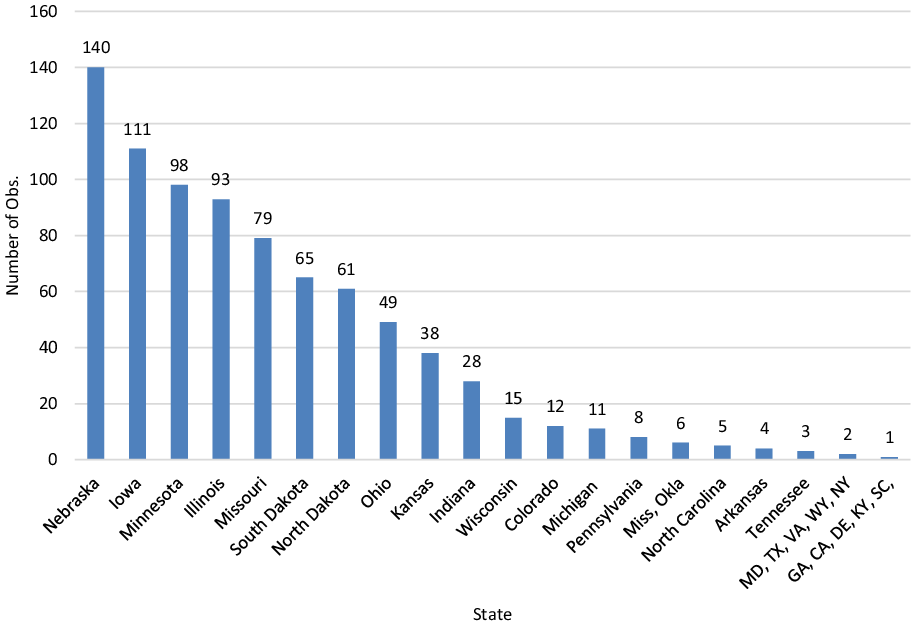
Figure 1. Planter data distribution by state.
Table 1. Planter data distribution and summary statistics
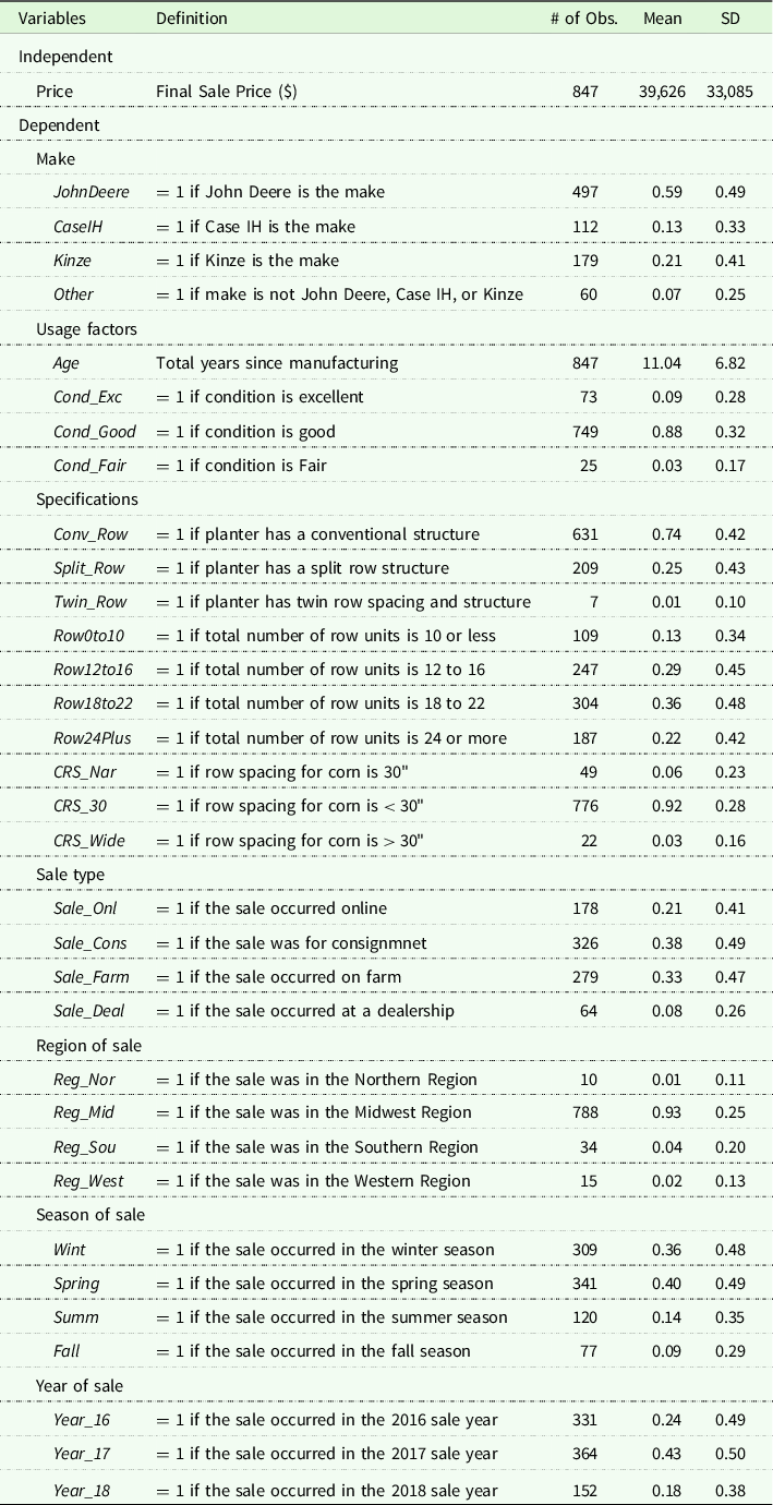
Table 2. Group means for varying makes
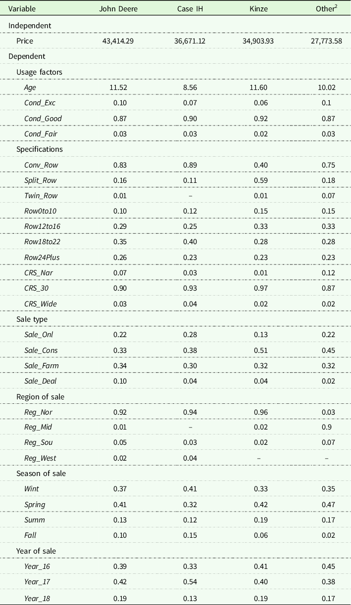
Table 3. Group means for row number groupings

Based on economic and agronomic principles and market trends, expectations were made about the relationship between the explanatory variables and sale price in the base model. When compared to the variable Other makes (grouping of White, Great Plains, Monosem, Peaque, IHC, and Wil-Rich), coefficients for John Deere, Case IH, and Kinze were expected to be highly significant with positive coefficients as seen with previous research related to tractors. Age and age 2 were both expected to impact values and have negative coefficients as seen in prior literature (Diekmann, Roe, and Batte Reference Diekmann, Roe and Batte2008). Naturally, planters in better condition should sell for higher prices, so positive coefficients were anticipated for planters in excellent and good condition, as compared to those in fair condition. Planters with a split row structure are likely to sell at higher price levels due to the increased number of planter components, structural complexity, and increased demand from crop producers in recent years (Mowitz Reference Mowitz2017). Conversely, planters with a twin row structure are likely to see lower prices as they are not highly demanded and their use is almost primarily in the Southern United States.
Row spacing and row number both speak to the planter’s size and were expected to have an impact on sale price. Planters with row spacing at 30” were expected to bring higher prices as that is a common row spacing for corn today and discounts are likely for lower row spacings. The variable for row spacing > 30” is expected to be negative due to these spacing’s no longer being a common practice where yield is not maximized (Lambert and Lowenberg-Deboer Reference Lambert and Lowenberg-DeBoer2003). Larger planters with greater numbers of rows are also expected to sell for higher prices, holding everything else constant.
Having information about sale type has the potential to provide additional perspectives on planter values. Dealer sales were hypothesized to have lower sale values compared to other sale types. This was primarily anticipated because of the competitive nature of the other auction platforms. Location information also allowed for estimation of spatial factors and prices were expected to be higher in the Midwest, which is the predominant growing area for corn and soybeans. Spring was expected to have lower planter values than the other three seasons due to spring planting workload and historical trends (Mowitz Reference Mowitz2018). Year of sale was included in the analysis and can be utilized to capture macroeconomic and profitability factors at that time.
Methods
A hedonic theoretical framework was employed utilizing the data described previously to investigate the factors that drive the value of used row crop planters. The hedonic price method, which was initially introduced by Griliches (Reference Griliches1961) and further developed by Rosen (Reference Rosen1974), has become a popular approach and has been widely employed in modeling the determinants of agricultural land values (Pates et al. Reference Pates, Kim, Mark and Ritter2020; Delbecq, Kuethe, and Borchers Reference Delbecq, Kuethe and Borchers2014; Dillard et al. Reference Dillard, Kuethe, Dobbins, Boehlje and Florax2013; Zhang and Nickerson Reference Zhang and Nickerson2015), commodities (Ethridge and Davis Reference Ethridge and Davis1982), hay (Peake et al. Reference Peake, Burdine, Mark and Goff2019; McCullock et al. Reference McCullock, Davidson and Robb2014), and cattle (Martinez et al. Reference Martinez, Boyer and Burdine2021; Parish et al. Reference Parish, Williams, Coatney, Best and Stewart2018; Burdine et al. Reference Burdine, Maynard, Halich and Lehmkuhler2014). Even before the development of hedonic analysis, factors affecting machinery prices were explored under different theoretical and empirical models. Factors such as horsepower and engine type were used to develop price indices explaining 88–96% of the variation in tractor price in 1963 (Fettig Reference Fettig1963). Duality theory was employed to establish that input/output price ratios and interest rates impacted machinery values (Leblanc and Hrubovcak Reference LeBlanc and Hrubovcak1985).
Previous literature has also revealed the need to continue hedonic research relating to agricultural machinery to ensure accuracy in utilized indices. These factors, paired with the complaints in the industry about inconsistent data collection and consumer knowledge, continue to support research relating to machinery markets (Mowitz Reference Mowitz2018). Hours of use, age, make, sale timing, location, and sale method have been found to impact tractor values in previous work (Diekman, Roe, and Batte Reference Diekmann, Roe and Batte2008). Outside factors such as net farm income and interest rates have also been shown to affect machinery expenditures (Osbourne and Saghaian Reference Osbourne and Saghaian2013) and Wang et al. (Reference Wang, Schimmelpfennig and Ball2013) established the importance of quality on values. However, specific factors relating to agricultural planting equipment prices have not been analyzed in detail. Therefore, the extent of physical machinery components and the extent of outside factors such as commodity prices or sale location have not been explored in relation to planter prices, which lends itself well to the hedonic approach employed in this paper.
The empirical hedonic price model used herein is specified as a linear combination of planter attributes and location characteristics that were defined previously. Under the hedonic price model, planter price is a differentiated product with a bundle of technologies, size and location characteristics, and implicit prices can be estimated based on each characteristic. The planter-specific characteristics include age and row setup. Various sale characteristics such as online, consignment, and auction were considered. Additional variables for region, season, and year of sale are also considered in the model. Equation 1 shows the hedonic regression model implemented:
 $$\ln \left( {{V_i}} \right) = {\beta _0} + {\beta _L}{{\bf{L}}_i} + \;{\beta _W}{{\bf{W}}_i} + {\beta _A}{{\bf{A}}_i} + {\beta _U}{{\bf{U}}_i} + {\beta _M}{{\bf{M}}_i} + {\varepsilon _i}$$
The hedonic regression is formed with the log-linear specification. Because there is no clear theoretical guideline for the correct functional form for hedonic pricing models, a semi-log is preferred as a more flexible form with unobserved attributes or presence of measurement error (Borchers et al. Reference Borchers, Ifft and Kuethe2014). This is a common transformation and has the added benefit of reducing heteroscedasticity. The estimated regression estimated is defined as:
 \begin{align*}\ln \left( {planterpric{e_i}} \right) =& {\mkern 1mu} {\beta _0} + {\beta _1}JohnDeer{e_i} + {\beta _2}CaseI{H_i} + {\beta _3}Kinze_i^.{\rm{ }} \\
& + {\beta _4}Age_i^. + {\beta _5}Age_i^2 + {\beta _6}Cond\_Ex{c_i} + {\beta _7}Cond\_Goo{d_i}{\rm{ }} \\
& + {\beta _8}Spli{t_{Ro{w_i}}} + {\beta _9}Twi{n_{Ro{w_i}}} \\
& + {\beta _{11}}Row18\;to\;{22_i} + {\beta _{12}}Row24Plu{s_i} + {\beta _{13}}CR{S_{{{30}_i}}} + {\beta _{14}}CR{S_{Wid{e_i}}} \\
& + {\beta _{15}}Sal{e_{On{l_i}}} + {\beta _{16}}Sal{e_{Con{s_i}}} + {\beta _{17}}Sal{e_{Far{m_i}}} + {\beta _{18}}Re{g_{Mid}}{\rm{ }} \\
& + {\beta _{19}}Re{g_{So{u_i}}} + {\beta _{20}}Re{g_{Wes{t_i}}} + {\beta _{21}}Win{t_i} + {\rm{ }}{\beta _{22}}Sum{m_i} + {\beta _{23}}Fal{l_i}{\rm{ }} \\
& + {\beta _{24}}Year\_{17_i} + {\beta _{25}}Year\_{18_i} + {\varepsilon _i}\end{align*}
\begin{align*}\ln \left( {planterpric{e_i}} \right) =& {\mkern 1mu} {\beta _0} + {\beta _1}JohnDeer{e_i} + {\beta _2}CaseI{H_i} + {\beta _3}Kinze_i^.{\rm{ }} \\
& + {\beta _4}Age_i^. + {\beta _5}Age_i^2 + {\beta _6}Cond\_Ex{c_i} + {\beta _7}Cond\_Goo{d_i}{\rm{ }} \\
& + {\beta _8}Spli{t_{Ro{w_i}}} + {\beta _9}Twi{n_{Ro{w_i}}} \\
& + {\beta _{11}}Row18\;to\;{22_i} + {\beta _{12}}Row24Plu{s_i} + {\beta _{13}}CR{S_{{{30}_i}}} + {\beta _{14}}CR{S_{Wid{e_i}}} \\
& + {\beta _{15}}Sal{e_{On{l_i}}} + {\beta _{16}}Sal{e_{Con{s_i}}} + {\beta _{17}}Sal{e_{Far{m_i}}} + {\beta _{18}}Re{g_{Mid}}{\rm{ }} \\
& + {\beta _{19}}Re{g_{So{u_i}}} + {\beta _{20}}Re{g_{Wes{t_i}}} + {\beta _{21}}Win{t_i} + {\rm{ }}{\beta _{22}}Sum{m_i} + {\beta _{23}}Fal{l_i}{\rm{ }} \\
& + {\beta _{24}}Year\_{17_i} + {\beta _{25}}Year\_{18_i} + {\varepsilon _i}\end{align*}
The dependent variable in this study is the planter sale price. The variable Age was transformed under the hypothesis that a quadratic relationship between Age and final sale price might exist. Additionally, row number was broken into four groupings (Table 3) to test for a nonlinear relationship between the row number explanatory variable and sale price. These groupings were determined by plotting the residuals pertaining to the variable row number. The pattern of the residuals suggested natural breaks at the row numbers 12, 16, and 24 with linearity between the breaks. Finally, the model was run using Huber/White robust standard errors to handle heteroskedastic issues that were found in the data set.
To explore the potential interaction between the variables, make and Age, the base model was slightly modified. First, an interaction model was estimated using all 847 observations. The interaction model largely included the same variables as the base model, but the Age and Age 2 variables were interacted with the various makes. For the models applied to individual makes, dummy variables representing makes were dropped and no interactions were included; the model was ran separately for John Deere (497), Case IH (112), and Kinze (179).
Results and discussion
Hedonic modeling and STATA software were employed to analyze final agricultural planter sale prices on the used machinery market (StataCorp 2017). In Figure 2, a box and whisker plot was used to demonstrate the distribution of sale prices for all observations as well as for the three primary machinery makes. The mean price across all sale observations was $39,626.19, which was less than the mean value for the market leader John Deere ($43,413.29), but larger than the means for all other makes. Figure 2 provides a simple visual representation of the impact of make on resale price, and regression estimates were found to tell a similar story.
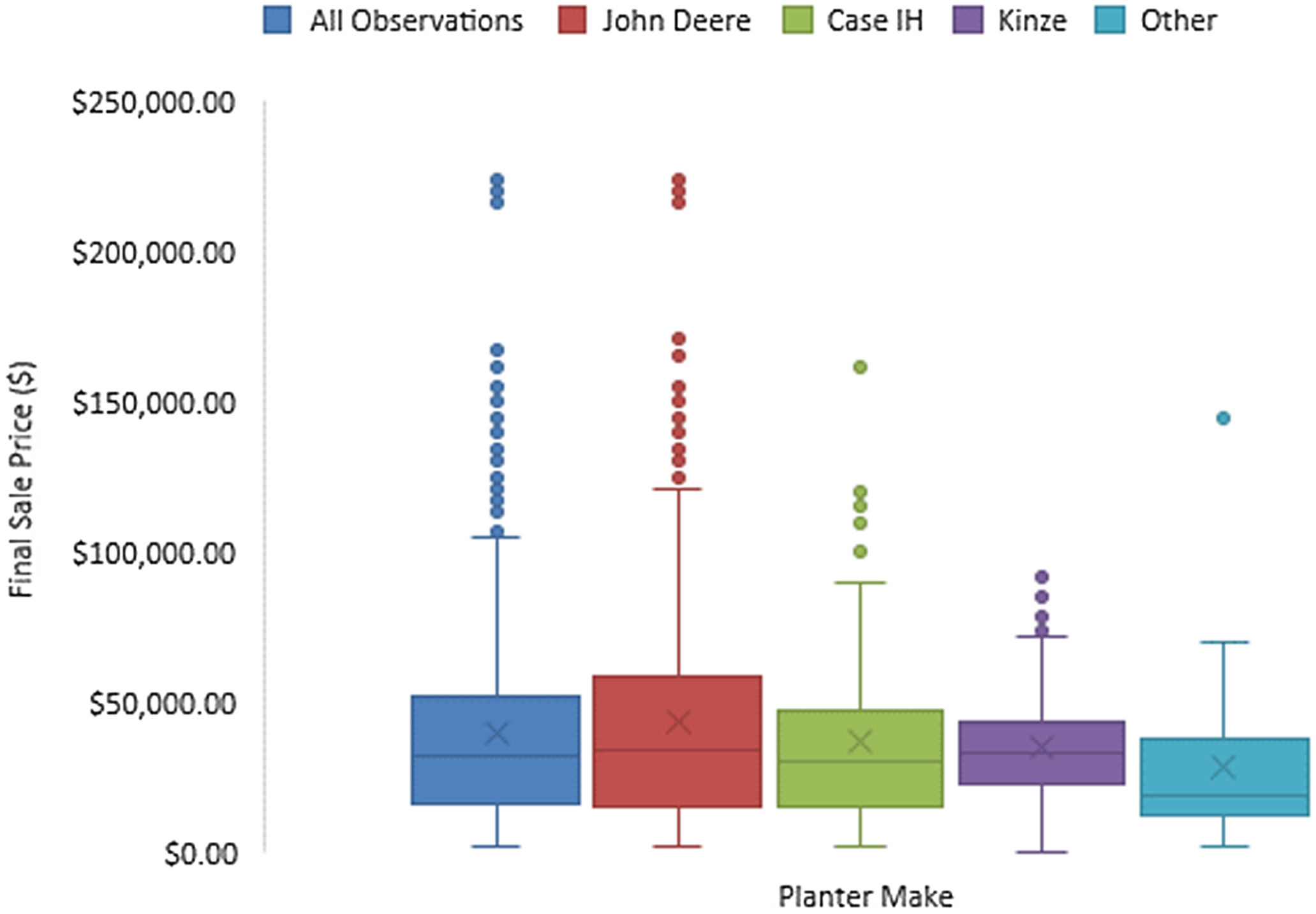
Figure 2. Planter final sale price by make.
The results and estimated coefficients for the base hedonic model are displayed in Table 4. Overall, the model was a good fit for the cross-sectional data with an R 2 exceeding 80%. The model was tested for potential multicollinearity (variance of inflation factor) and specification error (link test), but results did not suggest reason for concern. John Deer, CaseIH, and Kinze had higher sale values than other manufacturers at the 90% level, with John Deere and Kinze having larger impact magnitudes. Not surprisingly, planters in excellent and good condition saw higher prices. And, Age and Age 2 were significant and suggested planters depreciated at a decreasing rate. Split row configuration, all row number groupings, 30” row spacing, >30” row spacing, winter season, and the 2018 sale year were also significant in explaining planter prices. Results also support a stepwise relationship between price and row numbers. It was determined that the impact of row number on price was relative to the size grouping through individual t-tests (t = −2.44, p = 0.008; t = 2.893, p = 0.002; t = 5.37, p = < 0.001). These results also suggest that the marginal impact of an additional row unit is higher for larger planters. This could be influenced by planters being more technologically advanced at a larger size, paired with the decision by producers to upsize, creating more demand for larger planters.
Table 4. Hedonic regression results for base model

*, **, and *** indicate statistical significance at the 90%, 95%, and 99% levels.
A majority of the expected relationships between the variables were confirmed, with the exception of those pertaining to row spacing. Results suggest that when compared to planters with row spacings <30”, 30” and >30” row spacings have a negative effect on a planter’s value. This is potentially driven by the fact that when row spacings are narrower, there is more steel and technology in a given area than a planter at the same width with 30” or >30” rows. Another potential explanation is recent agronomic research showing potential yield benefits from narrow row spacings compared to 30” which is increasing producer demand for these types of planters (Lambert and Lowenberg-Deboer Reference Lambert and Lowenberg-DeBoer2003).
The results for the interaction model can be seen in Table 5 where the fit and significant variables were comparable to the base model results. The inclusion of the interaction terms relating to make and Age is supported by the results where all four interaction variables (JDAge, CIHAge, KinAge, and OthAge) were highly significant at the 1% level. It was further determined through t-tests that JDAge, CIHAge, and KinAge are all significantly different from one another (t = 17.14, p < 0.001; t = 11.15, p < 0.001; t = 5.52, p < 0.001). This could not be said for these three interactions in relation to OthAge which could be a result of data limitations from a small sample size. Overall, these results suggest varying depreciation exists among planters of different makes, and these findings are consistent with previous research relating to other types of agricultural machinery (Perry and Nixon Reference Perry and Nixon1991; Cross and Perry Reference Cross and Perry1995). More specifically, results shown in Figure 3 suggest that Case IH planter values are most negatively impacted by Age when compared to John Deere and Kinze. Somewhat surprisingly, Kinzes retained their value better over time compared to John Deere, which could potentially be a factor of John Deere planters having higher values at the time of manufacturing. This could also be a result of the technology employed on the planters where it could be argued that Kinze’s may be “simpler” than John Deere’s historically. This could also be compounded by a potential niche market existing for these older or “simpler” Kinze planters.
Table 5. Hedonic regression results for base model with interaction terms
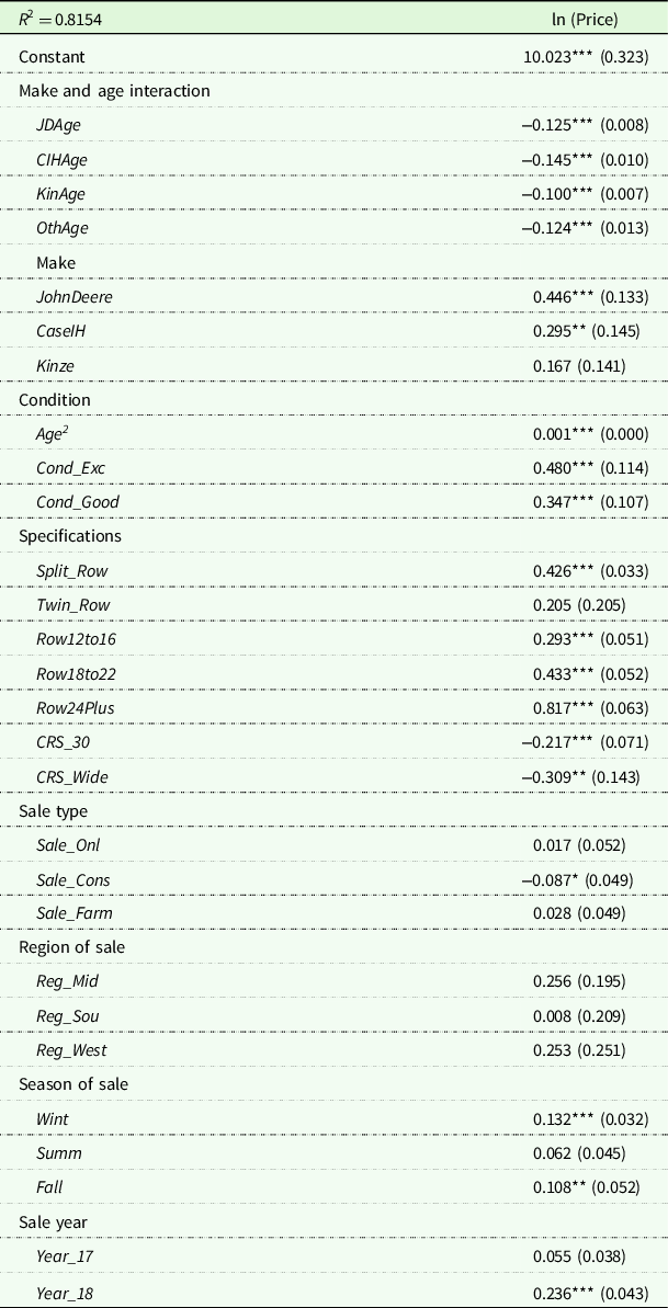
*, **, and *** indicate statistical significance at the 90%, 95%, and 99% levels.
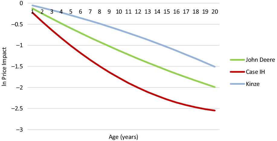
Figure 3. Interaction and quadratic relationship between make and age.
When the model was run for the individual makes John Deere, Case IH, and Kinze, it proved to be a good fit for the subsamples as well (Table 6) with R 2 ranging from 0.81 to 0.85. The highest R2 value was found for John Deere. If this is representative of the true ratio of John Deere planters on the market compared to other makes, it could also suggest that buyers have comparable knowledge of the machine’s perceived value, limiting the unexplained portion of the price variation. Regardless, explanatory power was quite high for all three makes.
Table 6. Hedonic regression results for individual manufacturers
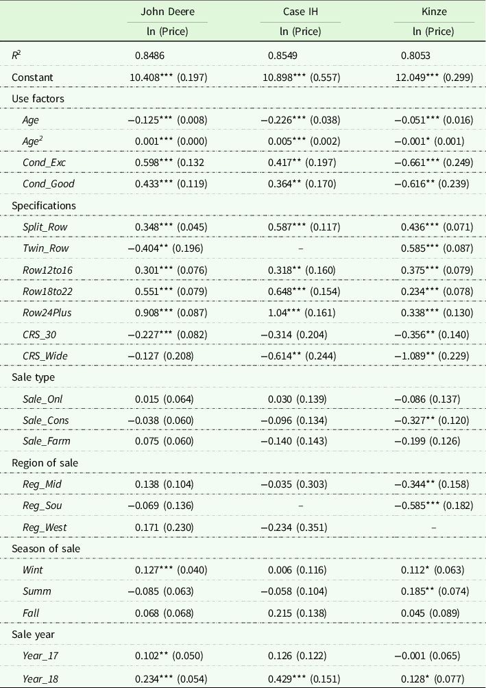
*, **, and *** indicate statistical significance at the 90%, 95%, and 99% levels.
Similar variables were significant across the three makes which included those relating to Age, condition, planter configuration, specifications, and the 2018 sale year. Signs were generally consistent across makes with a few notable exceptions. Interestingly, the twin row variable was significant for both John Deere and Kinze, but their coefficients were opposite. This could be related to areas of focus in research and development by the manufacturers relative to the markets they are potentially targeting. Another interesting and important finding from the individual regressions for different makes relates to the Age and Age 2 variables where the results potentially suggest that there is variable depreciation based on the make. These findings are also consistent with results determined by the interaction model where the impact of age on sale price is dependent on the make of the planter. Age was significant at the 1% level for all three makes, and Age 2 was significant at the 1% level for John Deere and Case IH and at the 10% level for Kinze. Their coefficients suggest a quadratic relationship where John Deere and Case IH lost value at a decreasing rate while surprisingly, Kinze lost value at an increasing rate. Another potential explanation for this variable depreciation relates to demand and brand loyalty, where a recent survey revealed that of the producers surveyed 75% confirmed that they are brand loyal (Kanicki Reference Kanicki2017). Therefore, demand could be higher for certain brands, which assist in the retention of the machines value over time. It was also interesting that Kinze was the only make that was sensitive to sale type and the region of sale.
Conclusions and implications
This work employed hedonic modeling to explore factors that impact planter values on the used machinery market. Results suggest that the primary factors that impact planter resale prices are make, Age, condition, planter configuration, row number, and row spacing. Other factors that showed a significant impact in some cases relate to seasonality and sale year. Surprisingly, sale types and sale location were not found to have a significant impact that was consistent across the varying models in this study.
The other main findings of this research relate to interactive effects between variables and planter values. The variables price and Age were found to have a quadratic relation for planters where in most cases, the price decreases at a decreasing rate as planters get older. Natural breaks were found relating to the row number at 12, 16, and 24, where graphically, the relationship takes on a stepwise shape. Finally, through a model with a focus on interaction terms, it was determined that there is significant interaction between the variables make and Age. The impact of Age on sale price was found to depend on the make of the planter, and for John Deere, Case IH, and Kinze their impact was statistically different from one another. In conclusion, the research conducted here offers highly encouraging results that add to the existing literature and can serve as a base for future research related to agriculture machinery prices on the used machinery market for agricultural machinery.
Acknowledgements
The authors would like to thank Machinery Pete for sharing this data and reviewers for their thoughtful input and suggestions.
Author contributions
JA, TM, KB, and JS conceived and designed the analysis. JA entered and cleaned data, conducted analysis, and wrote initial paper.
Funding statement
This research received no specific grant from any funding agency, commercial, or not-for-profit sectors.
Competing interests
John Allison is employed by Wright Implement but was working on this paper as part of his thesis before accepting that position. Burdine, Mark, and Shockley declare none.


 Open access