


1. Introduction
Collsionless shocks are one of the most ubiquitous phenomena in space plasmas. Collisionless shocks have been in the focus of research for more than half a century, largely because of their efficiency in charged particle acceleration (Axford, Leer & Skadron Reference Axford, Leer and Skadron1977; Bell Reference Bell1978; Achterberg & Norman Reference Achterberg and Norman1980; Toptyghin Reference Toptyghin1980; Lee & Fisk Reference Lee and Fisk1982; Blandford & Eichler Reference Blandford and Eichler1987; Zank et al. Reference Zank, Pauls, Cairns and Webb1996; Giacalone Reference Giacalone2003; Jokipii, Giacalone & Kóta Reference Jokipii, Giacalone and Kóta2007; Zank, Li & Verkhoglyadova Reference Zank, Li and Verkhoglyadova2007). A collisionless shock is a multi-scale phenomenon: the main deceleration and primary thermalization of the bulk plasma flow, as well as ion reflection, occur on a scale of the upstream convective gyroradius or smaller (Hudson Reference Hudson1965; Sckopke et al. Reference Sckopke, Paschmann, Bame, Gosling and Russell1983; Mellott & Greenstadt Reference Mellott and Greenstadt1984; Thomsen et al. Reference Thomsen, Gosling, Bame and Mellott1985; Burgess, Wilkinson & Schwartz Reference Burgess, Wilkinson and Schwartz1989; Sckopke et al. Reference Sckopke, Paschmann, Brinca, Carlson and Luehr1990; Bale et al. Reference Bale, Bale, Mozer, Mozer, Horbury and Horbury2003). The ion distributions at these scales are significantly non-gyrotropic (Sckopke et al. Reference Sckopke, Paschmann, Bame, Gosling and Russell1983, Reference Sckopke, Paschmann, Brinca, Carlson and Luehr1990; Gedalin & Zilbersher Reference Gedalin and Zilbersher1995; Li et al. Reference Li, Lewis, LaBelle, Phan and Treumann1995; Gedalin Reference Gedalin1996; Gedalin, Friedman & Balikhin Reference Gedalin, Friedman and Balikhin2015b; Gedalin et al. Reference Gedalin, Zhou, Russell, Drozdov and Liu2018). Gyrotropization occurs at larger scales due to kinematic gyrophase mixing and wave–particle interaction (Burgess et al. Reference Burgess, Wilkinson and Schwartz1989; Lembège et al. Reference Lembège, Giacalone, Scholer, Hada, Hoshino, Krasnoselskikh, Kucharek, Savoini and Terasawa2004; Bale et al. Reference Bale, Balikhin, Horbury, Krasnoselskikh, Kucharek, Möbius, Walker, Balogh, Burgess and Lembège2005; Krasnoselskikh et al. Reference Krasnoselskikh, Balikhin, Walker, Schwartz, Sundkvist, Lobzin, Gedalin, Bale, Mozer and Soucek2013; Gedalin Reference Gedalin2015; Gedalin et al. Reference Gedalin, Friedman and Balikhin2015b; Gedalin Reference Gedalin2019a,Reference Gedalinb). At the end of the gyrotropization process, ion distributions remain anisotropic. Isotropization is even a slower process and depends strongly on the ion energy. High-energy ion distributions may remain anisotropic far from the shock transition (Kirk Reference Kirk1988; Kirk & Heavens Reference Kirk and Heavens1989; Kirk & Dendy Reference Kirk and Dendy2001; Keshet Reference Keshet2006; Dröge et al. Reference Dröge, Kartavykh, Klecker and Kovaltsov2010; Keshet, Arad & Lyubarski Reference Keshet, Arad and Lyubarski2020). One of the central problems of the shock physics is finding the relation of the upstream and downstream ion distributions. This issue is crucial for establishing Rankine–Hugoniot (RH) relations connecting the upstream and downstream states. the RH relations are nothing but the density, momentum and energy conservation laws, applied in two asymptotically uniform regions. Usually, the RH relations are used on the magnetohydrodynamic (MHD) scales where the distributions are assumed to be isotropic and some equation of state for plasma is chosen (de Hoffmann & Teller Reference de Hoffmann and Teller1950; Sanderson Reference Sanderson1976; Kennel Reference Kennel1988). In most cases the heliospheric shocks do not arrive at the state which can be described by MHD. Near shock transitions, the conservations laws should take into account the non-gyrotropic distributions and corresponding coherent oscillations of the magnetic field. Farther from the shock and with some spatial and/or temporal averaging, the distributions become gyrotropic but anisotropic. Modifications for anisotropic plasmas have also been proposed (Abraham-Shrauner Reference Abraham-Shrauner1967; Chao & Goldstein Reference Chao and Goldstein1972; Lyu & Kan Reference Lyu and Kan1986). Some of modifications invoke assumptions about the state equations. If the anisotropic distributions were known, it would be possible to get rid of arbitrary assumptions. Ion dynamics inside the shock transition is essentially gyrophase dependent. The equations of motion are not integrable even if the electric and magnetic field are time independent, and depend only on the single coordinate $x$ along the shock normal. In a strictly planar stationary shock, the fluxes of mass, momentum and energy must be constant throughout, whereas the momentum vector of an ion at each point behind the shock transition is unambiguously determined by the momentum of the ion at the entry point. This behaviour is expected at rather low Mach numbers $M\lesssim 2\text {--}3$
 . Here the Alfvénic Mach number is $M=V_u/V_A$
 , $V_u$
 being the shock speed relative to the plasma or, in other words, the component of the plasma flow velocity along the shock normal in the shock frame. The speed $V_A=B_u/\sqrt {4{\rm \pi} n_um_i}$
 is the Alfvén speed, $B$
 is the magnetic field magnitude, $n$
 is the number density, $m_i$
 is the ion mass and the index $u$
 denotes the upstream quantities. In this case the density, momentum and energy fluxes are constant throughout the shock which allows one to construct the RH relations for non-magnetized ions as well (Gedalin & Balikhin Reference Gedalin and Balikhin2008). For stationary and planar shocks, the de Hoffman–Teller (HT) frame is well-defined. In the HT frame, the upstream and downstream plasma flow velocities are along the uniform upstream and downstream magnetic field vectors, respectively, whereas the motional electric field is absent. Let $\boldsymbol {p}=(p_\parallel,p_\perp,\varphi )=(p,\mu,\varphi )$
 be ion momentum. Here the subscripts $\parallel$
 and $\perp$
 are used to identify the vector components parallel and perpendicular to the local magnetic field direction, $\varphi$
 is the gyrophase and $\mu$
 is the pitch-angle cosine, $p_\parallel =p\cos \mu$
 . For stationary planar shocks, $\boldsymbol {p}$
 at any $x$
 is determined by the initial momentum $\boldsymbol {p}_i$
 . Individual ion motion in the shock front depends on the initial ion velocity. The properties of the downstream distributions depend on the initial thermal spread which is conveniently characterized by the ratio $v_T/V_u$
 , where $v_T=\sqrt {T/m}$
 is the ion upstream thermal speed. This parameter is related to the often-defined sonic Mach number $M_s=V_u/v_s$
 (Edmiston & Kennel Reference Edmiston and Kennel1984) as $v_T/Mv_A=1/M_s\sqrt {\varGamma }$
 , where $v_s=\sqrt {\varGamma }v_T$
 is the sound speed and $\varGamma$
 is the adiabatic index. Lower $v_T/V_u$
 , that is, higher $M_s$
 , correspond to fewer particles in the tail of the distribution function and, therefore, lower probability of reflection in any part of the shock (Gedalin Reference Gedalin2016). Higher-Mach-number shocks are believed to be time dependent (Lobzin et al. Reference Lobzin, Krasnoselskikh, Bosqued, Pinçon, Schwartz and Dunlop2007; Lefebvre et al. Reference Lefebvre, Seki, Schwartz, Mazelle and Lucek2009; Mazelle et al. Reference Mazelle, Lembège, Morgenthaler, Meziane, Horbury, Génot, Lucek, Dandouras, Maksimovic, Issautier, Maksimovic, Issautier, Meyer‐Vernet, Moncuquet and Pantellini2010; Dimmock et al. Reference Dimmock, Russell, Sagdeev, Krasnoselskikh, Walker, Carr, Dandouras, Escoubet, Ganushkina and Gedalin2019; Turner et al. Reference Turner, Wilson, Goodrich, Madanian, Schwartz, Liu, Johlander, Caprioli, Cohen and Gershman2021) and/or non-planar (Lowe & Burgess Reference Lowe and Burgess2003; Moullard et al. Reference Moullard, Burgess, Horbury and Lucek2006; Lobzin et al. Reference Lobzin, Krasnoselskikh, Musatenko and Dudok de Wit2008; Johlander et al. Reference Johlander, Schwartz, Vaivads, Khotyaintsev, Gingell, Peng, Markidis, Lindqvist, Ergun and Marklund2016). In this case the fluxes are only approximately constant throughout the shock. Upon appropriate spatial and temporal averaging the gyrophase information is lost and magnetic oscillations are smoothed out. Gyrotropic RH relations correspond to the equality of the upstream and downstream fluxes after gyrophase averaging (Gedalin Reference Gedalin2017). In oscillating, rippled or reforming shocks, or when waves are propagating across the shock, there is no one-to-one correspondence of the upstream momentum of an ion and its momentum at each coordinate $x$
 in the downstream region. When the gyrophase information is lost or averaged out, an ion with the reduced initial momentum $(p_{i,\parallel },p_{i,\perp })$
 will not have a definite $(p_{f,\parallel },p_{f,\perp })$
 at a chosen point $x$
 but there will exist some probability of the ion having $(p_{f,\parallel },p_{f,\perp })$
 at the point $x$
 . Such probabilistic approach can be applied for arbitrarily turbulent shock transitions. Instead of trying to solve the deterministic equations of motion, we can describe ion motion as probabilistic scattering at the shock front. Unfortunately, an analytical calculation of the scattering probability is not possible in general case, and numerical methods are to be used. This approach has been successfully implemented already for high-energy particles at a shock front (Gedalin, Dröge & Kartavykh Reference Gedalin, Dröge and Kartavykh2015a, Reference Gedalin, Dröge and Kartavykh2016a,Reference Gedalin, Dröge and Kartavykhb). In the present paper, we develop a theoretical background for the application of such probabilistic approach for the calculation of the moments of the distribution function and derive the probabilities for directly transmitted ions (Gedalin Reference Gedalin2016; Zhou et al. Reference Zhou, Gedalin, Russell, Angelopoulos and Drozdov2020; Gedalin Reference Gedalin2021) in the narrow shock approximation.
2. Basic definitions
The underlying assumption is that far enough from the shock transition, in the upstream and downstream regions, the magnetic fields and plasmas are uniform and the distributions are gyrotropic but not necessarily isotropic. The analysis will be done in HT frame where the motional electric field is absent in both uniform regions. If a shock is stationary and planar, there exists an electrostatic field $E_x(x)$ inside the transition region, so that the cross-shock potential is

where $x$ is the coordinate along the shock normal and $E_x=0$
 for $x<0$
 . Other coordinates are chosen so that $B_y=0$
 in both uniform regions. Hereinafter, the subscripts $u$
 and $d$
 denote upstream and downstream, respectively. The uniform magnetic field and velocity vectors are


Here ${\rm sign}(x)=1$ for $x>0$
 and ${\rm sign}(x)=-1$
 for $x<0$
 , whereas $\hat {x}$
 and $\hat {z}$
 are unit vectors in $x$
 and $z$
 directions, respectively. The sign of the plasma velocity is chosen so that the positive direction of $x$
 is from upstream to downstream. We also refer to the normal incidence frame (NIF), in which the upstream plasma velocity is along the shock normal. For brevity of expressions, in what follows, we restrict ourselves with non-relativistic velocities, including the relative velocity of the frames $\boldsymbol {V}_{NIF\rightarrow HT}=(0,0,V_u\tan \theta _u)$
 , so that for each particle $\boldsymbol {v}_{HT}=\boldsymbol {v}_{NIF}+\boldsymbol {V}_{NIF\rightarrow HT}$
 :
:


and $v_\perp ^2=v^2-v_\parallel ^2$ . However, some relations will be given in a fully relativistic form for future use. In the chosen non-relativistic limit, the magnetic fields are the same in both frames, whereas the electric fields are related by the expression: $\boldsymbol {E}_{NIF}=\boldsymbol {E}_{HT}+\boldsymbol {V}_{NIF\rightarrow HT}\times \boldsymbol {B}/c$
 . The last expression means that there exists the motional electric field $E_{y,NIF}=V_uB_u\sin \theta _u/c$
 and that the cross-shock electrostatic fields and potentials are different in both frames (Formisano Reference Formisano1982; Goodrich & Scudder Reference Goodrich and Scudder1984; Schwartz et al. Reference Schwartz, Thomsen, Bame and Stansberry1988; Gedalin & Balikhin Reference Gedalin and Balikhin2004; Baring & Summerlin Reference Baring and Summerlin2007; Dimmock et al. Reference Dimmock, Balikhin, Krasnoselskikh, Walker, Bale and Hobara2012; Cohen et al. Reference Cohen, Schwartz, Goodrich, Ahmadi, Ergun, Fuselier, Desai, Christian, McComas and Zank2019).
Figure 1 schematically shows the magnetic field profile and the upstream and downstream regions. The full distribution function $f_u(\,\boldsymbol {p})$ is assumed independent of time and coordinates in the upstream region. Upon crossing the shock, at $x=D$
 , the distribution function is profoundly gyrophase dependent. Further gyrotropization occurs due to the kinematic collisionless relaxation, without energy change of the ions (Balikhin et al. Reference Balikhin, Zhang, Gedalin, Ganushkina and Pope2008; Gedalin Reference Gedalin2015; Gedalin et al. Reference Gedalin, Friedman and Balikhin2015b; Gedalin, Friedman & Balikhin Reference Gedalin, Friedman and Balikhin2015c; Gedalin Reference Gedalin2019a,Reference Gedalinb). Therefore, the full downstream distribution function $f_d(\,\boldsymbol {p},x)$
 depends on the coordinate along the shock normal until it become gyrotropic. Following our analysis in the HT frame, we wish to replace $f(\,\boldsymbol {p},x)$
 with the reduced gyrotropic distribution function $f(p,\mu )$
 , where $p=mv$
 is the total momentum and $\mu =p_\parallel /p$
 . In this approach, all information about the gyrophase is lost. Moments are calculated by integration over the volume ${\rm d}\varOmega =2{\rm \pi} p^2 \,{\rm d} p \,{\rm d}\mu$
 in the momentum space:


Here $n$ is the number density, $V_\parallel$
 is the plasma velocity along the magnetic field and $P_{\parallel \parallel }, P_{\perp \perp }, P_{\perp \parallel }$
 are the components of the total pressure tensor. The speed $v=p/m\gamma$
 , where $\gamma =\sqrt {p^2/m^2c^2+1}$
 . The multiplier $2{\rm \pi}$
 in ${\rm d}\varOmega$
 arises from integration over $\phi$
 .
.
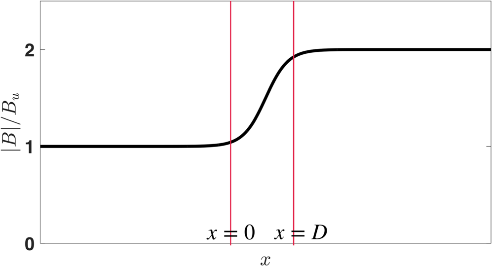
Figure 1. The magnetic field profile (schematically). The magnetic field increase occurs between $x=0$ and $x=D$
 . The region $x<0$
 is the upstream region, the region $x>D$
 is the downstream region.
3. Scattering probabilities
The probabilistic approach deals with the uniform asymptotic upstream and downstream regions where the gyrophase information is already lost and ion distributions are gyrotropic. The probabilities will be defined in the HT frame. Let a particle enter the shock with the momentum $p_i$ and pitch-angle cosine $\mu _i$
 and leave it with $p_f$
 and $\mu _f$
 . The initial and final points are in the regions where the distributions are already gyrotropic. Note that the entry and exit points may be on either side, i.e. the following scenarios are possible: (a) an ion comes from upstream and proceeds to downstream (transmission), (b) an ion comes from upstream and returns to upstream (backstreaming) and (c) and ion comes from downstream and proceeds to upstream (leakage). The option where an ion comes from downstream and returns to downstream does not exist for fast mode shocks which are considered here (Toptyghin Reference Toptyghin1980). As the initial $p_i,\mu _i$
 do not unambiguously determine the final $p_f,\mu _f$
 , we define the probability $W(\mu _i,\mu _f;p_i,p_f)$
 of scattering from the initial state to the final state as follows:

This definition is valid separately for all three types of scattering: transmission, backstreaming and leakage. Given the initial distribution $f_i(p_i,\mu _i)$ the contribution to the moments of the final distribution will take the form


If the HT frame is well-defined, the energy is conserved, $\gamma _f-\gamma _i=\text {const}$ , and $p_f=p_f(p_i)$
 is a single-valued function, so that the probability can be represented as follows:

Using the newly defined $w(\mu _i,\mu _f;p_i)$ the relation between the initial and the final distributions takes the form


where we have used the relations

In the non-relativistic regime the coefficient $C$ reduces to $C=2{\rm \pi} m^2v_iv_f$
 .
.
4. Scattering probabilities for transmitted ions in the narrow shock approximation
The main objective of the present paper is to illustrate our reformulation of the problem of the determination of the ion distribution in the simplest case where an analytical treatment is possible. We assume that the shock is planar, stationary and narrow, see figure 1. We will be treating only transmitted ions which enter the shock from upstream at $x=0$ and leave it at $x=D$
 to proceed further downstream. As the downstream region is uniform, the momentum, magnitude and pitch angle of an ion does not change any longer for $x>D$
 . Let $f(p_d,\mu _d,\varphi _d)$
 be the gyrophase-dependent distribution at $x=D$
 . From the Vlasov equation

where it is taken into account that the upstream distribution function is gyrotropic, $f_u=f_u(\mu _u;v_u)$ , and $\mu _u=\tilde {\mu }_u(\mu _d,\varphi _d;v_u)$
 is the function expressing the initial $\mu _u$
 in terms of the final $\mu _d$
 and $\varphi _d$
 . The upstream and downstream speeds are related by the energy conservation $mv_d^2/2=mv_u^2/2-q\phi _{HT}$
 . Dependence on the speed will be omitted for brevity in all calculations and restored in the end, if needed. The downstream gyrotropic distribution is obtained by the gyrophase averaging

In order to find the probability we use (3.6) with $f_i(p_i,\mu )=\delta (\mu -\mu _i)$ which gives


where the summation is over all solutions of the equation

for which the ion enters from the upstream region, $v_{u,x}>0, v_{d,x}>0$ . The coefficient $C$
 from (3.7) depends only on $v_u$
 . Thus, the problem is reduced to finding $\tilde {\mu }_u(\mu _d,\varphi _d)$
 . The equations of motion for an ion inside the shock transition are


In what follows we shall assume that all ions cross the shock without stopping inside, so that $v_x>0$ in the region $0< x< D$
 . This assumption is justified when $v_T/V_u$
 is not large and the cross-shock potential is not exceptionally high or low (Schwartz et al. Reference Schwartz, Thomsen, Bame and Stansberry1988; Dimmock et al. Reference Dimmock, Balikhin, Krasnoselskikh, Walker, Bale and Hobara2012). Ions which are reflected require special treatment. Here we restrict ourselves with the directly transmitted ions for approximate analytical treatment. Then ${\rm d}/{\rm d} t=v_x({\rm d}/{{\rm d}x})$
 and one has


The energy conservation gives

Note that (Goodrich & Scudder Reference Goodrich and Scudder1984)

In the narrow shock approximation, $D\rightarrow 0$ , one has


In what follows it will be convenient to use the normalized variables $\boldsymbol {v}/V_u$ , $\boldsymbol {B}/B_u$
 , and $s=2q\phi /mV_u^2$
 . Thus,


The remaining component of the velocity is obtained from energy conservation:


Note that a shock is essentially a discontinuity in this approximation. The corrections depending on the shock width are given in Gedalin (Reference Gedalin1997). In terms of the pitch-angle cosine one has


where $\varphi _d$ is the gyrophase of the ion at the exit point. The upstream pitch angle cosine is then


These expressions determine $\mu _u$ as a function of $v_d,\mu _d,\varphi _d$
 .
.
5. Effect of the magnetic field rotation
The dependence $\mu _u=\tilde {\mu }_u(\mu _d,\varphi _d)$ results from the global change of the magnetic field and the cross-shock potential. It is instructive to show separately the effect of the rotation of the magnetic field vector at the shock crossing, when $s_{NIF}=s_{HT}=0$
 . In this case $v_{u,x}=v_{d,x}$
 , $v_{u,z}=v_{d,z}$
 and
and


Now

and for $f_u=\delta (\mu _d\cos \varDelta + \sqrt {1-\mu _d^2} \sin \varDelta \cos \varphi _d-\mu _u)$ one has

where

The factor $1/2$ disappears because there are two solutions $\sin \varphi _d=\pm \sqrt {1-\cos ^2\varphi _d}$
 with the same absolute value. After some algebra, we find that the rotation of the magnetic field results in the scattering at the shock front described by the probability

provided


The first requirement is the condition of existence of $\phi _d$ for given $\mu _u,\mu _d$
 . The second requirement means that the ion moves toward the downstream region from the ramp and not in the opposite direction. It is obvious also that $\mu _u>0$
 , $\mu _d>0$
 . In this case $C=2{\rm \pi} m^2 v_u^2$
 .
.
6. Effect of the cross-shock potential
Analytical expressions can also be written in the narrow shock approximation for nonzero $s$ . However, they become too lengthy and difficult for qualitative understanding of the behaviour of the probabilities. Instead, we present several plots of $Cw(\mu _i,\mu _d)$
 . In the case $s_{HT}=s_{NIF}=0$
 the probability (5.8) does not depend on the speed (apart of the multiplier $C$
 ). For nonzero $s$
 this is not so. For visualization we chose $v_u=1/\cos \theta _u$
 which is the flow speed in HT frame. If the upstream distribution were cold, all ions would have this upstream speed and $\mu _u=1$
 . If the upstream thermal speed $v_T\ll 1$
 , the pitch-angle cosines remain in the vicinity of $\mu =1$
 , so that in the plots we restrict ourselves with the range $0.9\leq \mu _u\leq 1$
 , $0.9\leq \mu _d\leq 1$
 . Figure 2 shows the probability $Cw(\mu _i,\mu _d)$
 , on a logarithmic scale, for $\theta =70^\circ$
 and two values of the magnetic compression, $R=1.5$
 and $R=2.5$
 , both for zero $s$
 and nonzero $s$
 . The thin black lines in each plot correspond to the approximation of the magnetic moment conservation $(1-\mu _d^2)=R(1-\mu _u^2)$
 . It is seen that the magnetic moment is not conserved. The downstream $\mu _d$
 is no longer a single-valued function of $\mu _u$
 . The main effect is that a sudden change of the magnetic field direction immediately causes substantial gyration of an ion around the downstream magnetic field vector. The cross-shock potential reduces the ion energy and, therefore, moderates the gyration.
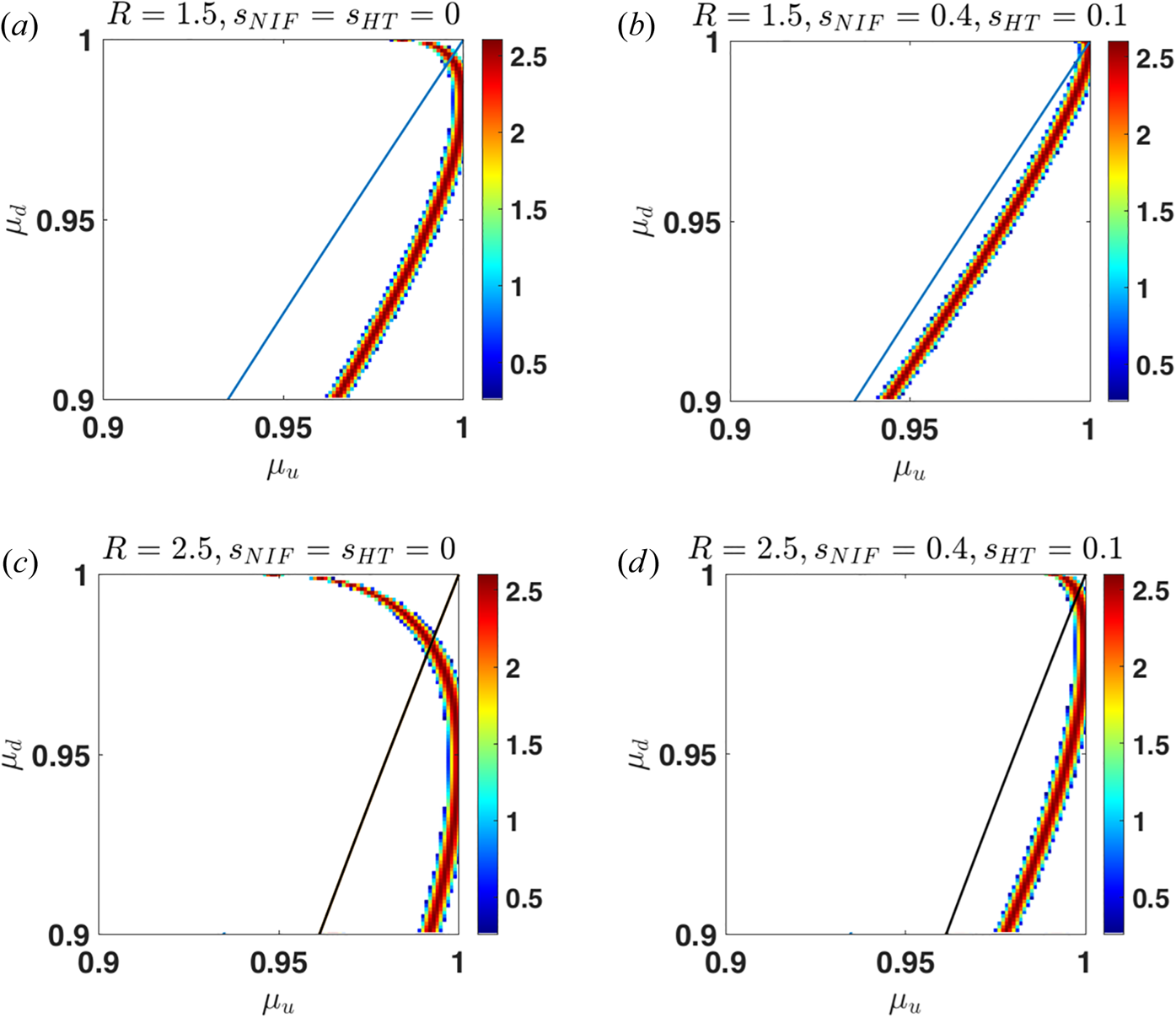
Figure 2. Filled contour plots for the probability $Cw(\mu _i,\mu _d)$ for $\theta =70^\circ$
 and four cases. For the top row $R=1.5$
 , for the bottom row $R=2.5$
 . For the left column $s_{HT}=s_{NIF}=0$
 , for the right column $s_{HT}=0,1, s_{NIF}=0.4$
 . The thin black line shows the widely used assumption of the magnetic moment conservation.
7. Conclusions
In summary, we have reformulated the problem of finding the downstream distribution function in terms of the scattering probability. This approach is not restricted to only stationary and planar shocks but can be applied to rippled and reforming shocks as well, because the scattering probabilities connect the asymptotic upstream and downstream regions, where the fields are uniform and time independent whereas the distributions are gyrotropic and also uniform and time independent. In general, finding the scattering probabilities is not an easy problem. However, they can be found numerically using test particle analysis in a model or measured shock front. When using a model no consistency of the chosen shock profile with the particle distribution is required. Indeed, the probabilities are determined by the fields upon spatial and temporal averaging. In the present paper the scattering probability of directly transmitted ions was found analytically in the limit of a narrow shock. The approach is applicable to the core of the solar wind in a planar stationary shock, even if the shock is super-critical, provided the downstream magnetic oscillations damp quickly behind the ramp (Gedalin et al. Reference Gedalin, Zhou, Russell and Angelopoulos2020). The approximation is directly applicable to laminar and nearly laminar low-Mach shocks where kinematic collisionless relaxation is observed (Balikhin et al. Reference Balikhin, Zhang, Gedalin, Ganushkina and Pope2008; Russell et al. Reference Russell, Jian, Blanco-Cano and Luhmann2009; Pope, Gedalin & Balikhin Reference Pope, Gedalin and Balikhin2019; Pope Reference Pope2020).
Acknowledgements
This work was supported in part by NASA grant 80NSSC18K1649. MG was also partially supported by the European Union's Horizon 2020 research and innovation program under grant agreement No 101004131, and by NSF-BSF grant 2019744. VR was additionally supported by NSF-BSF grant 2010144. NP was also supported by NSF-BSF grant 2010450 and by the IBEX mission as a part of NASA's Explorer program.
Editor Antoine C. Bret thanks the referees for their advice in evaluating this article.
Declaration of interests
The authors report no conflict of interest.


 Open access