2.1. (Magneto-) hydrodynamics

Solving for the motion of fluids as a function of time is a key ingredient for understanding the evolution of protoplanetary discs. Numerical hydrodynamics is a relatively mature field. Numerical solvers are either Eulerian or Lagrangian in character. Eulerian solvers trace flows across fixed discrete spatial elements, whilst Lagrangian solvers follow the motion of the flow. In protostellar disc simulations, the majority of hydro solvers are either Eulerian/Lagrangian grid-based simulators, or the fully Lagrangian Smoothed Particle Hydrodynamics.

Depending on the resolution requirements, solvers are either global, in that the entire disc extent is simulated together, or local, where a region in the disc is simulated at high resolution, with appropriate boundary conditions to reflect the surrounding disc environment. Which construction is best used is dependent upon the problem being studied, as we discuss below.

2.2. Dust–gas dynamics

The dynamics of small dust grains (Stokes number ≪ 1) is typically well coupled to that of the gas. For larger grains, however, the dust and gas dynamics can be decoupled. Properly modelling these decoupled motions is important both for disc dynamics, but also for interpreting observations. This latter point is particularly prudent given that some of the most important disc observations in recent years are millimetre continuum observations (i.e. of dust). For example, decoupled dust and gas dynamics is apparently important for understanding the symmetric gaps observed in discs (e.g. Dipierro et al. Reference Dipierro, Price, Laibe, Hirsh, Cerioli and Lodato2015b; Jin et al. Reference Jin, Li, Isella, Li and Ji2016; Rosotti et al. Reference Rosotti, Juhasz, Booth and Clarke2016).

Approaches for modelling the dynamics of dust grains that are decoupled from the motions of the gas are often distinguished by whether they use a single or two-fluid approach, both of which we discuss below.

2.3. Radiative transfer

The transport of radiation through matter is important for three primary reasons. First, radiation can modify the composition and thermal properties of matter. For example, changing the composition and heating through mechanisms such as photoionisation and photodissociation and cooling it through the escape of line emission. Radiation can also set the dust temperature, which is determined by radiative equilibrium between thermal emission from the grains and the local radiation field [there are a number of textbooks with extensive discussion of these topics, such as Spitzer (Reference Spitzer1978), Rybicki & Lightman (Reference Rybicki and Lightman1979), Osterbrock & Ferland (Reference Osterbrock, Ferland, Osterbrock and Ferland2006)]. This impact on the composition and thermal structure drives many macroscopic processes in discs (see e.g. Section 1, Figure 1). Second, radiation pressure can directly impart a force upon matter, altering the dynamics. Finally, radiation is what is actually observed. Radiative transfer is therefore required to make the most meaningful and robust comparisons between theoretical models and observations.

Since radiative transfer is fundamentally coupled to matter (influencing the composition and temperature, which in turn modifies opacities and emissivities), the coupling of radiation transport and chemistry is already an established field, which will be discussed further in Section 2.4.

For purely dynamical applications, the only quantities of interest from radiative transfer are a temperature/pressure estimate and/or a radiation pressure estimate. To this end, popular techniques are flux limited diffusion (FLD) and similar moment methods, owing to their relatively minimal computational expense compared with more detailed radiative transfer methods (e.g. Levermore & Pomraning Reference Levermore and Pomraning1981; Whitehouse & Bate Reference Whitehouse and Bate2004; Whitehouse, Bate, & Monaghan Reference Whitehouse, Bate and Monaghan2005). In FLD schemes, the directional properties of the radiation field are replaced by angle averaged ones and the radiative transfer problem is solved using a diffusion equation. FLD has long been applied in optically thick regimes without sharp density contrasts, but can generate spurious results where this is not the case (Owen, Ercolano, & Clarke Reference Owen, Ercolano and Clarke2014; Kuiper & Klessen Reference Kuiper and Klessen2013). Most modern applications of FLD account for this failure at low optical depth by using boundary conditions (e.g. Mayer et al. Reference Mayer, Lufkin, Quinn and Wadsley2007), or using hybrid methods to allow the system to radiate energy away from optically thin regions (e.g. Boley et al. Reference Boley, Durisen, Nordlund and Lord2007; Forgan et al. Reference Forgan, Rice, Stamatellos and Whitworth2009). Other approximate temperature prescriptions have also been developed that are tailored to model the effect of higher energy extreme ultraviolet (EUV) and X-ray photons from the parent star on the disc evolution (e.g. Alexander, Clarke, & Pringle Reference Alexander, Clarke and Pringle2006a, Reference Alexander, Clarke and Pringle2006b; Owen et al. Reference Owen, Ercolano, Clarke and Alexander2010; Owen, Ercolano, & Clarke Reference Owen, Ercolano and Clarke2011; Owen, Clarke, & Ercolano Reference Owen, Clarke and Ercolano2012; Haworth, Clarke, & Owen Reference Haworth, Clarke and Owen2016b).

More rigorous radiation transport methods have historically typically been confined to compute synthetic observables, where the density structure is based on snapshots from dynamical models, hydrostatic equilibrium in a simple disc, or a parametric model. Perhaps, the most popular method in this context is Monte Carlo radiative transfer (Lucy Reference Lucy1999), which is used by the well-known codes radmc-3d (Dullemond Reference Dullemond2012), mcmax (Min et al. Reference Min, Dullemond, Dominik, de Koter and Hovenier2009), hyperion (Robitaille Reference Robitaille2011), mcfost (Pinte et al. Reference Pinte, Ménard, Duchêne and Bastien2006), and torus (Harries Reference Harries2015, also discussed below). Monte Carlo radiation transport typically involves breaking the energy from radiative sources into discrete packets, which are propagated through space in a random walk akin to the propagation of real photons through matter (e.g. including scattering and absorption/re-emission events). This provides an estimate of the mean intensity everywhere which can be used, for example, to solve for the ionisation state of a gas, the dust radiative equilibrium temperature, or to generate synthetic observations. The Monte Carlo approach naturally accounts for the processed radiation field (scatterings, recombination photons), works in arbitrarily geometrically complex media and also treats multi-frequency radiation transport (conversely FLD approaches typically assume that the opacity is frequency independent).

In addition to the Monte Carlo approach, other well-known methods are also the pure (e.g. Abel & Wandelt Reference Abel and Wandelt2002) and short characteristic (e.g. Davis, Stone, & Jiang Reference Davis, Stone and Jiang2012) ray tracing schemes. Recently, intermediate expense hybrid-methods have been developed which combine FLD and other (e.g. ray-tracing) methods to offer a better balance between the accuracy of a more sophisticated scheme and the speed of FLD for dynamical applications (Kuiper & Klessen Reference Kuiper and Klessen2013; Owen et al. Reference Owen, Ercolano and Clarke2014; Ramsey & Dullemond Reference Ramsey and Dullemond2015).

2.4. Chemistry

Molecular line observations play a central role in determining both the conditions within, and kinematics of, protoplanetary discs. In particular, CO and its isotopologues are popular tracers which are relatively abundant, have a permanent dipole moment and estimates of canonical abundances in the interstellar medium (ISM). CO synthetic observations can therefore be generated relatively easily in discs by assuming the canonical abundance and that local thermodynamic equilibrium (LTE) applies, in which case the level populations are set analytically by the Boltzmann distribution (e.g. Williams & Best Reference Williams and Best2014). However, such a simple approach is not always valid. For example, in discs there is evidence of departure from the canonical CO abundance (e.g. Favre et al. Reference Favre, Cleeves, Bergin, Qi and Blake2013) and the relative abundance of isotoplogues does not necessarily scale as in the ISM (Miotello, Bruderer, & van Dishoeck Reference Miotello, Bruderer and van Dishoeck2014b). Furthermore, dust grain evolution and dynamical processes such as instabilities and planet–disc interactions can also affect the chemistry (e.g. Boley et al. Reference Boley, Durisen, Nordlund and Lord2007; Ilee et al. Reference Ilee, Boley, Caselli, Durisen, Hartquist and Rawlings2011; Evans et al. Reference Evans, Ilee, Boley, Caselli, Durisen, Hartquist and Rawlings2015; Öberg et al. Reference Öberg, Guzmán, Furuya, Qi, Aikawa, Andrews, Loomis and Wilner2015a, Reference Öberg, Furuya, Loomis, Aikawa, Andrews, Qi, van Dishoeck and Wilner2015b; Cleeves, Bergin, & Harries Reference Cleeves, Bergin and Harries2015; Huang, Öberg, & Andrews Reference Huang, Öberg and Andrews2016). Although simple CO parameterisations yield useful insights into the global properties of discs (such as the disc mass, e.g. Miotello et al. Reference Miotello, van Dishoeck, Kama and Bruderer2016; Williams & McPartland Reference Williams and McPartland2016), they are substantially more limited when it comes to probing the local properties. Given the above, more substantial chemical models will play an important role in the interpretation of modern protoplanetary disc observations. Furthermore, such models would support observations using molecules other than CO that are less easily parameterised, but could be better suited for probing certain components of a disc. In addition to interpret observations, understanding the chemical evolution of discs will also have astrobiological implications in the connection to the chemical composition of planets themselves.

To date, almost 200 molecules have been detected in interstellar or circumstellar environmentsFootnote ² . The abundances of these molecules can be subject to change via a large number of chemical reactions (see Caselli Reference Caselli, Kumar, Tafalla and Caselli2005; Henning & Semenov Reference Henning and Semenov2013, for reviews). In order to accurately model the evolution of even a small number of these molecules, complex computational networks of chemical reactions are needed in the form of coupled ordinary differential equations (ODEs). Several research groups have compiled publicly available databases of both these chemical reaction networks, and data on the rates of individual chemical reactions themselves—including the UMIST Database for AstrochemistryFootnote ³ (UDfA; Millar, Farquhar, & Willacy Reference Millar, Farquhar and Willacy1997; Woodall et al. Reference Woodall, Agúndez, Markwick-Kemper and Millar2007; McElroy et al. Reference McElroy, Walsh, Markwick, Cordiner, Smith and Millar2013), the Ohio State University networksFootnote ⁴ , and the Kinetic Database for AstrochemistryFootnote ⁵ (KIDA; Wakelam et al. Reference Wakelam2012). Databases either contain these rates explicitly, or include how such a rate depends on local properties in the form of a parameterised expression (often via the Arrhenius–Kooij equation, Arrhenius Reference Arrhenius1889; Kooij Reference Kooij1893).

Chemical reactions fall into several categories and can involve a variety of reactants. Table 1 lists the common types of astrophysical reactions. Whilst the majority of reactions are concerned with gas-phase species or their interaction with photons, dust grain surfaces provide a location for further chemistry to occur. Gas-phase molecules attach themselves to the surfaces of dust grains (a process known as adsorption) via two mechanisms: physisorption (involving weak van der Waals forces) or chemisorption (due to chemical valence bonds). Once species are adsorbed, they produce layers of ices on the surface of dust grains, which allows more complex surface chemistry to occur (Herbst & van Dishoeck Reference Herbst and van Dishoeck2009). An example of this is the process of hydrogenation, by which hydrogen reacts quickly with other surface species (including itself) to produce saturated molecules such as methane. Of particular interest for this paper is that the composition of ices on dust grains (e.g. CO-coated versus H₂O-coated) can also affect the subsequent evolution of the dust by affecting the sticking efficiency and coagulation and fragmentation efficiencies [not discussed in detail here, but see e.g. Kouchi et al. (Reference Kouchi, Kudo, Nakano, Arakawa, Watanabe, Sirono, Higa and Maeno2002), Blum & Wurm (Reference Blum and Wurm2008), Johansen et al. (Reference Johansen, Blum, Tanaka, Ormel, Bizzarro and Rickman2014); Musiolik et al. (Reference Musiolik, Teiser, Jankowski and Wurm2016), for further information]. Regions that are well shielded from incident stellar radiation (such as the disc midplane) might be thought to be chemically inert, as there is not sufficient energy to overcome reaction activation barriers. However, in such regions, ionisations caused by cosmic rays can induce ion–molecule reaction sequences that dominate much of the gas-phase chemistry, including the production of secondary cosmic-ray-induced photons. Increased densities in the disc midplane also mean that three-body reactions in the gas phase will begin to have an important effect on the chemistry. In these cases, a third body (M, the most abundant species, often molecular hydrogen) acts as a non-reacting catalyst.

Table 1. Common gas–grain reactions in astrophysical environments. Species are all considered to be in the gas phase, unless shown as X_gr, which are considered to be located on the ice mantles of dust grains. Photons are shown as γ and cosmic rays are shown as γ_cr. Adapted from Caselli (Reference Caselli, Kumar, Tafalla and Caselli2005).

In addition to (closely coupled to) the computation of abundances is the computation of the temperature. This is determined by the heating and cooling rates, which are themselves set by, to name just a few: radiative processes (e.g. photoionisation heating and line cooling), dust/PAH’s (e.g. PAH heating and grain radiative cooling), chemical processes (e.g. exothermic reactions), hydrodynamic work/viscous heating, and cosmic rays (a review is given by Woitke Reference Woitke, Kamp, Woitke and Ilee2015). Many of these heating/cooling terms are linked to the composition of the gas, requiring chemical and thermal calculations to be solved iteratively. In principle, since the heating and cooling is also set by the dust and radiation field, it might also be necessary to iterate over the (decoupled dust–gas) dynamics and radiative transfer.

Somewhat distinct from gas–grain chemistry are the photoionisation and photon-dominated region (PDR) regimes, where the radiation field plays a significant role in setting the composition and temperature of a medium. Photoionised gases are composed exclusively of atoms and ions and are typically modelled more in a radiative transfer context than a chemical one. Photoionisation models are usually concerned with the transfer of EUV photons and X-rays to solve for the ionisation balance and thermal structure of a gas of assumed gas and dust abundances. Despite not requiring chemical networks, this can include a variety of processes that are not trivially captured such as resonant line transfer and inner shell ionisations of atoms by X-rays (the liberation of multiple electrons by a single photon). Some examples of famous photoionisation codes are cloudy (Ferland et al. Reference Ferland2013) and mocassin (Ercolano et al. Reference Ercolano, Barlow, Storey and Liu2003). The photoionised regime only applies to disc winds, the very surface layers/inner edge of discs and, if the disc is externally irradiated by high energy photons (e.g. from a nearby O star), components of the flow from the disc outer edge.

The PDR regime applies at the transition between photoionisation and gas–grain dominated regimes; between predominantly ionised and molecular gasses. For example, in surface layers of the disc, but generally wherever matter is not optically thick to far ultraviolet (FUV) radiation. PDR modelling, like the gas–grain regime, requires a chemical network to be solved. It is also further complicated because cooling by line photons can be very important. This means that although the local radiation energy density (exciting the gas) is a single parameter, the escape probability of the line photons depends upon the extinction in all directions, i.e. it depends on the 3D structure of the surrounding space. Many PDR codes therefore compute this escape probability in one direction only, either working in 1D (e.g. models such as those in Röllig et al. Reference Röllig2007) or making some assumption about the dominant direction (e.g. vertically in the disc). Of the latter type, so called 1+1D models are particularly popular, which assume that at any given radial distance from the sta, the disc is in hydrostatic balance and escaping photons only consider the vertical distribution of gas at that radius (e.g. Gorti, Dullemond, & Hollenbach Reference Gorti, Dullemond and Hollenbach2009; Woitke et al., Reference Woitke2016). Recently, multi-dimensional numerical approaches to solving PDR chemistry have appeared that do compute the 3D escape probabilities (Bisbas et al. Reference Bisbas, Bell, Viti, Yates and Barlow2012, Reference Bisbas, Haworth, Barlow, Viti, Harries, Bell and Yates2015b) which they do efficiently using healpix (Górski et al. Reference Górski, Hivon, Banday, Wandelt, Hansen, Reinecke and Bartelmann2005).

2.4.1. Remarks on chemistry and radiative transfer

Chemical networks are used in conjunction with radiative transfer models to compute chemical abundances in various astrophysical environments. In general, the abundances are functions of temperature, density, and local radiation field, though many other parameters can play a role (in particular in the regime where line cooling is important, a measure of the extinction in all directions is ideally required). Often, the chemical networks are integrated to equilibrium in regions where the physical conditions are not thought to change significantly with time. However, in many cases, the microphysical conditions are functions of both space and time and are therefore not independent of dynamical processes (an example of this is given in Figure 3, see also Boley et al. Reference Boley, Durisen, Nordlund and Lord2007; Ilee et al. Reference Ilee, Boley, Caselli, Durisen, Hartquist and Rawlings2011; Evans et al. Reference Evans, Ilee, Boley, Caselli, Durisen, Hartquist and Rawlings2015; Drozdovskaya et al. Reference Drozdovskaya, Walsh, van Dishoeck, Furuya, Marboeuf, Thiabaud, Harsono and Visser2016).

Figure 3. Left: The three-dimensional evolution of a tracer particle in a self-gravitating disc, colour coded with temperature changes, overlaid on the final column density snapshot of the disc. Right: The corresponding chemical evolution of particle, showing gas-phase CO and H₂CO, and CO ice (gCO). The shocks induced by the self-gravity of the disc have a significant impact on the chemical composition of the disc material (see Boley et al. Reference Boley, Durisen, Nordlund and Lord2007; Ilee et al. Reference Ilee, Boley, Caselli, Durisen, Hartquist and Rawlings2011; Evans et al. Reference Evans, Ilee, Boley, Caselli, Durisen, Hartquist and Rawlings2015).

Recent work has seen an increase in performing chemical evolution calculations alongside the radiative transfer calculations (e.g. Bruderer, Doty, & Benz Reference Bruderer, Doty and Benz2009; Woitke, Kamp, & Thi Reference Woitke, Kamp and Thi2009). Furthermore, chemistry is now being coupled directly with hydrodynamic calculations: In the context of star-forming regions, there are the full hydrodynamic models of Glover et al. (Reference Glover, Federrath, Low and Klessen2010) and in a 1+1D disc framework, there are models such as those by Gorti et al. (Reference Gorti, Dullemond and Hollenbach2009) which also include radiative transfer. Such coupling is particularly important in the regions of the discs where the gas is not thermally coupled to the dust (i.e. in the upper layers of the disc, or within the dust sublimation radius), since the gas temperature, gas abundances, and level populations are strongly correlated. Unfortunately, it is in these regions of importance that 1+1D models become less applicable due to deviations from hydrostatic equilibrium (for example, thermally driven winds are not hydrostatic, e.g. Clarke & Alexander Reference Clarke and Alexander2016). Dynamically, some chemical regimes (in particular, the PDR regime) are definitely important for understanding certain processes. For example, PDR physics is required to model FUV driven photoevaporative flows from the outer edge of discs (Adams et al. Reference Adams, Hollenbach, Laughlin and Gorti2004; Facchini et al. Reference Facchini, Clarke and Bisbas2016; Haworth et al. Reference Haworth, Boubert, Facchini, Bisbas and Clarke2016a). The dynamical importance of gas–grain chemistry in cooler regions of the disc is currently yet to be determined, for example, presently unidentified chemically induced dynamical instabilities could potentially arise (see the burning questions, Section 3.1).

Aside from the coupling of chemistry with new physics such as dynamics, it is very important to stress that our base understanding of astrochemistry is constantly and rapidly evolving, with new species, reactions, and regimes being identified that can only be studied in a dedicated manner [for example, Penteado et al. (in preparation) use 10 000 models to study the sensitivity of single point chemical models to bind energies]. It is important that such focussed study continues.

Considering again the dust, there is no obvious consensus at present as to the best way to perform self-consistent dusty radiation hydrodynamics calculations of protoplanetary disc evolution. Schemes such as the short characteristics Variable Eddington Tensor (VET) method implemented in the Athena code by Davis et al. (Reference Davis, Stone and Jiang2012), or the hybrid approach by Kuiper & Klessen (Reference Kuiper and Klessen2013) show promise for bridging the gap between FLD and ray-tracing, but still require accurate modelling of the small grain dust population to determine the opacities before they can be applied in the context of protoplanetary discs (see Section 2.2).

With respect to magnetic fields, there are now also some approaches capable of modelling both radiation and MHDs (e.g. Flock et al. Reference Flock, Fromang, González and Commerçon2013; Tomida, Okuzumi, & Machida Reference Tomida, Okuzumi and Machida2015).

Based on the above, we are already making excellent progress in cross-disciplinary modelling of discs, but most of this progress is very recent. There are still a number of highly coupled processes that cannot yet be modelled. As we will now discuss, there is a long, but fruitful journey ahead of multi-physics disc modellers.

3.1. Burning questions

Some examples of ‘burning’ science questions raised either during our discussion sessions, or by members of the community commenting on this paper, which might motivate improved multi-physics modelling of discs, included:

• • What are the main drivers of global disc evolution? In particular, what is the main driver of the mass accretion rate in protoplanetary discs?

• • Alongside magnetic fields, what other processes govern or control the launching of jets and outflows?

• • What is the effect of environment on protoplanetary disc evolution? For example, discs close to O stars are clearly heavily disrupted by high energy photons (we observe such systems as proplyds), but what is the role of comparatively modest radiation fields?

• • Do chemical–dynamical instabilities exist, i.e. is there a chemical reaction that feeds back into the dynamics (e.g. thermally) but responds to the dynamical change with a faster reaction rate?

• • What happens to small grains at the surface of the disc or in outflows/winds?

• • What happens at high dust to gas ratios? How important are streaming instabilities, or other instabilities? How important are self-induced dust traps? What happens to dust in shocks?

• • How do magnetic fields in the disc affect the behaviour of charged dust grains, and how do the dynamics and ionisation chemistry of the grain population in turn affect the magnetic field evolution?

• • What are the conditions under which pebble accretion (e.g. Ormel & Klahr Reference Ormel and Klahr2010; Lambrechts & Johansen Reference Lambrechts and Johansen2012; Morbidelli & Nesvorny Reference Morbidelli and Nesvorny2012) might operate, and how will this impact the diversity of planetary systems formed in protoplanetary discs (e.g. Bitsch, Lambrechts, & Johansen Reference Bitsch, Lambrechts and Johansen2015; Chambers Reference Chambers2016; Ida, Guillot, & Morbidelli Reference Ida, Guillot and Morbidelli2016)?

• • What is the nature of fragmentation in self-gravitating discs? Is there a well-defined parameter space where fragmentation occurs (c.f. Meru & Bate Reference Meru and Bate2011; Michael et al. Reference Michael, Steiman-Cameron, Durisen and Boley2012; Rice, Forgan & Armitage Reference Rice, Forgan and Armitage2012; Rice et al. Reference Rice, Paardekooper, Forgan and Armitage2014), or can it occur stochastically through rare high-amplitude density perturbations over long enough timescales (Paardekooper Reference Paardekooper2012; Young & Clarke Reference Young and Clarke2016)?

• • What is the origin of rings, gaps, horseshoes, and cavities observed in mm-continuum emission? How common are these features?

• • How can the masses and properties of embedded protoplanets be constrained from observations?

• • How do planets affect observations of chemical tracers?

• • How do planets and circumplanetary discs affect the evolution of the protoplanetary disc (e.g. through thermal feedback or increased radiative heating in gaps). Conversely, how does the disc affect an embedded planet (e.g. the planetary atmosphere).

• • Will dust discs fragment?

• • What determines the scale height of the dust layer? How is this set by different processes, for example, coagulation (e.g. Krijt & Ciesla Reference Krijt and Ciesla2016)?

• • Under which conditions do warps develop in discs? Can radiation pressure drive warping?

• • What are the possible initial conditions of class I/II/III discs and how do they influence the subsequent evolution? In particular, how does the early evolution of discs affect the chemistry and grain distribution (e.g. Miotello et al. Reference Miotello, Testi, Lodato, Ricci, Rosotti, Brooks, Maury and Natta2014a)? What is inherited from the star-formation process?

• • The vertical component of the magnetic field controls the mass flux of winds and the saturation level of MRI-driven turbulence. How does the competition between accretion (drawing the vertical field in towards smaller radii) and diffusivity (pushing it outwards towards larger radii) cause this component of the field to vary with time? In particular, what is the magnitude of the diffusivity term, which is set by microphysics (e.g. Lubow, Papaloizou, & Pringle Reference Lubow, Papaloizou and Pringle1994; Rothstein & Lovelace Reference Rothstein and Lovelace2008; Takeuchi & Okuzumi Reference Takeuchi and Okuzumi2014)?

• • How turbulent are protoplanetary discs (e.g. Flaherty et al. Reference Flaherty, Hughes, Rosenfeld, Andrews, Chiang, Simon, Kerzner and Wilner2015; Simon et al. Reference Simon, Hughes, Flaherty, Bai and Armitage2015a; Teague et al. Reference Teague2016)?

• • What is the process by which a protoplanetary disc becomes a debris disc? Transition discs; those with inner holes, are typically attributed to the action of photoevaporation by the host star (see e.g. Owen Reference Owen2016), or planets (e.g. Zhu et al. Reference Zhu, Nelson, Hartmann, Espaillat and Calvet2011). But which, if either, of these is the dominant process [examples of models including both are Alexander & Armitage (Reference Alexander and Armitage2009), Rosotti, Ercolano, & Owen (Reference Rosotti, Ercolano and Owen2015)]? Are there other processes that contribute significantly to disc dispersal, such as magneto-thermal winds (Bai et al. Reference Bai, Ye, Goodman and Yuan2016)? What are the initial conditions of debris disc models (e.g. Takeuchi, Clarke, & Lin Reference Takeuchi, Clarke and Lin2005; Thilliez & Maddison Reference Thilliez and Maddison2015)?

Some of these questions might only be addressed by combining all of the physical ingredients of protoplanetary disc modelling. However, several will only require consideration of a smaller fraction. These smaller steps will be extremely valuable in bridging the gaps between fields, and will undoubtedly inform the production of a fully comprehensive modelling approach. We manifest these steps as a series of challenges, outlined below.

3.2. Grand challenges for gas modelling

3.3. Grand challenges for dust–gas modelling

Simultaneously compute the dynamics and size evolution of the entire grain population, coupled to self-consistent modelling of the gas and radiation field in the disc in global, 3D simulations. This can be broken into a series of smaller challenges, as follows:

4.1. Which problems are the most pressing to solve and what physics is required to solve them?

It is inefficient to develop new software, or exhaust substantial CPU hours on an intensive state of the art multi-physics calculation, if the results have no value. A key strategic step, therefore, is to identify the combination of physics required to answer well motivated, well formulated, key problems.

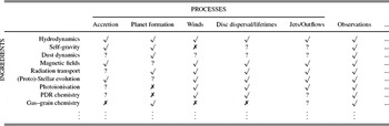
Table 2 provides an example of a strategic overview. Such an overview can guide/motivate the development of numerical methods to include all of the physics essential to solve a given problem. It would also motivate us to understand whether the uncertain features really do play an important role.

Table 2. A qualitative summary of the effect of different components of disc modelling on the intrinsic physical properties of protoplanetary discs – ‘✓’ implies that an ingredient is identified as important, ‘?’ implies that the importance is uncertain, ‘✗’ implies that an ingredient is likely unimportant. It is our hope that such a summary would eventually become more quantitative, with the relative importance of different processes more formally assessed.

In addition to identifying the processes that might contribute to a problem (such as in Table 2), one could possibly then order the contributing physical processes in a hierarchy of importance to determine which are the most important features to include in a model (similar to the way that the dynamical importance of microphysics on H ii region expansion was categorised by Haworth et al. Reference Haworth, Harries, Acreman and Bisbas2015). For example, consider the generation of synthetic molecular line observations. At the most basic level radiative transfer is required, as it is photons that are observed by astronomers, as well as some estimate of the density, temperature, molecular abundance, and molecular level populations. This can initially be done assuming some simple static disc structure, assuming an abundance of molecules and level populations determined analytically by the Boltzmann distribution. This could then be improved with proper non-local thermodynamic equilibrium (NLTE) statistical equilibrium calculations, which could be improved upon by using chemical networks/direct abundance calculations, which can be improved upon by further solving the dynamics/thermal balance, decoupled dust transport, and so on. In order to do this, one would first need to define some measure of importance. For example, if interested in accretion, a hierarchy of importance would place processes resulting in the largest contribution to the accretion rate at the top.

Deciding which problems are most pressing to address should also be informed by recent and upcoming observations. For example, which questions might be addressed by models in tandem with data from the Square Kilometer Array [SKA, which amongst other things will probe grain growth and disc chemistry (Testi et al. Reference Testi2015)], James Webb Space Telescope (JWST) or the European-Extremely Large Telescope (E-ELT, e.g. Hippler et al. Reference Hippler, Usuda, Tamura and Ishii2009)?

Another key strategic point is to stress that on the path towards multi-physics modelling of significantly interdependent physics, it is essential that all individual fields continue to develop as they are presently. Integration should be complementary to our current approaches. There are (at least) two key reasons for this. One reason is that an integrated approach is likely to be substantially more computationally expensive, which limits the parameter space of a given problem that can be studied. This also strongly limits the ability to quickly interpret observations (e.g. with parametric models). The other reason is that each field is continuing to evolve, with the development of new algorithms and the identification of new important mechanisms. This focussed field-by-field progression will likely answer a number of the burning questions and the techniques developed will ultimately feed back into multi-physics models of the future.

5.1. Simplified chemistry for dynamics

We currently identify three possible approaches to include chemistry in dynamical simulations: direct calculation of a full network and heating/cooling rates, direct calculation of a reduced network, or implementation of pre-computed look-up tables. We discuss these further below.

5.2. Direct hybridisation

Historically, the approach to include more physics in dynamical models is to use a hydrodynamical code as the foundation and incorporate simplified physics modules subsequently. For example, Glover et al. (Reference Glover, Federrath, Low and Klessen2010) and Dzyurkevich et al. (Reference Dzyurkevich, Commerçon, Lesaffre and Semenov2016) patch reduced chemical networks into zeus-mp and ramses, respectively. Flock et al. (Reference Flock, Fromang, González and Commerçon2013) also present an extension of the pluto code that includes both magnetic fields and an FLD radiation transport scheme. There is another approach, which is to start with a state of the art chemistry/radiative transfer code and subsequently incorporate somewhat more simple hydrodynamics. An example of this latter approach is the torus radiation transport and hydrodynamics code. This code began its life solely as a Monte Carlo radiative transfer code (Harries Reference Harries2000) but now includes hydrodynamics, so can perform radiation hydrodynamic simulations with all the features of a dedicated radiation transport code (e.g. detailed photoionisation, dust radiative equilibrium, and radiation pressure in arbitrarily complex system geometries, etc.; Haworth & Harries Reference Haworth and Harries2012; Harries Reference Harries2015; Haworth et al. Reference Haworth, Harries, Acreman and Bisbas2015). Furthermore, torus-3dpdr is an extension of torus that also includes PDR chemistry with 3D extinction and escape probabilities (Bisbas et al. Reference Bisbas, Haworth, Barlow, Viti, Harries, Bell and Yates2015b). The UV radiation field everywhere is computed using the Monte Carlo radiation transport and the escape probabilities are estimated in 3D using an algorithm based on healpix (Górski et al. Reference Górski, Hivon, Banday, Wandelt, Hansen, Reinecke and Bartelmann2005). torus-3dpdr is capable of directly modelling the role of FUV photons dynamically in non-hydrostatic scenarios, such as the external irradiation of discs by FUV radiation that has only been possible semi-analytically in the past (Adams et al. Reference Adams, Hollenbach, Laughlin and Gorti2004; Facchini et al. Reference Facchini, Clarke and Bisbas2016; Haworth et al. Reference Haworth, Boubert, Facchini, Bisbas and Clarke2016a). It could also be used to test the validitiy of escape probability methods that assume a single dominant trajectory (the 1+1D methods).

One argument in favour of adding hydrodynamics to a radiative transfer/chemistry code is development time, since a simple but effective hydrodynamics algorithm is usually much more straightforward to develop than a radiative transfer/chemistry algorithm (though of course care must be taken to ensure that the hydrodynamics algorithm is appropriate for any given application). The obvious argument against this coupling of state of the art physics models with hydrodynamics is that they are not necessarily well streamlined and can be very computationally expensive (though this is not necessarily a problem if the code is optimised and/or highly scalable, as is the case for torus, Harries Reference Harries2015).

Constructing a dedicated photochemical-dynamical code from scratch is another possible option, but potentially requires a lot of development time (e.g. the recent PDR-dynamical code of Motoyama et al. Reference Motoyama, Morata, Shang, Krasnopolsky and Hasegawa2015).

Another promising avenue is the development of diverse, flexible self-consistent physics libraries that can be ported into other numerical (and therefore potentially hydrodynamical) codes. The krome code is an excellent example of this approach, which quickly solves arbitrary chemical networks and can also calculate heating and cooling terms (Grassi et al. Reference Grassi, Bovino, Schleicher, Prieto, Seifried, Simoncini and Gianturco2014). Spectral codes, which solve partial differential equations flexibly and efficiently, could also offer a powerful means of combining other physical ingredients in a relatively straightforward manner. Spectral codes appear not to have featured in multi-physics disc modelling to date, but options for doing so include the dedalus (Burns et al. Reference Burns, Brown, Lecoanet, Oishi and Vasil2016) and snoopy (Lesur Reference Lesur2015) codes.

5.3. Temporal and spatial resolution

A very specific problem is that (in particular for non-equilibrium chemical-dynamics) we have to determine what the spatial and temporal scales are that we have to resolve in a given scenario. As an example, chemical timescales in the disc upper layers (that is, in the PDR regions) are rather short, whereas timescales deeper in the disc are usually much longer (for example, the case of CO being converted into CH₄ on timescales even longer than protoplanetary discs lifetimes). The time steps required to model the upper layers may therefore eventually be limited by the chemical timescales (in non-equilibrium scenarios) rather than the dynamical timescales, which might drastically increase computational expense. In such a regime where the chemical timescale is very small (much smaller than the dynamical timescale), we may be able to alleviate the problem somewhat with chemical sub-stepping—running multiple chemical updates per hydrodynamic update. Conversely, if the chemical/thermal timescales (reaction/heating/cooling rates) are very long, many dynamical steps can be taken between the more expensive chemical updates, improving the computation time substantially.

Alternatively, if the system is expected to reach a steady state, and all that is desired is an accurate model of this steady state (rather than the pathway to reaching the steady state), it may be possible to run chemical calculations very infrequently even if the chemical timescale is very short.

In addition to the above timescale arguments, resolution also needs to be considered. For example, some chemical features may only arise if the spatial resolution (e.g. around shocks) is sufficiently high—capturing such processes will of course increase computational expense.

5.4. Scaling

A key technical consideration is the scaling of the various physical ingredients in terms of both elements (cells, rays, chemical species, reactions, etc.) and computational resources (number of cores), since a calculation is going to be limited by its least tractable component. Different numerical approaches to computing a given ingredient can scale very differently. For example, in the case of radiative transfer, Monte Carlo radiation transport and treecol (see Clark, Glover, & Klessen Reference Clark, Glover and Klessen2012, for details of the latter) scale much more efficiently than long characteristic ray tracing. There are therefore multiple scaling options per ingredient.

For applications comprising two or more ingredients that scale very differently, there will likely be idle cores/inefficient CPU usage in the components of the code that do not scale so well. Furthermore, some techniques have specific constraints on the number/configuration of cores which may vary for different calculation ingredients. For example, if the hydrodynamic component of a calculation were confined to i distributed memory MPI threads (plus an arbitrary number of shared memory openMP threads), but the radiative transfer to j > i MPI threads, there will be unused MPI threads during each hydrodynamics step. This is a situation where dynamically optimising between shared and distributed memory processes is worthwhile, setting the otherwise idle MPI threads to contribute to openMP or other useful tasks.

5.5. Hardware developments

It is also important to assess new and projected hardware developments. We are approaching a time in which access to large numbers of processors increasingly outweighs the developments in performance of the processors themselves. Efficiently scalable numerical methods, such as Monte Carlo radiation transport and discontinuous Galerkin hydrodynamics solvers, will therefore be extremely advantageous in the near future.

Another significant realisation (only recently for astronomers) is that graphics processing units (GPUs) can offer significant speedup per core. A relatively small (but growing) fraction of astrophysical codes have a GPU implementation, and those that do are often those used for cosmological applications (e.g. Schive, Tsai, & Chiueh Reference Schive, Tsai and Chiueh2010; Bryan et al. Reference Bryan2014b). However, a GPU implementation of the fargo disc-modelling code was developed by Benítez-Llambay & Masset (Reference Benítez-Llambay and Masset2016), where they quote a typical speedup per core of a factor 40. It is beyond the scope of this paper to discuss GPU programming in detail, but we note that GPUs are fundamentally different architectures to CPUs and are therefore programmed in a somewhat different manner (taking time to learn), typically using either the cuda (Nickolls et al. Reference Nickolls, Buck, Garland and Skadron2008) or opencl (Stone, Gohara, & Shi Reference Stone, Gohara and Shi2010) standards. The high speeds of GPUs make them a powerful tool for the future of astronomy, where applicable, and they are likely to feature much more frequently in astronomy in the coming years, especially with the advent of directive-based GPU acceleration using the OpenACC standardFootnote ⁶ .

A final example, mentioned here only in passing, is the introduction of new types of processor such as the Intel Xeon Phi (e.g. Jeffers & Reinders Reference Jeffers and Reinders2013)—which combines some of the performance advantages of GPUs with an easier programming framework.

In general, the writing of new codes, or adapting old ones, to take advantage of hardware developments will be important. Given that more specialised hardware might continue to appear over time, it would also be advantageous if codes could be developed in such a fashion that they are easily ported, but it is unclear (to us at least) exactly how this might work in practice. This is an area where increased collaboration between astrophysicists and computer scientists will be advantageous. Interaction with computer scientists could also lead to other benefits such as improved efficiency of our codes and the promotion of better coding practice.

6.1. Workshops

Workshops are likely to be essential for stimulating cross-disciplinary collaboration. Whilst a typical conference setting will be important for each sub-discipline to discuss their work generally, events with ample time for break-out sessions and collaborative spaces are likely to be very productive. Such events allow large-scale discussion, but also allow for specific problems to be tackled one-on-one or in small groups in an ‘unconference’ setting (for example, the dotAstronomyFootnote ⁷ or AstropyFootnote ⁸ conference series). The identification of key ingredients to be swapped between respective fields will be important to establish, e.g. heating and cooling rates are likely to be of interest to those running dynamic models, whilst detailed abundance results may not be required.

6.2. Benchmarking

In addition to workshops, it is important for each field to develop an agreed set of benchmark problems, with the aim of transparency and reproducibility. Code comparison projects are key, but can require a lot of work for a small number of publications (albeit high impact, e.g. de Val-Borro et al. Reference de Val-Borro2006; Röllig et al. Reference Röllig2007; Pinte et al. Reference Pinte, Harries, Min, Watson, Dullemond, Woitke, Ménard and Durán-Rojas2009; Iliev et al. Reference Iliev2009).

A good example of a successful comparison project is the recent StarBench code comparison workshopsFootnote ⁹ (Bisbas et al. Reference Bisbas2015a). These workshops aimed at testing radiation hydrodynamics codes used to study problems in star formation, with an emphasis on doing so in a positive and friendly environment. The workshops involved attendees running tests before arrival, which spanned a range of complexity. In the first meeting at the University of Exeter in 2013, every code passed the purely hydrodynamic shock tests without issue. However, the instant that radiative transfer/photoionisation was introduced into the dynamical problem we generally had poor agreement, even for the simplest case of tracking the time evolution of the extent of an ionised region about a star in a uniform density medium composed solely of hydrogen. The origin of the inconsistency between codes was that they were all running slightly different models (e.g. inconsistent recombination rates) and, after extremely careful rewriting of the specifications of this simple test, were subsequently able to get truly excellent agreement between the codes. This process highlighted to the community all of the things that should be explicitly stated in a paper in order to make it truly reproducible. Last but not least, in the case of an expanding H ii region, we actually discovered that although the codes all agreed perfectly, they did not agree with the classic analytic solution that everyone would compare with in their numerical methods paper and suggest that they get ‘good enough’ agreement with—validating their approach. Following re-investigation, as a result of code comparison, a direct improvement in our understanding of this fundamental analytic problem has been established (Bisbas et al. Reference Bisbas2015a). In summary, code comparison

• • verifies that codes are working as desired;

• • informs the community what needs to be specified in papers to make them reproducible—a key factor, especially since there are likely to be many more ingredients in disc models of the future than there were in the relatively straightforward StarBench tests;

• • improves our understanding of each other’s numerical methods, including relative strengths and weaknesses. This can be done in a friendly way;

• • highlights the importance of careful numerics (e.g. understanding resolution dependency and which techniques are appropriate for a given scenario);

• • results in high impact publications;

• • leads to an improvement in our understanding of the underlying more fundamental (even analytic) problems.

Key to a successful comparison is active feedback between participants and iteration towards understanding the origin of any differences encountered. This can often be achieved just as easily with a comparison involving just two or three codes performed by a relatively small team (e.g. Bate & Burkert Reference Bate and Burkert1997; Commerçon et al. Reference Commerçon, Hennebelle, Audit, Chabrier and Teyssier2008; Price & Federrath Reference Price and Federrath2010; Hubber, Falle, & Goodwin Reference Hubber, Falle and Goodwin2013). Such an approach avoids much of the friction associated with large-scale comparison projects whilst achieving the same objectives.

6.3. Open source software

A more applied collaborative practice is to develop software in an open source format (e.g. using GitHubFootnote ¹⁰ ). This is potentially very useful for both transparency and distributed development (i.e. international contributors). Examples taking such an approach are the krome (Grassi et al. Reference Grassi, Bovino, Schleicher, Prieto, Seifried, Simoncini and Gianturco2014) and lime (Brinch & Hogerheijde Reference Brinch and Hogerheijde2010) projects.

Although the open source mentality is desirable, it should not be imposed since there may be legitimate reasons to protect intellectual interests. For example, if an early-career researcher invests substantial time into code development, the current academic culture requires a period where they are able to see a return on their time investment, in terms of first author publications where they lead astrophysical research (in the current culture, this is more important than a number of co-authored publications). There is no reason that their code cannot be shared collaboratively during such a phase of research. More widespread access can subsequently be yielded once the developers have seen sufficient return.