


1. Introduction
Annuity providers, such as insurers and pension funds, are exposed to increased longevity risk. This risk can be broken down into two types of risks: unsystematic and systematic. Unsystematic longevity risk refers to a possible adverse development of the policyholder’s longevity. According to the law of large numbers, unsystematic longevity risk can be eliminated by increasing the portfolio size. In contrast, systematic longevity risk refers to the risk associated with the overall mortality improvement across the whole population. This risk cannot be diversified by increasing the portfolio size but can be mitigated by entering longevity-linked securities, such as survivor bonds, q-forwards, S-forwards or S-swaps (Blake and Burrows, Reference Blake and Burrows2001; Dowd et al., Reference Dowd, Blake, Cairns and Dawson2006; Barrieu and Veraart, Reference Barrieu and Veraart2014; Levantesi and Menzietti, Reference Levantesi and Menzietti2017 and Zeddouk and Devolder, Reference Zeddouk and Devolder2019). Some of these financial instruments have been traded over the counter (OTC), but because of pricing difficulties and the fact that these products only allow for partial hedging of the systematic longevity risk (leaving a residual amount of risk, known as basis risk), they are not widely traded in the financial market. The payoffs of these financial instruments are determined by longevity indices based on one or more reference populations (e.g., the national population). Therefore, the longevity experience of the annuity provider’s population may not coincide with the reference population (see for example Li and Hardy, Reference Li and Hardy2011 and Coughlan et al., Reference Coughlan, Khalaf-Allah, Ye, Kumar, Cairns, Blake and Dowd2011).
The importance of the basis risk induced by the mismatch between the reference population and the insurer’s population depends on different factors, such as demographic differences (e.g., age profile, sex, socio-economic status), the volatility of the portfolio to be hedged in comparison with the reference population and the difference between the payoff structures of the hedging tool and the insurer’s portfolio (Li et al., Reference Li, Li, Tan and Tickle2019).
Many authors have focused on the evaluation of the basis risk. For instance, De Rosa et al. (Reference De Rosa, Luciano and Regis2017) provided a model for assessing longevity basis risk, exploring its effect on the hedging strategies of pension funds and annuity providers. Haberman et al. (Reference Haberman, Kaishev, Millossovich, Villegas, Baxter, Gaches, Gunnlaugsson and Sison2014) and Villegas et al. (Reference Villegas, Haberman, Kaishev and Millossovich2017) proposed a two-population mortality projection model for assessing demographic basis risk. Additionally, Plat (Reference Plat2009) proposed a stochastic model for the spread between reference and the smaller population that allowed insurers to evaluate mortality rates and assess the basis risk; Cairns and El Boukfaoui (Reference Cairns and El Boukfaoui2021) developed a framework for measuring the impact of a hedge on regulatory or economic capital that considered basis risk (see also Coughlan et al., Reference Coughlan, Khalaf-Allah, Ye, Kumar, Cairns, Blake and Dowd2011; Dahl et al., Reference Dahl and Glar2011; Li and Hardy, Reference Li and Hardy2011; Ngai and Sherris, Reference Ngai and Sherris2011; Tzeng et al., Reference Tzeng, Wang and Tsai2011, and Li and Luo, Reference Li and Luo2012).
Specifically, Zhou and Li (Reference Zhou and Li2017) presented the basis risk as a “customised surplus swap” in addition to standardised financial instruments. However, the management and the pricing of this swap are based on mutualisation and reinsurance’s classical principles without a risk premium (diversification argument) or references to financial valuation.
The main contribution of our paper is to extend this approach by associating the basis risk with the payoff of a longevity-linked OTC security, called S-exchange. We price this derivative under Solvency II using the cost of capital (COC) approach in a continuous time framework. Thus, we liken this basis risk to the S-exchange, whose price corresponds to the hedging cost of this risk.
To achieve this goal, we developed a model capable of describing the mortality of the reference and the insurer’s populations. Many authors have proposed stochastic multi-population models for mortality, such as Bayraktar and Young (Reference Bayraktar and Young2010), Barbarin (Reference Barbarin2008) and Dahl et al. (Reference Dahl and Melchior2008). Moreover, some continuous-time models such as the general multi-population mortality surface model proposed by Jevtié and Regis (Reference Jevtić and Regis2019) and the multi-cohort models used by De Rosa et al. (Reference De Rosa, Luciano and Regis2017) and Sherris et al. (Reference Sherris, Xu and Ziveyi2020) have emerged recently.
Our mortality model needed not only to forecast mortality but also to enable the valuation of longevity derivatives. Therefore, affine models are good candidates because they meet these criteria (Huang et al., Reference Huang, Sherris, Villegas and Ziveyi2019 and Xu et al., Reference Xu, Sherris and Ziveyi2020). In addition to their proven robustness in terms of mortality prediction (Luciano and Vigna, Reference Luciano and Vigna2015, and Zeddouk and Devolder, Reference Zeddouk and Devolder2020a), affine models have the advantage of facilitating the pricing of longevity derivatives and enabling the adoption of the pricing framework developed in finance for the valuation of financial assets. Thus, we used a one-cohort affine model that we redesigned into a multi-population model.
Specifically, we used the Hull and White (HW) process in our framework to provide different multi-population models, depending on eventual differences between the reference population and the insurer’s population.
Our other contribution consists in providing fair prices for the proposed hedging instrument (in closed form when possible), using the COC method, which aligns with the directives of Solvency II. In addition, we used other classical pricing approaches for comparison. Then, depending on the insurer’s strategy and risk aversion, we provided different hedging options using longevity derivatives. The modelling and pricing framework proposed in this paper offer hedgers various strategies to reduce or completely cover their exposure to longevity risk.
This paper is organised as follows: In Section 2, we propose a multi-population model to describe mortality for the reference and insurer’s population. In Section 3, we briefly define the S-forward contract and its pricing, then in Section 4, we define the S-exchange contract and provide closed-form formulas of its price under some classical financial pricing approaches, as well as the COC approach. In Section 5, we investigate three special cases to model the insurance population’s mortality. Then, in Section 6, we present a numerical illustration of the prices using Belgian data. We provide sensitivity tests related to the different parameters in Section 7 and propose different longevity hedging strategies in Section 8. Finally, Section 9 concludes the paper.
2. Multi-population modelling in continuous time
In order to assess the basis risk, we need to use a model able to capture mortality trends in both the reference population and the insurer’s population, whose risk is to be hedged. We model mortality for a given population using a single explanatory variable, the intensity of mortality $\mu_{x}$
at age x defined by
$\mu_{x}$
at age x defined by
 \begin{equation}\mu_{x}=\lim_{\triangle\rightarrow0}\frac{\mathbb{P}\!\left[x<\bar{T}\le x+\triangle\mid\bar{T}>x\right]}{\triangle},\end{equation}
where $\overline{T}$
is a random variable that represents the future lifetime of an individual.
$\overline{T}$
is a random variable that represents the future lifetime of an individual.
Within the framework of our study, we model the intensity of mortality $\mu_{x}(t)$
that represents the intensity of mortality for an individual aged
$\mu_{x}(t)$
that represents the intensity of mortality for an individual aged $x+t$
at time t, as a continuous stochastic process, defined in the real-world probability
$x+t$
at time t, as a continuous stochastic process, defined in the real-world probability $(\Omega,\mathit{F,\mathbb{P}}$
) and adapted to its natural filtration (
$(\Omega,\mathit{F,\mathbb{P}}$
) and adapted to its natural filtration ( $\mathit{F_{t}}$
)
$\mathit{F_{t}}$
) $_{0\leq t\leq T}$
. Thus,
$_{0\leq t\leq T}$
. Thus, $\mu_{x+t}$
is written as:
$\mu_{x+t}$
is written as: $\mu_{x}(t,\omega)$
, with
$\mu_{x}(t,\omega)$
, with $\omega$
an event of the space of probability
$\omega$
an event of the space of probability $(\Omega,\mathit{F,\mathbb{P}}$
).
$(\Omega,\mathit{F,\mathbb{P}}$
).
Therefore, the starting point of our modelling is to describe the dynamics of the mortality through the specification of a stochastic differential equation (SDE). Afterwards, we focus on the survival process, that represents the index at time t of an individual initially aged x, alive at time t and surviving $T-t$
years more. For one individual, the survival index is defined as follows:
$T-t$
years more. For one individual, the survival index is defined as follows:
 \begin{equation}I(x+t,T-t)=e^{-\int_{t}^{T}\mu_{x}(u,\omega)du}.\end{equation}
2.1. Assumptions
2.1.1. Mortality assumptions
In our setting, we have chosen a stochastic continuous-time model to describe mortality evolution of a given population, to benefit from the pricing framework used in finance. Among these approaches, we considered an affine model, whose general formula is given by
 \begin{equation}d\mu_{x}(t)=(f_{1}(t)+f_{2}(t)\mu_{x}(t))dt+\sqrt{f_{3}(t)+f_{4}(t)\mu_{x}(t)}dw(t),\end{equation}
where $f_{1}(t)$
,
$f_{1}(t)$
, $f_{2}(t)$
,
$f_{2}(t)$
, $f_{3}(t)$
,
$f_{3}(t)$
, $f_{4}(t)$
are deterministic functions, and w(t) is a standard Brownian motion under the real-world probability measure
$f_{4}(t)$
are deterministic functions, and w(t) is a standard Brownian motion under the real-world probability measure $\mathbb{P}$
.
$\mathbb{P}$
.
An affine model facilitates obtaining an explicit formula of the survival index, and therefore the price of the longevity derivative in closed form. We chose in particular the HW model, which is a cohort mortality modelFootnote 1 since Zeddouk and Devolder (Reference Zeddouk and Devolder2020a) showed that this model is suitable for describing the intensity of mortality of the Belgian population. In fact, they presented a comparison between different affine processes such as Ornstein Uhlenbeck, Feller, Vasiçek and Cox-Ingersoll-Ross (CIR) extended models and showed (using different tests such as goodness-of-fit testing and backtesting) that the HW model gives a very accurate prediction of the survival function. In addition, the HW model was also used by Zeddouk and Devolder (Reference Zeddouk and Devolder2019) for mortality to price Survival-forwards and Survival-swaps.
As mentioned in the introduction, many models have been proposed in the literature to represent the mortality evolution of two or more populations (Villegas et al., Reference Villegas, Haberman, Kaishev and Millossovich2017). But the majority of the models proposed are based on discrete-time stochastic mortality models such as the Lee–Carter model.
For both the reference population and the insurer’s population, we consider two different correlated HW models as described in Subsections 2.2 and 2.3.
2.1.2. Financial assumptions
-
The spot interest rate r(t) is deterministic.
- $P(t,T)=e^{-\intop_{t}^{T}r(s)}ds$
is the price at time t of a zero coupon bound with maturity T.
$P(t,T)=e^{-\intop_{t}^{T}r(s)}ds$
is the price at time t of a zero coupon bound with maturity T. -
There is no counterparty default risk.

2.2. Reference population model
The mortality intensity of the reference population follows the HW model:
 \begin{equation}d\mu_{x}(t)=(\xi(t)-b\mu_{x}(t))dt+\sigma dw(t),\end{equation}
where $b>0$
is the mean reversion rate,
$b>0$
is the mean reversion rate, $\sigma > 0$
is the volatility of the process, w(t) is a Brownian motion under the real-world measure
$\sigma > 0$
is the volatility of the process, w(t) is a Brownian motion under the real-world measure $\mathbb{P}$
and
$\mathbb{P}$
and $\xi(t)$
represents the mean reversion level. The initial condition is denoted
$\xi(t)$
represents the mean reversion level. The initial condition is denoted $\mu_{x}(0)=\mu_{0}$
.
$\mu_{x}(0)=\mu_{0}$
. $\xi(t)$
is chosen such that it follows the well-known Gompertz formula:
$\xi(t)$
is chosen such that it follows the well-known Gompertz formula:
 \begin{equation}\nonumber \xi(t)=Ae^{Bt},\end{equation}
where $A > 0$
is the baseline mortality and
$A > 0$
is the baseline mortality and $B > 0$
is the senescent component.
$B > 0$
is the senescent component.
The reason behind the choice of the HW model for mortality and $\xi(t)$
as a long term target was discussed in detail by Zeddouk and Devolder (Reference Zeddouk and Devolder2020a).
$\xi(t)$
as a long term target was discussed in detail by Zeddouk and Devolder (Reference Zeddouk and Devolder2020a).
From short calculation, at time 0 we get:
 \begin{equation}\mu_{x}(t)= \mu_{0}e^{-bt}+\frac{A}{b+B}\left(e^{-Bt}-e^{-bt}\right)+\sigma e^{-bt} \int_{0}^{t} e^{bu}dw(u).\end{equation}
The HW model being affine, the expectation of the survival index related to the reference population is directly given by Duffie et al. (Reference Duffie and Filipović2003):
 \begin{equation}E_{\mathbb{P}}(I(x+t,T-t)\mid\mathcal{F}{}_{t})=e^{\alpha(t,T)-\beta(t,T)\mu_{x}(t)},\end{equation}
where $\alpha(t,T)$
and
$\alpha(t,T)$
and $\beta(t,T)$
are given by (see for instance Zeddouk and Devolder, Reference Zeddouk and Devolder2020a):
$\beta(t,T)$
are given by (see for instance Zeddouk and Devolder, Reference Zeddouk and Devolder2020a):
 \begin{equation}\begin{cases}\alpha(t,T) =\dfrac{A}{b}\left[e^{-bT}\dfrac{e^{(B+b)T}-e^{(B+b)t}}{B+b}-\dfrac{e^{BT}-e^{Bt}}{B}\right]-\dfrac{\sigma^{2}}{2b^{2}}\left[\dfrac{1}{b}(1-e^{-b(T-t)})-T+t\right]\\[10pt]\qquad\qquad -\dfrac{\sigma^{2}}{4b^{3}}\left(1-e^{-b(T-t)}\right)^{2}\\[10pt]\beta(t,T) = \dfrac{1}{b}(1-\exp({-}b(T-t)).\end{cases}\end{equation}
2.3. Insurer’s population model
As we have mentioned previously, we use the HW model also to describe the mortality intensity of the insurer’s population:
 \begin{equation}d\mu^{\prime}_{x}(t)=(\xi^{\prime}(t)-b^{\prime}\mu^{\prime}_{x}(t))dt+\sigma^{\prime}dw^{\prime}(t),\end{equation}
where the initial condition is $\mu^{\prime}_{x}(0)=\mu^{\prime}_{0}$
.
$\mu^{\prime}_{x}(0)=\mu^{\prime}_{0}$
. $\xi^{\prime}(t)$
is a time-dependent function, and we assume that it also follows the Gompertz model:
$\xi^{\prime}(t)$
is a time-dependent function, and we assume that it also follows the Gompertz model:
 \begin{equation}\nonumber \xi^{\prime}(t)=A^{\prime}e^{B^{\prime}t},\end{equation} $A^{\prime},B^{\prime},b^{\prime},\sigma^{\prime}$
are positive numbers, and
$A^{\prime},B^{\prime},b^{\prime},\sigma^{\prime}$
are positive numbers, and $w^{\prime}(t)$
is a standard Brownian motion under the real probability measure
$w^{\prime}(t)$
is a standard Brownian motion under the real probability measure $\mathbb{P}$
.
$\mathbb{P}$
.
The expectation of the survival index related to the insurer’s population is given by
 \begin{equation}E_{\mathbb{P}}(I^{ins}(x+t,T-t)\mid\mathcal{F}{}_{t})=e^{\alpha^{\prime}(t,T)-\beta^{\prime}(t,T)\mu_{x}^{\prime}(t)},\end{equation}
where $\alpha^{\prime}(t,T)$
and
$\alpha^{\prime}(t,T)$
and $\beta^{\prime}(t,T)$
are given by
$\beta^{\prime}(t,T)$
are given by
 \begin{equation}\begin{cases}\alpha^{\prime}(t,T) =\dfrac{A^{\prime}}{b^{\prime}}\left[e^{-b^{\prime}T}\dfrac{e^{(B^{\prime}+b^{\prime})T}-e^{(B^{\prime}+b^{\prime})t}}{B^{\prime}+b^{\prime}}-\dfrac{e^{B^{\prime}T}-e^{B^{\prime}t}}{B^{\prime}}\right]-\dfrac{\sigma^{\prime 2}}{2b^{\prime 2}}\left[\dfrac{1}{b^{\prime}}\left(1-e^{-b^{\prime}(T-t)}\right)-T+t\right]\\[10pt]\qquad\qquad -\dfrac{\sigma^{\prime 2}}{4b^{\prime 3}}\left(1-e^{-b^{\prime}(T-t)}\right)^{2}\\[10pt]\beta(t,T)=\dfrac{1}{b^{\prime}}(1-\exp({-}b^{\prime}(T-t)).\end{cases}\end{equation}
The insurer’s population being a subpopulation of the reference population, we assume that the two populations are dependent. Therefore, the Brownian motions w(t) related to the reference population and w ′(t) related to the insurer’s population are correlated.
Using the Cholesky decomposition for correlated Brownian motions, we have
 \begin{equation}w^{\prime}(t)=\rho w(t)+\sqrt{1-\rho^{2}} \tilde{w}(t),\end{equation}
where $\rho$
is the correlation coefficient:
$\rho$
is the correlation coefficient: $\rho \cdot t=$
Cov(w(t),
$\rho \cdot t=$
Cov(w(t), $w^{\prime}(t)$
). w(t) and
$w^{\prime}(t)$
). w(t) and $\tilde{w}(t)$
are two independent Brownian motions. Formula (2.8) then becomes:
$\tilde{w}(t)$
are two independent Brownian motions. Formula (2.8) then becomes:
 \begin{equation}d\mu^{\prime}_{x}(t)=(\xi^{\prime}(t)-b^{\prime}\mu^{\prime}_{x}(t))dt+\sigma^{\prime} (\rho dw(t)+ \sqrt{1-\rho^{2}}d\tilde{w}(t)).\end{equation}
2.4. The spread between the reference and the insurer’s population
In order to model a two population situation, it is natural to look at the spread $\theta_{x}(t)$
between the two mortality intensities (see for instance Villegas et al., Reference Villegas, Haberman, Kaishev and Millossovich2017). In our setting, we get:
$\theta_{x}(t)$
between the two mortality intensities (see for instance Villegas et al., Reference Villegas, Haberman, Kaishev and Millossovich2017). In our setting, we get:
 \begin{align}\nonumber d\theta_{x}(t) & = d\mu^{\prime}_{x}(t)-d\mu_{x}(t)\\\nonumber & =(\xi^{\prime}(t)-\xi(t)-b^{\prime}\mu^{\prime}_{x}(t)-b\mu{}_{x}(t))dt+(\sigma^{\prime}\rho-\sigma)dw(t)+ \sigma^{\prime}\sqrt{1-\rho^{2}}d\tilde{w}(t)).\end{align}
If $b^{\prime}=b$
, the spread follows also a HW process with a mean-reverting target
$b^{\prime}=b$
, the spread follows also a HW process with a mean-reverting target $\xi^{\prime}(t)-\xi(t)$
.
$\xi^{\prime}(t)-\xi(t)$
.
The spread is then given by
 \begin{align}d\theta_{x}(t) &= (\xi^{\prime}(t)-\xi(t)-b\theta_{x})dt+(\sigma^{\prime}\rho-\sigma)dw(t)+ \sigma^{\prime}\sqrt{1-\rho^{2}}d\tilde{w}(t)).\end{align}
2.4.1. Particular case 1: independence between the mortality spread and the reference population
Villegas et al. (Reference Villegas, Haberman, Kaishev and Millossovich2017) have assumed independence between the reference population and the spread.
In our model, this spread at time t is given by
 \begin{eqnarray}\nonumber \theta_{x}(t) &=& \mu^{\prime}_{x}(t)-\mu_{x}(t)\\\nonumber &=& \mu^{\prime}_{0}e^{-bt}-\mu_{0}e^{-b^{\prime}t}+\frac{A^{\prime}}{b^{\prime}+B^{\prime}}\left(e^{-B^{\prime}t}-e^{-b^{\prime}t}\right)\\\nonumber &-&\frac{A}{b+B}\left(e^{-Bt}-e^{-bt}\right)+\sigma^{\prime}\rho e^{-b^{\prime}t} \int_{0}^{t} e^{b^{\prime}u}dw(u)\\&-&\sigma e^{-bt} \int_{0}^{t} e^{bu}dw(u)+\sigma^{\prime}\sqrt{1-\rho^{2}} \; e^{-b^{\prime}t} \int_{0}^{t} e^{b^{\prime}u}d\tilde{w}(u).\end{eqnarray}
Let us remark that the spread can be seen as the payoff of a swap of the mortality intensities.
We can see from formula (2.14) that $\mu_{x}(t)$
and
$\mu_{x}(t)$
and $\theta_{x}(t)$
can be independent under the following condition:
$\theta_{x}(t)$
can be independent under the following condition:
 \begin{equation}\sigma^{\prime}\rho e^{-b^{\prime}t} \int_{0}^{t} e^{b^{\prime}u}dw(u)-\sigma e^{-bt} \int_{0}^{t} e^{bu}dw(u)=0,\end{equation}
which means:
 \begin{equation}\sigma^{\prime}\rho e^{-b^{\prime}t} \int_{0}^{t} e^{b^{\prime}u}dw(u)=\sigma e^{-bt} \int_{0}^{t} e^{bu}dw(u).\end{equation}
Therefore, a sufficient condition to satisfy the independence assumption is
 \begin{equation}\begin{cases}\sigma^{\prime}\rho =&\sigma\\b^{\prime}=&b.\end{cases}\end{equation}
The expression of the insurer’s mortality intensity (2.12) then becomes:
 \begin{equation}d\mu^{\prime}_{x}(t)=(\xi^{\prime}(t)-b\mu^{\prime}_{x}(t))dt+\sigma dw(t)+ \tilde{\sigma}d\tilde{w}(t),\end{equation}
with w and $\tilde{w}$
are independent and
$\tilde{w}$
are independent and $\tilde{\sigma}=\sigma^{\prime}\sqrt{1-\rho^{2}}$
.
$\tilde{\sigma}=\sigma^{\prime}\sqrt{1-\rho^{2}}$
. $\tilde{\sigma}$
represents the volatility of the extra noise related to the insurer’s population.
$\tilde{\sigma}$
represents the volatility of the extra noise related to the insurer’s population.
Under this condition, the variance of the spread is given by
 \begin{eqnarray}\nonumber \textrm{Var}\big(\theta_{x})(t)&=& \textrm{Var}\!\left( \sigma^{\prime}\sqrt{1-\rho^{2}}e^{-bt}\int_{0}^{t} e^{bu}{\textrm{d}}w(u)\right)\\\nonumber &=& \sigma^{\prime 2}\!\left(1-\rho^{2}\right)e^{-2bt} \textrm{Var}\!\left(\int_{0}^{t} e^{bu}{\textrm{d}}w(u)\right)\\\nonumber &=& \frac{\sigma^{\prime 2}\!\left(1-\rho^{2}\right)e^{-2bt}}{2b}\left(e^{2bt}-1\right)\\&=&\frac{\tilde\sigma^{2}}{2b}\!\left(e^{2bt}-1\right).\end{eqnarray}
The limit of the spread’s variance when $t\longrightarrow+\infty$
is
$t\longrightarrow+\infty$
is
 \begin{eqnarray}\nonumber \underset{t\longrightarrow+\infty}{lim}\textrm{Var}(\theta_{x}(t))&=& \frac{\sigma^{\prime 2}\!\left(1-\rho^{2}\right)}{2b}\\&=& \frac{\tilde\sigma^{2}}{2b}.\end{eqnarray}
Under the independence assumption, the spread has a bounded variance that has the form of Vasicek’s variance. However, since the two models do not have the same target, the spread’s expectation $E(\theta_{x})$
is not zero. Therefore, the mortality intensities of the two populations converge weakly in long term.
$E(\theta_{x})$
is not zero. Therefore, the mortality intensities of the two populations converge weakly in long term.
2.4.2. Particular case 2: same mean reversion rate for the two populations
We can choose a more general model than (2.18), without imposing the independence assumption between the mortality spread and the reference population, but keeping only the second condition of (2.17) ( $b=b^{\prime}$
) in order to keep a HW structure for the spread (see (2.13)).
$b=b^{\prime}$
) in order to keep a HW structure for the spread (see (2.13)).
 \begin{eqnarray}\nonumber d\mu^{\prime}_{x}(t)&=&(\xi^{\prime}(t)-b\mu^{\prime}_{x}(t))dt+\sigma^{\prime} dw^{\prime}(t)\\&=& (\xi^{\prime}(t)-b\mu^{\prime}_{x}(t))dt+ \sigma dw(t)+ \tilde{\sigma}d\tilde{w}(t),\end{eqnarray}
where:
 \begin{equation}\sigma^{\prime}=\sqrt{\sigma^{2}+\tilde{\sigma}^{2}+2\tilde{\rho}\sigma\tilde{\sigma}}.\end{equation}
We denote by $\tilde{\rho}$
the correlation coefficient between w and
$\tilde{\rho}$
the correlation coefficient between w and $\tilde{w}$
:
$\tilde{w}$
:
 \begin{equation}\nonumber \tilde{\rho}\cdot t=Cov(w(t),\tilde{w}(t)).\end{equation}
In this case, the spread’s variance limit is also given by (2.20).
3. S-forward pricing
3.1. Description of the product
A survival forward (or S-forwardFootnote 2) is an agreement between two counterparties to exchange at a future date T (the maturity of the contract), an amount equal to the realized survival rate of a given population cohort (floating leg), in return for a fixed survival rate agreed at the inception of the contract (fixed rate payment).
For easiness of representation, we consider the notional amount equal to one monetary unit. The payoff of the S-forward is then given by
 \begin{equation}Payoff(T)= I(x,T)-{}_{_{T}}\hat{p}_{_{x}},\end{equation}
where I(x, T) is the realized survival rate, and $_{_{T}}\hat{p}_{_{x}}$
is a fixed survival rate of an individual aged x at time 0 to be alive at age
$_{_{T}}\hat{p}_{_{x}}$
is a fixed survival rate of an individual aged x at time 0 to be alive at age $x+T$
(
$x+T$
( $\mathcal{F}{}_{0}$
measurable). With this derivative, the insurer can hedge the longevity risk by being the fixed leg payer of an S-forward: if the realized survival rate is higher than the fixed rate at the maturity of the contract, he gets a positive payment which can be used to compensate the higher longevity risk arising from annuity contracts. However, the realized survival rate is usually computed based on the reference population. Hence, by using this derivative, only a portion of the systemic risk can be covered, letting the insurer exposed to the basis risk.
$\mathcal{F}{}_{0}$
measurable). With this derivative, the insurer can hedge the longevity risk by being the fixed leg payer of an S-forward: if the realized survival rate is higher than the fixed rate at the maturity of the contract, he gets a positive payment which can be used to compensate the higher longevity risk arising from annuity contracts. However, the realized survival rate is usually computed based on the reference population. Hence, by using this derivative, only a portion of the systemic risk can be covered, letting the insurer exposed to the basis risk.
3.2. Pricing of the product
Many authors have shed light on pricing longevity-linked securities using methods typically used in quantitative finance, such as risk-neutral, Sharpe ratio and Wang approaches (Barrieu and Veraart, Reference Barrieu and Veraart2014). These techniques can be adapted to price longevity-linked securities. However, they require assessment of longevity risk parameters (market price of longevity risk (risk-neutral approach), Sharpe coefficient (Sharpe method) or Wang coefficient (Wang approach)). This assessment is challenging due to the lack of data in the longevity derivatives market.
In the new regulatory context of Solvency II, another approach is to be more consistent with the corresponding valuation. Therefore, some authors have introduced a new methodology inspired by Solvency II: pricing longevity derivatives using the COC approach. A version of this method was proposed by Levantesi and Menzietti (Reference Levantesi and Menzietti2017) in a discrete time model, and another version was presented by Zeddouk and Devolder (Reference Zeddouk and Devolder2019) in continuous time models.
The COC method is based on linking the price of longevity derivatives with the capital the insurer should hold to cover unexpected losses. According to Solvency II, insurance liabilities that cannot be hedged should be computed as the sum of the best estimate (BE) plus a risk margin (RM), which is the potential cost of transferring insurance obligations to a third party if the insurer fails. The RM at time 0 is determined by the COC approach based on the future remunerations on the successive Solvency Capital Requirement (SCR):
 \begin{equation}RM_{0}=C\%\sum_{i=0}^{T-1}SCR_{i}\mid_{0}\,P(0,i+1),\end{equation}
where $SCR_{i}\mid_{0}$
is the estimation at time 0 of the solvency capital required to cover with 99.5% probability the unexpected losses for year i, and C is the Cost of Capital rate (6% in Solvency II).
$SCR_{i}\mid_{0}$
is the estimation at time 0 of the solvency capital required to cover with 99.5% probability the unexpected losses for year i, and C is the Cost of Capital rate (6% in Solvency II). $P(0,i+1)$
is the discount factor.
$P(0,i+1)$
is the discount factor.
The price at time 0 is then given by
 \begin{equation}V_{COC}(0,T)=BE_{0}^{\mathbb{P}}+RM_{0}.\end{equation}
Namely, to lower exposure to longevity risk, the insurer can buy an S-forward contract, and consequently, the corresponding SCR can be mitigated, or even reduced to zero if the longevity risk is completely covered, as can the corresponding RM. Moreover, this approach has the advantage to be parametrised by the COC rate, which is fixed by regulation (currently 6% in Solvency II). In contrast to classical pricing methods, in which the risk premium parameters must be calibrated, this legal and unique cost-of-capital rate acts as a benchmark.
4. S-exchange pricing
4.1. Description of the product
In this paper, we focus on covering the residual basis risk, by using another derivative called “S-exchange contract”. In the literature, the price of longevity derivatives is usually computed without taking into account the basis risk. In this section, we evaluate this risk and determine the price of a financial tool that allows for the protection against it.
Definition
An S-exchange forward is an agreement between the insurer and an investor to exchange at a future date T (the maturity of the contract), an amount equal to the realised survival rate of a given reference population, that is the longevity index, in return for the realised survival rate of the insurer’s cohort population. For easiness of representation, we consider the notional amount equal to one monetary unit. The payoff at maturity T of the S-exchange forward is then given by
 \begin{equation}Payoff(T)=I(x,T)^{ins}-I(x,T),\end{equation}
where $I(x,T)^{ins}=e^{-\intop_{0}^{T}\mu^{\prime}_{x}(s)ds}$
is the realized survival rate of an individual from the insurer’s cohort population in a model to be specified, and
$I(x,T)^{ins}=e^{-\intop_{0}^{T}\mu^{\prime}_{x}(s)ds}$
is the realized survival rate of an individual from the insurer’s cohort population in a model to be specified, and $I(x,T)=e^{-\intop_{0}^{T}\mu_{x}(s)ds}$
the longevity index of the reference population in a model to be specified.
$I(x,T)=e^{-\intop_{0}^{T}\mu_{x}(s)ds}$
the longevity index of the reference population in a model to be specified.
4.2. The pricing under classical financial methods
When it comes to hedging longevity basis risk, to date, most longevity market transactions have been customised swaps that allow risk transfer to a counterparty with a relatively high cost. In contrast, the standardised longevity securities based on a given published longevity index that tracks the mortality experience of a reference population, have higher potential to develop market liquidity and become viable longevity risk transfer instruments. The main reason being the complexity of the quantification and the evaluation of basis risk.
Some classical pricing approaches used in finance to evaluate financial securities can also be used for longevity derivatives. However, in the longevity context, these methods may not appropriate: these approaches require an important amount of data for calibration, which can be challenging in an incomplete market. Moreover, these methods are not necessarily consistent with Solvency II.
The COC approach resolves this issue: in addition to being consistent with Solvency II, this method is parametrised by one variable that is fixed by regulation. Still, we consider some of these classical pricing approaches for comparison purposes.
In this section, we compute the S-exchange prices under the following three pricing methods, often used in quantitative finance:
-
Risk-neutral approach (Cairns et al., Reference Cairns, Blake and Dowd2006)
-
Wang transform (Wang, Reference Wang2002)
-
Sharpe ratio (Milevsky and Promislow, Reference Milevsky and Promislow2001)
The aim is to compare the results found with these classical methods to those found with the COC method, as developed in Section 4.3.
4.2.1. Risk-neutral method
Under the risk-neutral probability measure $\mathbb{Q_{\lambda}}$
, the price of an S-exchange contract at time t is given by
$\mathbb{Q_{\lambda}}$
, the price of an S-exchange contract at time t is given by
 \begin{align}V_{\mathbb{Q}_{\lambda}}(0,T) & =P(0,T)\left[E_{\mathbb{Q}_{\lambda}}(I^{ins}(x,T)-I(x,T))\right]\\\nonumber & =P(0,T)\left(e^{\alpha^{\prime}_{\mathbb{Q}_{\lambda}}(0,T)-\beta^\prime_{\mathbb{Q}\lambda}(0,T)\mu^{\prime}{}_{x}^{\mathbb{Q}_{\lambda}}(0)}-\,e^{\alpha{}_{\mathbb{Q}_{\lambda}}(0,T)-\beta{}_{\mathbb{Q}_{\lambda}}(0,T)\mu{}_{x}^{\mathbb{Q}_{\lambda}}(0)}\right).\end{align}
We introduce the market prices $\lambda(t,\mu_{x}(t))$
associated with the longevity risk, and we consider a model with a constant market price of risk
$\lambda(t,\mu_{x}(t))$
associated with the longevity risk, and we consider a model with a constant market price of risk $\lambda(t,\mu_{x}(t))=\lambda$
.
$\lambda(t,\mu_{x}(t))=\lambda$
.
Using the HW model for longevity, the intensity of mortality under the risk-neutral measure for the reference population $\mu{}_{x}^{\mathbb{Q}_{\lambda}}$
and the insurer’s population
$\mu{}_{x}^{\mathbb{Q}_{\lambda}}$
and the insurer’s population $\mu^{\prime}{}_{x}^{\mathbb{Q}_{\lambda}}$
are given respectively by
$\mu^{\prime}{}_{x}^{\mathbb{Q}_{\lambda}}$
are given respectively by
 \begin{equation}{\textrm{d}}\mu_{x}^{\mathbb{Q_{\lambda}}}(t) = \left(\xi(t)-b\mu_{x}^{\mathbb{Q_{\lambda}}}+\sigma\lambda\right) {\textrm{d}}t+\sigma {\textrm{d}}w^{*}(t)\end{equation}
 \begin{equation}{\textrm{d}}\mu^{\prime}{}_{x}^{\mathbb{Q_{\lambda}}}(t)=\left(\xi^{\prime}(t)-b^{\prime}\mu^{\prime}{}_{x}^{\mathbb{Q_{\lambda}}}+\sigma^{\prime}\lambda\right){\textrm{d}}t+\sigma^{\prime} {\textrm{d}}w^{{*}^{\prime}}(t).\end{equation}
Using the HW model, the price becomes:
 \begin{equation}V_{\mathbb{Q_{\lambda}}}(0,T)=P(0,T)\left(e^{\alpha^{\prime}_{\mathbb{Q_{\lambda}}}(0,T)-\beta^{\prime}_{\mathbb{Q\lambda}}(0,T)\mu^{\prime}{}_{x}^{\mathbb{Q_{\lambda}}}(0)}-\,e^{\alpha{}_{\mathbb{Q_{\lambda}}}(0,T)-\beta{}_{\mathbb{Q\lambda}}(0,T)\mu{}_{x}^{\mathbb{Q_{\lambda}}}(0)}\right),\end{equation}
where:
 \begin{equation}\begin{cases}\alpha_{\mathbb{Q_{\lambda}}}(0,T) =\dfrac{A}{b}\left[e^{-bT}\dfrac{e^{(B+b)T}-1}{B+b}-\dfrac{e^{BT}-1}{B}\right]-\dfrac{\sigma^{2}}{2b^{2}}\!\left[\dfrac{1}{b}\left(1-e^{-bT}\right)-T\right]\\[10pt]\qquad\qquad -\dfrac{\sigma^{2}}{4b^{3}}\!\left(1-e^{-bT}\right)^{2}-\dfrac{\lambda\sigma}{b}\left(1-e^{-bT}\right)\\[14pt]\beta_{\mathbb{Q\lambda}}(0,T) =\dfrac{1}{b}\left(1-e^{-bT}\right),\end{cases}\end{equation}
and
 \begin{equation}\begin{cases}\alpha^{\prime}_{\mathbb{Q_{\lambda}}}(0,T) =\dfrac{A^{\prime}}{b^{\prime}}\left[e^{-b^{\prime}T}\dfrac{e^{(B^{\prime}+b^{\prime})T}-1}{B^{\prime}+b^{\prime}}-\dfrac{e^{B^{\prime}T}-1}{B^{\prime}}\right]-\dfrac{(\sigma^{2}+\tilde{\sigma}^{2}+2\tilde{\rho}\tilde{\sigma}\sigma)}{2b^{\prime 2}}\left[\dfrac{1}{b^{\prime}}\left(1-e^{-b^{\prime}T}\right)-T\right]\\[15pt]\qquad\qquad -\dfrac{(\sigma^{2}+\tilde{\sigma}^{2}+2\tilde{\rho}\tilde{\sigma}\sigma)}{4b^{\prime 3}}\left(1-e^{-b^{\prime}T}\right)^{2}-\dfrac{\lambda\sqrt{\sigma^{2}+\tilde{\sigma}^{2}+2\tilde{\rho}\tilde{\sigma}\sigma}}{b^{\prime}}\left(1-e^{-b^{\prime}T}\right)\big)\\[12pt]\beta^{\prime}_{\mathbb{Q\lambda}}(0,T) =\dfrac{1}{b^{\prime}}\left(1-e^{-b^{\prime}T}\right).\end{cases}\end{equation}
4.2.2. Sharpe ratio method
The price of the S-exchange under the Sharpe approach is given by
 \begin{align}V_{_{Sharpe}}(0,T) & = P(0,T)(E_{\mathbb{P}}(I(x,T))-E_{\mathbb{P}}(I^{ins}(x,T))\\& \quad +S\,\sqrt{\textrm{Var}_{\mathbb{P}}(I^{ins}(x,T)-I(x,T))})\nonumber,\end{align}
where S is the chosen fixed Sharpe ratio, and $\textrm{Var}_{\mathbb{P}}(I(x,T))$
is the variance of the survival index. We have
$\textrm{Var}_{\mathbb{P}}(I(x,T))$
is the variance of the survival index. We have
 \begin{equation}\textrm{Var}_{\mathbb{P}}(I^{ins}(x,T)-I(x,T))=E_{\mathbb{P}}[I^{ins}(x,T)-I(x,T)-E_{\mathbb{P}}(I^{ins}(x,T)-I(x,T))]^{2}.\end{equation}
4.2.3. Wang transform method
We now compute the S-exchange price under the Wang approach. The Wang transform method is a distortion approach that is based on a distortion operator. In insurance context, this operator converts the BE of the survival index into its risk equivalent using a specific price of risk. This procedure was presented by Dowd et al. (Reference Dowd, Blake, Cairns and Dawson2006) as a pricing method used in the pricing of several OTC longevity swaps in practice and used for instance by Denuit et al. (Reference Denuit, Devolder and Goderniaux2007). The Wang distortion risk measure is given by
 \begin{equation}\rho_{g_{\delta}}(x)=\int_{0}^{\infty}g_{\delta}\!\left(\bar{F_{x}}(s)\right)ds-\int_{-\infty}^{0}\!\left(1-g_{\delta}\left(\bar{F_{x}}(s)\right)\right)ds,\end{equation}
where x is a continuous random variable. $\bar{F_{x}}(s)$
is its decumulative function, and
$\bar{F_{x}}(s)$
is its decumulative function, and $g_{\delta}$
is the distortion function associated with the distortion parameter
$g_{\delta}$
is the distortion function associated with the distortion parameter $\delta$
and given by
$\delta$
and given by
 \begin{equation}g_{\delta}(s)=\Phi(\Phi^{-1}(s)+\delta),\end{equation}
where $\Phi(.)$
is the cumulative standard normal distribution. We then have
$\Phi(.)$
is the cumulative standard normal distribution. We then have
 \begin{align}\rho_{g_{_{\delta}}}\!\left(I^{ins}(x,T)-I(x,T)\right) & = \int_{0}^{\infty}\Phi\!\left(\Phi^{-1}\!\left(\bar{F}_{(I^{ins}(x,T)-I(x,T))}(s)\right)+\delta\right)ds\\& -\int_{-{\infty}}^{0}\left(1-\Phi\!\left(\Phi^{-1}(\bar{F}_{(I^{ins}(x,T)-I(x,T))}(s))+\delta\right)\right)ds.\nonumber\end{align}
The price of the S-exchange is given by
 \begin{equation}V_{_{Wang}}(0,T)=P(0,T)\left[\rho_{g_{_{\delta}}}(I^{ins}(x,T)-I(x,T))\right].\end{equation}
4.3. S-exchange pricing with COC approach
Let us now focus on the pricing, calibration and Solvency II consistency issues raised in Subsection 4.2. The solution is based on linking the basis risk to a longevity derivative that we price under the COC approach, consistent with Solvency II and whose parameter is fixed by the regulator.
This pricing approach can also be seen as a method that enables the estimation of the maximum market price of longevity risk, depending on the RM implicit within the calculation of the technical provisions as defined by Solvency II (Levantesi and Menzietti, Reference Levantesi and Menzietti2017).
The price of the S-exchange contract at time 0 under the COC is given by
Proposition:
 \begin{eqnarray}\nonumber V_{COC}(0,T) &=& P(0,T)(E_{\mathbb{P}}(I(x,T)^{ins})-E_{\mathbb{P}}(I(x,T)))\\ &&+ \nonumber \;6\%\sum_{i=0}^{T-1}\textrm{VaR}_{99,5\%}\Big[\varPsi_{i}I(x+i,1)^{ins}-\Phi_{i}I(x+i,1)-\Lambda_{i}\Big]\\&&\times\;P(i,T)P(0,i+1),\end{eqnarray}
where:
 \begin{eqnarray}\nonumber \varPsi_{i}&=&E_{\mathbb{P}}\!\left(I(x,i)^{ins}\right)E_{\mathbb{P}}\!\left(I(x+i+1,T-i-1)^{ins}\right)\\\nonumber \Phi_{i}&=&E_{\mathbb{P}}(I(x,i))E_{\mathbb{P}}(I(x+i+1,T-i-1))\\\nonumber \Lambda_{i}&=& E_{\mathbb{P}}(I(x,i)^{ins})E_{\mathbb{P}}\!\left(I(x+i,T-i)^{ins}\right)\\&& -\; E_{\mathbb{P}}(I(x,i))E_{\mathbb{P}}\!\left(I(x+i,T-i)\right).\end{eqnarray}
Proof. We recall that under the COC approach, the price of any product is given by Zeddouk and Devolder (Reference Zeddouk and Devolder2019):
 \begin{equation}V_{COC}(t,T)=BE_{t}^{\mathbb{P}}+RM_{t},\end{equation}
where $BE_{t}^{\mathbb{P}}$
is the BE under the real-world measure, of the payoff of the S-exchange at time t, and
$BE_{t}^{\mathbb{P}}$
is the BE under the real-world measure, of the payoff of the S-exchange at time t, and $RM_{t}$
the RM. The price of the S-exchange at time 0 is given by
$RM_{t}$
the RM. The price of the S-exchange at time 0 is given by
 \begin{equation}V_{COC}(0,T)=BE_{0}^{\mathbb{P}}+RM_{0},\end{equation}
where $BE_{0}^{\mathbb{P}}$
is as follows:
$BE_{0}^{\mathbb{P}}$
is as follows:
 \begin{equation}BE_{0}^{\mathbb{P}}=P(0,T)(E_{\mathbb{P}}(I(x,T)^{ins})-E_{\mathbb{P}}(I(x,T))).\end{equation}
The RM is defined by the present value of the future remunerations on the successive SCR:
 \begin{equation}RM_{0}=6\%\sum_{i=0}^{T-1}SCR_{i}\,P(0,i+1).\end{equation}
The future $SCR_{i}$
are random variables. To compute the initial RM, we need to use their estimation at time 0 denoted by
$SCR_{i}$
are random variables. To compute the initial RM, we need to use their estimation at time 0 denoted by $SCR_{i}\mid_{0}$
. The RM at time 0 is then given by
$SCR_{i}\mid_{0}$
. The RM at time 0 is then given by
 \begin{equation}RM_{0}=6\%\sum_{i=0}^{T-1}SCR_{i}\mid_{0}\,P(0,i+1).\end{equation}
The $SCR_{i}$
are given by
$SCR_{i}$
are given by
 \begin{equation}SCR_{i}=\textrm{VaR}_{99,5\%}\left[BE_{i+1}^{\mathbb{P}}P(i,i+1)-BE_{i}^{\mathbb{P}}\right],\end{equation}
where:
 \begin{align} BE_{i+1}^{\mathbb{P}} & = (I(x,i+1)^{ins}E_{\mathbb{P}}\!\left(I(x+i+1,T-i-1)^{ins}\right)\\&- I(x,i+1)E_{\mathbb{P}}(I(x+i+1,T-i-1)))P(i+1,T), \nonumber\end{align}
and
 \begin{eqnarray}\nonumber BE_{i}^{\mathbb{P}}&=&(I(x,i)^{ins}E_{\mathbb{P}}(I(x+i,T-i)^{ins})\\&&- I(x,i)E_{\mathbb{P}}(I(x+i,T-i))))P(i,T).\end{eqnarray}
The $SCR_{i}$
are then given by
$SCR_{i}$
are then given by
 \begin{eqnarray}\nonumber SCR_{i} &=& P(i,T)\textrm{VaR}_{99,5\%}\Big[I(x,i+1)^{ins}E_{\mathbb{P}}\!\left(I(x+i+1,T-i-1)^{ins}\right)\\&&- \nonumber I(x,i)^{ins}E_{\mathbb{P}}(I(x+i,T-i)^{ins})-I(x,i+1)E_{\mathbb{P}}(I(x+i+1,T-i-1))\\&&+ I(x,i)E_{\mathbb{P}}(I(x+i,T-i)))\Big].\end{eqnarray}
Formula (4.24) is assumed to be equivalent to:
 \begin{eqnarray}\nonumber SCR_{i} &=& P(i,T)\textrm{VaR}_{99,5\%}\Big[I(x,i)(I(x+i,1)^{ins}E\!\left(I(x+i+1,T-i-1)^{ins}\right)\\&&- \nonumber E_{\mathbb{P}}(I(x+i,T-i)^{ins}))- I(x,i)(I(x+i,1)(E_{\mathbb{P}}(I(x+i+1,T-i-1))\\&&- E_{\mathbb{P}}(I(x+i,T-i)))\Big]. \end{eqnarray}
Then their estimations at time 0 are given by
 \begin{eqnarray}\nonumber SCR_{i}\mid_{0} &=& P(i,T)\textrm{VaR}_{99,5\%}\Big[E_{\mathbb{P}}(I(x,i)^{ins})(I(x+i,1)^{ins}E_{\mathbb{P}}\!\left(I(x+i+1,T-i-1)^{ins}\right)\\&&- \nonumber E_{\mathbb{P}}(I(x+i,T-i)^{ins}))-E_{\mathbb{P}}(I(x,i))(I(x+i,1)E_{\mathbb{P}}(I(x+i+1,T-i-1))\\&&- E_{\mathbb{P}}(I(x+i,T-i)))\Big].\end{eqnarray}
The $SCR_{i}\mid_{0}$
can be then written as
$SCR_{i}\mid_{0}$
can be then written as
 \begin{equation}SCR_{i}\mid_{0}=P(i,T)\textrm{VaR}_{99,5\%}[\varPsi_{i}I(x+i,1)^{ins}-\Phi_{i}I(x+i,1)-\Lambda_{i}],\end{equation}
where $\varPsi_{i}$
,
$\varPsi_{i}$
, $\Phi_{i}$
and
$\Phi_{i}$
and $\Lambda_{i}$
are constants given by
$\Lambda_{i}$
are constants given by
 \begin{eqnarray}\nonumber \varPsi_{i}&=&E_{\mathbb{P}}\!\left(I(x,i)^{ins}\right)E_{\mathbb{P}}\!\left(I(x+i+1,T-i-1)^{ins}\right)\\\nonumber \Phi_{i}&=&E_{\mathbb{P}}(I(x,i))E_{\mathbb{P}}\!\left(I(x+i+1,T-i-1)\right)\\\nonumber \Lambda_{i}&=& E_{\mathbb{P}}(I(x,i)^{ins})E_{\mathbb{P}}\!\left(I(x+i,T-i)^{ins}\right)\\&& -\; E_{\mathbb{P}}(I(x,i))E_{\mathbb{P}}\!\left(I(x+i,T-i)\right).\end{eqnarray}
Finally, the RM at time 0 is then equal to:
 \begin{equation}RM_{0}=6\%\sum_{i=0}^{T-1}\textrm{VaR}_{99,5\%}[\varPsi_{i}I(x+i,1)^{ins}-\Phi_{i}I(x+i,1)-\Lambda_{i}]P(i,T)P(0,i+1).\end{equation}
Remark 1. This framework can be extended to assess the basis risk of a portfolio of individuals with different ages. This case has been addressed in Zeddouk and Devolder (Reference Zeddouk and Devolder2020b) who generalised the COC approach to price a global survival forward contract (GS-forward), and thereby hedge the systematic longevity risk for a portfolio of various generations while accounting for the eventual correlation between their mortality probabilities. To capture the mortality correlation between different cohorts, they have considered a multi-cohort model based on the HW model.
In their approach, the correlations across generations are captured through the introduction of inter-generational correlations with different levels. These correlations are based on the introduction of n risk factors modelled by independent Brownian motions.
5. Trend and volatility effects on the insurer’s population model
The mismatch between the insurer’s population and the reference population can have many reasons, such as the socio-economic conditions. In this spirit, and based on the general formula (2.8), we can isolate the effects of the two main components of the insurer’s population model, by modifying the trend, the volatility or both. In this section, we consider $b=b^{\prime}$
, therefore we use formula (2.21) for the insurer’s mortality, together with formula (2.4) for the reference population.
$b=b^{\prime}$
, therefore we use formula (2.21) for the insurer’s mortality, together with formula (2.4) for the reference population.
-
1. First effect: the insurer’s portfolio has the same mean structure as the reference population (no differences in terms of general mortality pattern), but its reduced size generates an extra volatility (extra-vol).
-
2. Second effect: the trend of the portfolio population is not similar to the trend of the reference population (significant differences in terms of mortality pattern, for instance linked to special job conditions or because of adverse selection issues). This can be translated into the model by different initial conditions and different targets (constant shift).
-
3. Third effect: we combine the two effects (difference in terms of trends and presence of an additional volatility).
5.1. Volatility effect (extra-vol)
Based on the general formula (2.21) of the insurer’s population mortality, we can have the first extra-vol case by taking the following assumption:
-
The same mean structure assumption is translated by incorporating the same trend as the reference population. That is, the following condition should be satisfied:
-
–
$A=A^{\prime}$
-
–
$B=B^{\prime}$


The insurer’s population mortality under the extra-vol case is then given by
 \begin{equation}d\mu^{\prime}_{x}(t)=(\xi(t)-b\mu^{\prime}_{x}(t))dt+\sigma dw(t)+\tilde{\sigma}d\tilde{w}(t),\end{equation}
The expectation of the survival index related to the insurer’s cohort is given by:
 \begin{equation}E_{\mathbb{P}}(I(x+t,T-t)^{ins})=e^{\alpha^{\prime}(t,T)-\beta^{\prime}(t,T)\mu^{\prime}_{x}(t)},\end{equation} $\alpha^{\prime}(t,T)$
and
$\alpha^{\prime}(t,T)$
and $\beta^{\prime}(t,T)$
are given by
$\beta^{\prime}(t,T)$
are given by
 \begin{equation}\begin{cases}\alpha^{\prime}(t,T) =\dfrac{A}{b}\left[e^{-bT}\dfrac{e^{(B+b)T}-e^{(B+b)t}}{B+b}-\dfrac{e^{BT}-e^{Bt}}{B}\right]-\dfrac{(\sigma^{2}+\tilde{\sigma}^{2}+2\tilde{\rho}\tilde{\sigma}\sigma)}{2b^{2}}\left[\dfrac{1}{b}(1-e^{-b(T-t)})-T+t\right]\\[15pt]\qquad\qquad -\dfrac{\left(\sigma^{2}+\tilde{\sigma}^{2}+2\tilde{\rho}\tilde{\sigma}\sigma\right)}{4b^{3}}\left(1-e^{-b(T-t)}\right)^{2}\\[14pt]\beta^{\prime}(t,T) =\beta(t,T).\end{cases}\end{equation}
Let us look at the form of the spread between the two mortality intensities. We denote this spread by $\theta_{x}(t)$
, defined as the difference between the mortality intensity of the insurer and the reference population. We have
$\theta_{x}(t)$
, defined as the difference between the mortality intensity of the insurer and the reference population. We have
 \begin{align}\nonumber d\theta_{x}(t) & =d\mu^{\prime}_{x}(t)-d\mu_{x}(t)\\\nonumber & =-b(\mu^{\prime}_{x}(t)-\mu{}_{x}(t))dt+\tilde{\sigma} d\tilde{w}(t)\\ & =-b\theta_{x}(t)dt+\tilde{\sigma} d\tilde{w}(t). \end{align}
The spread $\theta_{x}(t)$
given by (5.4) follows the Ornstein Uhlenbeck process, which is mean-reverting to 0. Its variance is bounded by its asymptotic value:
$\theta_{x}(t)$
given by (5.4) follows the Ornstein Uhlenbeck process, which is mean-reverting to 0. Its variance is bounded by its asymptotic value:
 \begin{equation}\underset{t\longrightarrow+\infty}{lim}\textrm{Var}(\theta_{x}(t))=\frac{\tilde{\sigma}^{2}}{2b}.\end{equation}
In this case, we have a real basis risk because the spread is stochastic. Let us remark that the initial level of the two mortality intensities can be different: $\mu_{x}(0)\neq\mu^{\prime}_{x}(0)$
. We can also observe that since the spread has a mean reversion level equal to 0 and a bounded variance (formula (5.5)), there is no divergence between the two populations as discussed, for instance by Villegas et al. (Reference Villegas, Haberman, Kaishev and Millossovich2017) and Li and Hardy (Reference Li and Hardy2011).
$\mu_{x}(0)\neq\mu^{\prime}_{x}(0)$
. We can also observe that since the spread has a mean reversion level equal to 0 and a bounded variance (formula (5.5)), there is no divergence between the two populations as discussed, for instance by Villegas et al. (Reference Villegas, Haberman, Kaishev and Millossovich2017) and Li and Hardy (Reference Li and Hardy2011).
5.2. Trend effect (constant shift)
In this case, the only difference between the reference and the insurer’s population mortality models is the drift. Therefore, and based on formula (2.21), this is satisfied when $\tilde{\sigma}=0$
.
$\tilde{\sigma}=0$
.
The insurer’s intensity of mortality is then given by
 \begin{equation}d\mu^{\prime}_{x}(t)=(\xi^{\prime}(t)-b\mu^{\prime}_{x}(t))dt+\sigma dw(t).\end{equation}
In this case, the expression of $\alpha^{\prime}(.)$
to put in formula (2.9) becomes:
$\alpha^{\prime}(.)$
to put in formula (2.9) becomes:
 \begin{equation}\begin{cases}\alpha^{\prime}(t,T) = \dfrac{A^{\prime}}{b}\left[e^{-bT}\dfrac{e^{(B^{\prime}+b)T}-e^{(B^{\prime}+b)t}}{B^{\prime}+b}-\dfrac{e^{B^{\prime}T}-e^{B^{\prime}t}}{B^{\prime}}\right]- \dfrac{\sigma^{2}}{2b^{2}}\left[\dfrac{1}{b}\left(1-e^{-b(T-t)}\right)-T+t\right]\\[11pt]\qquad\qquad -\dfrac{\sigma^{2}}{4b^{3}}\left(1-e^{-b(T-t)}\right)^{2}\\[10pt]\beta^{\prime}(t,T) =\beta(t,T).\end{cases}\end{equation}
The spread $\theta_{x}(t)$
between the mortality intensity of the reference population, and the insurer’s one in the constant shift case is given by
$\theta_{x}(t)$
between the mortality intensity of the reference population, and the insurer’s one in the constant shift case is given by
 \begin{align}\nonumber d\theta_{x}(t) & =(\xi^{\prime}(t)-\xi(t)-b(\mu^{\prime}_{x}(t)-\mu{}_{x}(t))dt\\ & =(\xi^{\prime}(t)-\xi(t)-b\theta_{x}(t))dt.\end{align}
with $\theta_{x}(0)=\mu^{\prime}_{x}(0)-\mu_{x}(0)$
.
$\theta_{x}(0)=\mu^{\prime}_{x}(0)-\mu_{x}(0)$
.
In this case, we do not have a real basis risk since $\theta_{x}(t)$
is a deterministic mean-reverting function without any noise.
$\theta_{x}(t)$
is a deterministic mean-reverting function without any noise.
5.3. Total effect (extra-vol and constant shift)
This case is the combination of the extra-vol and constant shift effects. The insurer’s intensity of mortality in this case is then given by
 \begin{equation}d\mu^{\prime}_{x}(t,T)=(\xi^{\prime}(t)-b\mu^{\prime}_{x}(t))dt+\sigma dw(t)+\tilde{\sigma}d\tilde{w}(t).\end{equation}
The spread $\theta_{x}(t)$
between the mortality intensity of the reference population and the insurer’s is given by
$\theta_{x}(t)$
between the mortality intensity of the reference population and the insurer’s is given by
 \begin{align}\nonumber d\theta_{x}(t) & =(\xi^{\prime}(t)-\xi(t)-b(\mu^{\prime}_{x}(t)-\mu{}_{x}(t))dt+\tilde{\sigma} d\tilde{w}(t)\\ & =(\xi^{\prime}(t)-\xi(t)-b\theta_{x}(t))dt+\tilde{\sigma} d\tilde{w}(t).\end{align} $\theta_{x}(t)$
is a mean-reverting process to a floating target
$\theta_{x}(t)$
is a mean-reverting process to a floating target $\xi^{\prime}(t)-\xi(t)$
. In this case, we have three effects:
$\xi^{\prime}(t)-\xi(t)$
. In this case, we have three effects:
-
Level effect:
$\mu^{\prime}_{x}(0)\neq\mu_{x}(0)$
-
Target effect:
$\xi^{\prime}(t)\neq\xi(t)$
-
Volatility effect: presence of additional variance


In this case the expression of $\alpha^{\prime}(.)$
is given by
$\alpha^{\prime}(.)$
is given by
 \begin{align} \alpha^{\prime}(t,T) & = \dfrac{A^{\prime}}{b}\left[e^{-bT}\dfrac{e^{(B^{\prime}+b)T}-e^{(B^{\prime}+b)t}}{B^{\prime}+b}-\dfrac{e^{B^{\prime}T}-e^{B^{\prime}t}}{B^{\prime}}\right]\nonumber\\[10pt]& \quad - \dfrac{\left(\sigma^{2}+\tilde{\sigma}^{2}+2\tilde{\rho}\tilde{\sigma}\sigma\right)}{2b^{2}}\left[\dfrac{1}{b}\left(1-e^{-b(T-t)}\right)-T+t\right]\\[10pt]&\quad - \dfrac{\left(\sigma^{2}+\tilde{\sigma}^{2}+2\tilde{\rho}\tilde{\sigma}\sigma\right)}{4b^{3}}\left(1-e^{-b(T-t)}\right)^{2}.\nonumber\end{align}
6. Numerical illustrations
In this section, we give the numerical results of the prices of different S-exchange contracts, using the COC method and the classical approaches for the Belgian population. We use the following assumptions:
-
An insurer with a portfolio of pure endowment contracts paying a lump sum of
at maturity T in case of survival; -
N
$_{0}$
= 10,000 initial policyholders for each cohort; -
Individuals aged 65 or 70 years in 2015;
-
Payment of
to each policyholder alive at time T; -
Calibration is based on projected data from the IA|BE (2015) unisex projected generational mortality table.
-
The risk-less interest rate is considered constant (equals to 1%);
-
We consider that
$A^{\prime}=g\cdot A$
with
$g>0$
, and
$B^{\prime}=B$
. -
The parameters
$\lambda$
, S and
$\delta$
have been chosen to be quite similar to the values usually suggested in the literature (see for instance Cui, Reference Cui2008; Barrieu and Veraart, Reference Barrieu and Veraart2014). These parameters are reported in Table 1:


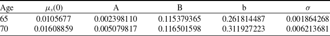
We calibrate the HW model on projected mortality data for each cohort using the least square estimation. The optimal parameters are reported in Table 2:
Table 1. The classical methods’ parameter values.

Table 2. Optimal parameter values for the survival function in the HW model.
It is noteworthy to mention that using a projected for calibration increases the uncertainty, and using observed data would have been more reliable, but as Plat (Reference Plat2009) states: “there is not enough insurance portfolio specific mortality data available to fit stochastic mortality models reliably”.
We have followed the Luciano and Vigna (Reference Luciano and Vigna2015) framework, who have also calibrated the data on UK projected table, and compared between calibrating some stochastic time-continuous models on observed and projected data. They have found that the volatility has lower values in the case of projected data; however, “this seems to indicate that, relying on the observed data, the future evolution of the intensity of mortality for an individual aged x now (observing his/her current force of mortality) presents low variability”.
Zeddouk and Devolder (Reference Zeddouk and Devolder2020a) have followed the same routine using the observed Belgian mortality data and projected data from IA $\rvert$
BE and have found the same conclusions.
$\rvert$
BE and have found the same conclusions.
Therefore, although the data we used is taken from projected mortality tables and not from observed ones, the values of the parameter seem to be realistic and fall within the usual values range. Overall, in practice, if the observed mortality data is available, our framework can be used by a hedger who can directly calibrate the multi-population model to the observed insureds’ mortality data.
Zeddouk and Devolder (Reference Zeddouk and Devolder2019) have computed the prices of the S-forward contracts under the COC and the classical approaches, using HW model for mortality and the assumptions made in this paper. The prices as well as the fixed legs are reported in Table 3:
Table 3. Fixed-legs and S-forward prices under the different methods.

6.1. S-exchange prices in the extra-vol case
We determine the price of the different S-exchange derivatives under the extra-vol effect case using the following parameters:
-
$\tilde{\sigma}=20\%\sigma$
-
$\tilde{\rho}=0.5$
-
$\mu^{\prime}_{x}(0)=\mu_{x}(0)$


The main objective of the paper is to focus on the pricing framework and not really on the calibration itself. Therefore, we have chosen these values for illustration, and a stress test related to each of these values is provided in Section 7. This framework can be used by an insurer who can adjust these values and calibrate the multi-population model to his own mortality data.
Our approach can be even more relevant in case the insurers’ mortality data is weak or not available, but also when this data is available: in this case, the hedger can directly use the insureds’ mortality for calibration and derive the extra volatility by comparing the volatilities of the two population. The correlation can also be easily computed since the data for both population is available.
By studying these parameters, the mortality model will fall in one of the three possibilities we discuss in the paper, and therefore the insurer can observe the volatility effect, trend effect or both (the total effect).
We report in Table 4 the different S-exchange prices computed under the extra-vol effect case:
Table 4. Comparison between S-exchange prices under the different methods, extra-vol case.

6.2. S-exchange prices in the constant shift case
We consider the following parameters:
-
$g=0.9$
-
$\mu^{\prime}_{x}(0)=g\cdot \mu_{x}(0)$


Under this case, we get more or less the same S-exchange prices with the four methods.
6.3. S-exchange prices in the total effect case
We determine the price of the different S-exchange derivatives under the total effect case using the following parameters:
-
$\tilde{\sigma}=20\%\sigma$
-
$\tilde{\rho}=0.5$
-
$g=0.9$
-
$\mu^{\prime}_{x}(0)=g\cdot \mu_{x}(0)$


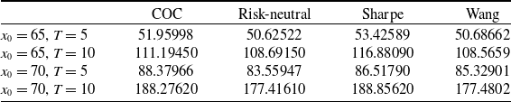
Table 6 represents the different S-exchange prices computed under the total effect case:
Comments:
The S-exchange prices given by Wang and risk-neutral approaches are more or less similar. Overall, the Sharpe method provides the highest S-exchange prices in comparison with the four methods. By comparing Tables 4, 5 and 6, we can also remark that the sum of the prices under the extra-vol and the shift cases is very close to the price found under the total effect case, which results from the cumulative effects of the drift and the volatility.
Also, the price under the shift case is very high when compared to the extra-vol effect, where more than 90% of the price under the total effect is linked to the shift parameter g, and this can be explained by the small values of the volatility $\sigma$
.
$\sigma$
.
7. Sensitivity test
In this section, we perform a sensitivity test for the prices, BEs and RMs computed under the COC approach. For each case, cohort and maturity, we vary one parameter and consider other parameters fixed, and we see how the price of the S-exchange contract under the COC method changes. For illustration, we provide in the Appendix Section the sensitivity test for the classical methods in the total effect case.
Table 5. Comparison between S-exchange prices under the different methods, constant shift case.
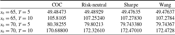
Table 6. Comparison between S-exchange prices under the different methods, total effect case.
7.1. Volatility effect
In this case, to compute the prices of the S-exchange contracts, we have chosen $\tilde{\sigma}=20\%\sigma$
and
$\tilde{\sigma}=20\%\sigma$
and $\tilde{\rho}=0.5$
. Now we use different values of
$\tilde{\rho}=0.5$
. Now we use different values of $\tilde{\sigma}$
and
$\tilde{\sigma}$
and $\tilde{\rho}$
and see how the price changes. The different prices, BE and RM are reported in Tables 7, 8 and 9:
$\tilde{\rho}$
and see how the price changes. The different prices, BE and RM are reported in Tables 7, 8 and 9:
Table 7. Price sensitivity test for $\tilde{\sigma}$
and
$\tilde{\sigma}$
and $\tilde{\rho}$
parameters under COC approach, extra-vol case.
$\tilde{\rho}$
parameters under COC approach, extra-vol case.
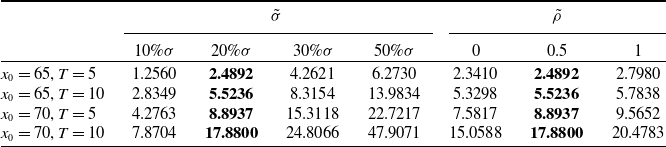
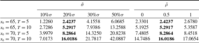
Table 8. Best estimate sensitivity test for $\tilde{\sigma}$
and
$\tilde{\sigma}$
and $\tilde{\rho}$
parameters under COC approach, extra-vol case.
$\tilde{\rho}$
parameters under COC approach, extra-vol case.
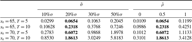
Table 9. Risk margin sensitivity test for $\tilde{\sigma}$
and
$\tilde{\sigma}$
and $\tilde{\rho}$
parameters under COC approach, extra-vol case.
$\tilde{\rho}$
parameters under COC approach, extra-vol case.
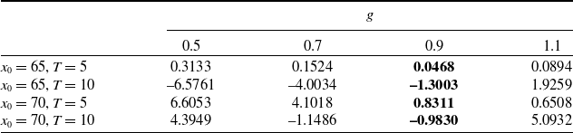
7.2. Trend effect
In this case, to compute the prices of the S-exchange contracts we have chosen $g=0.9$
. We consider now different values for g and see how the price changes. The results are reported in Tables 10, 11 and 12:
$g=0.9$
. We consider now different values for g and see how the price changes. The results are reported in Tables 10, 11 and 12:
Table 10. Price sensitivity test for g parameter under COC approach, constant shift case.

Table 11. Best estimate sensitivity test for g parameter under COC approach, constant shift case.

Table 12. Risk margin sensitivity test for g parameter under COC approach, constant shift case.
7.3. Total effect
In this case, to compute the prices of the S-exchange contracts, we have chosen $g=0.9$
,
$g=0.9$
, $\tilde{\sigma}=20\%\sigma$
and
$\tilde{\sigma}=20\%\sigma$
and $\tilde{\rho}=0.5$
. Let us now compute the price using different values of g,
$\tilde{\rho}=0.5$
. Let us now compute the price using different values of g, $\tilde{\sigma}$
and
$\tilde{\sigma}$
and $\tilde{\rho}$
, then we see how the price changes. The results are reported in Tables 13, 14, 15:
$\tilde{\rho}$
, then we see how the price changes. The results are reported in Tables 13, 14, 15:
Table 13. Price sensitivity test for g, $\tilde{\sigma}$
and
$\tilde{\sigma}$
and $\tilde{\rho}$
parameters under COC approach, total effect case.
$\tilde{\rho}$
parameters under COC approach, total effect case.
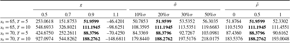
Table 14. Best estimate sensitivity test for g, $\tilde{\sigma}$
and
$\tilde{\sigma}$
and $\tilde{\rho}$
parameters under COC approach, total effect case.
$\tilde{\rho}$
parameters under COC approach, total effect case.

Table 15. Risk margin sensitivity test for g, $\tilde{\sigma}$
and
$\tilde{\sigma}$
and $\tilde{\rho}$
parameters under COC approach, total effect case.
$\tilde{\rho}$
parameters under COC approach, total effect case.

In general, the two populations may have different speeds of reversion: the insurer’s population tends to be wealthier, which would imply a possibly slower mean reversion. The effect of this difference can be measured by analysing the sensitivity of the price with respect to the mean reversion rate parameter. As we mentioned previously, in order to fulfil the independence assumption, the mean reversion rate b in the population’s force of mortality formula should be the same as in the insurer’s population formula. Namely, we should have $b=b^{\prime}$
.
$b=b^{\prime}$
.
In the Appendix Section, we ignore this assumption and perform a sensitivity test on parameter b ′.
8. Different longevity hedging strategies
In this section, we define and compare different longevity hedging strategies using the COC approach. For each strategy, we determine the solvency capital required that the insurer should hold to cover unexpected losses, as well as the BE at time 0.
Depending on his risk aversion, the insurer can choose to hold an SCR and/or to totally or partially hedge the longevity risk. More precisely, we compare the following possible strategies:
-
1. The insurer can choose to hold an SCR and not resort to the financial market or reinsurance to hedge the longevity risk.
-
2. He can choose to only hedge a portion of the systemic longevity risk by entering an S-forward and hold the SCR corresponding to the basis risk.
-
3. In addition to the purchase of an S-forward, he can choose a total protection against the longevity risk by entering an S-exchange contract (assuming that such product is available in the financial market, or proposed by an investor).
-
4. The insurer can choose a total protection without entering an S-forward and an S-exchange, but simply by transferring the total longevity risk to a reinsurer who accepts to take it. The cost of this protection is also assumed to be computed using the COC approach.
-
Auto-protection: holding an SCR (S1)
In this strategy, the insurer manages himself the longevity risk by holding successive annual solvency capitals following the directives of Solvency II. We denote by $_{_{T}}\hat{p}_{_{x}}$
a fixed survival rate of an individual aged x at time 0 to be alive at age
$_{_{T}}\hat{p}_{_{x}}$
a fixed survival rate of an individual aged x at time 0 to be alive at age $x+T$
(
$x+T$
( $\mathcal{F}{}_{0}$
measurable). The premium paid by the insured is based on this fixed rate.
$\mathcal{F}{}_{0}$
measurable). The premium paid by the insured is based on this fixed rate.
The BE in this case is given at time 0 by
 \begin{equation}BE_{0}^{\mathbb{P}}=P(0,T)(E_{\mathbb{P}}\!\left(I(x,T)^{ins}-{}_{_{T}}\hat{p}_{_{x}}\right).\end{equation}
The expression of the successive solvency capitals under the COC approach is given by Zeddouk and Devolder (Reference Zeddouk and Devolder2019):
 \begin{equation}SCR_{i}=VaR_{99,5\%}\!\left[BE_{i+1}^{\mathbb{P}}P(i,i+1)-BE_{i}^{\mathbb{P}}\right],\end{equation}
where
 \begin{align}\nonumber BE_{i+1}^{\mathbb{P}}&=\left(I^{^{ins}}(x,i+1)E_{\mathbb{P}}\!\left(I^{^{ins}}(x+i+1,T-i-1)-{}_{_{T}}\hat{p}_{_{x}}\right)\right)P(i+1,T)\\BE_{i}^{\mathbb{P}}&=\left(I^{^{ins}}(x,i)E_{\mathbb{P}}\!\left(I^{^{ins}}(x+i,T-i)-{}_{_{T}}\hat{p}_{_{x}}\right)\right)P(i,T).\end{align}
Therefore, the estimation of $SCR_{i}\mid_{0}$
can be given by
$SCR_{i}\mid_{0}$
can be given by
 \begin{align}\nonumber SCR_{i}\mid_{0}&=P(i,T)E_{\mathbb{P}}\!\left(I^{^{ins}}(x,i)\right)\left[VaR_{99,5\%}\left(I^{^{ins}}(x+i,1)\right)-E_{\mathbb{P}}\!\left(I^{^{ins}}(x+i,1)\right)\right]\\&\times E_{\mathbb{P}}\!\left(I^{^{ins}}\left(x+i+1,T-i-1\right)\right),\end{align}
and the hedging cost in this strategy is equal to 0.
-
Partial hedging: S-forward (S2)
The insurer choose to partially hedge the longevity risk (its systemic part), by entering an S-forward. In this case, he should pay the price of the S-forward (formula (4.17)) and hold the SCR to cover the eventual losses related to the basis risk. The BE at time 0 is given by formula (4.18), and the estimation of the SCR $_{i}$
at time 0 is given by formula (4.26).
$_{i}$
at time 0 is given by formula (4.26).
-
Total hedging: S-forward + S-exchange (S3)
In this strategy, the insurer prefers not to hold the SCR and to be totally protected against the longevity risk. The cost of this protection is equal to the sum of the S-forward and S-exchange contracts prices.
-
Reinsurance (S4)
Instead of buying an S-forward and an S-exchange, the insurer can directly resort to a reinsurer who accepts to totally cover the longevity risk. In this case, the SCR is equal to 0. For example, if the reinsurer uses the COC approach to compute the price of the total protection, the price of this protection should be equal to:
 \begin{align}\nonumber V_{_{COC}}(0,T)&=P(0,T)\,\left(E_{\mathbb{P}}\!\left[I^{ins}(x,T)-{}_{T}\hat{p}_{x}\right]\right)\\\nonumber &\quad +6\%\sum_{i=0}^{T-1}\big[E_{\mathbb{P}}(I^{ins}(x,i))\left[VaR_{99,5\%}(I^{ins}(x+i,1))-E_{\mathbb{P}}(I^{ins}(x+i,1))\right]\\&\quad \times E_{\mathbb{P}}(I^{ins}(x+i+1,T-i-1))P(0,i+1)P(i,T).\end{align}
For illustration, we compute the different hedging strategies in this section to compare the various strategies that reflect the risk aversion of the insurer.
We use the same data considered in the numerical illustration part of Section 6. We restrict ourselves to two initial ages, 65 and 70 years old, for a maturity of $T=5$
years. Table 16 reports a comparison between the hedging strategies under the COC approach:
$T=5$
years. Table 16 reports a comparison between the hedging strategies under the COC approach:
-
In case S1, the insurer does not buy any protection, but must hold the SCRs corresponding to the longevity risk (the systemic and basis risks). This strategy cost the insurer the expense of holding these SCRs (6% of the SCRs), and the SCRs can be totally or partially lost if things go wrong. In this strategy, however, the insurer is not exposed to credit risk.
-
In case S2, the insurer enters into an S-forward contract, which is an exchange-traded derivative based on the reference population index that partially covers the insurer (systemic risk). Therefore, this insurer should hold smaller SCRs (which can also be totally or partially lost) corresponding to the remaining basis risk. In this strategy, the insurer is exposed to credit risk, but it is limited since the risk is spread among a large number of investors.
-
In case S3, the insurer buys two protections: an S-forward contract from the financial markets and an S-exchange derivative, which is a customised contract OTC. Hence, the insurer will be fully covered against the longevity risk and will not need to set aside an SCR. The credit risk is more significant in this case since it is related to the financial market (S-forward) and the S-exchange’s seller.
-
In case S4, the insurer delegates the risk to a reinsurer, and as in case S3, there is no need to hold SCRs. The cost of this protection is also computed using the COC approach. This strategy represents the highest credit risk since it is related to one entity.
Besides S1, all other strategies the insurer might choose do not completely mitigate the risk, as credit risk must be considered in the risk transfer decision. Credit risk represents a state in which the counterparty (in our case, the financial market or the reinsurer) is unable to fulfil its financial obligations in a timely manner or at all. Neither the financial market nor the reinsurer is completely free from default risk, and therefore, the insurer must hold a capital for this extra credit risk. However, the level of this risk is more important for the reinsurer than for the financial market. Assessment of this risk is beyond the scope of this paper; we refer the interested reader to Biffis et al. (Reference Biffis, Blake, Pitotti and Sun2016) for more details.
Table 16. Comparing different longevity hedging strategies using the COC approach.

The choice of the best hedging strategy depends on the insurer’s risk aversion. Moreover, deciphering the best strategy in terms of cost is difficult at time 0: if the insurer chooses S1 or S2, the cost of the hedging strategy will be known only at maturity of the contract, since it depends on whether or not the SCRs are used to cover the risk. For example, S1 would be better than S3 if the SCRs are not needed; otherwise, S1 would be more expensive than S3 and S4. Additionally, from S1 to S3, the expectation of the cost ( $BE_{0}^{\mathbb{P}}$
+ Price) increases since the expense increases the more the insurer seeks protection against the longevity risk.
$BE_{0}^{\mathbb{P}}$
+ Price) increases since the expense increases the more the insurer seeks protection against the longevity risk.
9. Conclusion
In this paper, we developed a continuous time framework to assess the basis risk through the pricing of a longevity derivative. We proposed a bi-dimensional HW process that can capture mortality trends in the reference population and in the insurer’s population, whose risk is to be hedged. We associated the basis risk with a longevity derivative called S-exchange that we priced under the COC method, which is consistent with Solvency II. We presented this approach as a new benchmark and compared it with other classical pricing methods. In addition, we proposed various hedging strategies depending on the insurer’s risk aversion. For further research, we could price nonlinear longevity derivatives, such as longevity options, using the same cost of capital philosophy.


