


1. Introduction
This paper presents a theoretical analysis of the deformation and stress fields at the junction of two glacier streams. The only previous attempt at such an analysis is that of Reference SharpSharp (1948), who however based his arguments on the erroneous “extrusion flow” hypothesis. There have, however, been a large number of isolated field measurements of surface velocities, strain-rates etc. in confluence zones on a number of glaciers, and recently a very comprehensive study of a confluence on the Kaskawulsh Glacier, Yukon Territory, Canada has been made by Anderton (unpublished).
Any analysis of the deformation at an actual confluence would be most complicated due to the complex irregular geometry of the valley walls. Consequently to make any progress it is necessary to idealize the geometry of the situation quite appreciably. Further, as will be seen below, to make the problem tractable it is necessary to approximate the mechanical behaviour of ice by that of a rigid/perfectly-plastic material. Thus, one cannot hope to obtain any detailed quantitative agreement between such an idealized mathematical model and a specific set of field data. Instead attention is concentrated on investigating the qualitative features of the deformation and stress fields and their dependence on the defining parameters. It is hoped that the results presented here will form a basis for discussing the morphology of confluences such as crevasse and foliation patterns.
The valley walls will be assumed to be parallel and vertical and the deformation is assumed to be in plane strain, so that the deformation pattern is independent of the depth below the surface. In view of these restrictions the “inset” and “overlaid” conditions (Reference SharpSharp, 1948) fall outside the scope of this theory. Some indication of the way in which this simple two-dimensional picture must be modified to meet the actual three-dimensional situation will come out in the analysis. It is shown that the flow planes which here are assumed to be parallel to a flat inclined bed will in fact, become twisted at a confluence due to a secondary flow (Fig. 23).
The mechanical model which best fits the experimental data on ice is the power-law creep relation between stress and strain-rate (Glen's law). Boundary-value problems involving these creep equations are extremely complex and difficult to solve in two- or three-dimensional situations. Consequently, with one exception (Reference NyeNye, 1957), all glacier flow theories using these equations are one-dimensional. However, one can make progress with two-dimensional problems if one lets the exponent in Glen's law n (≈ 3 or 4) tend to infinity. In the limit Glen's equations go over to those for a rigid/perfectly-plastic material with a Mises yield criterion (Reference NyeNye, 1953). Such a material behaves rigidly as long as τ < k where τ is the “effective shear stress” and k is a material constant. When τ = k the material deforms al an indefinite rate but in such a way that the components of the strain-rate and stress-deviator tensors are proportional. The condition τ > k cannot occur. This approximation was first used by Reference NyeNye (1951) when he modelled a glacier by a two-dimensional block of rigid/perfectly plastic material resting on an inclined plane. More recently the same approximation has been employed in an analysis of a glacier snout (Reference NyeNye, 1967) and of the erosion of irregularities on a glacier bed (Reference Nye and MartinNye and Martin, 1968).
Above and below the confluence zone the ice is assumed to move rigidly as in “plug flow”. This is a particularly good approximation in the equilibrium-line region where the longitudinal strain-rates are small. The deformation is hence localized to a definite zone. Mathematically this is a consequence of the hyperbolic nature of the governing equations for rigid/perfectly-plastic materials under plane strain conditions. The corresponding creep equations are elliptic (Reference BergBerg, 1967), so that in a creep model the deformation caused by the merging of two ice streams would not be confined to a specific zone but would extend an indefinite distance up each arm of the glacier. The presence of a definite deformation zone in the plastic model is a distinct theoretical advantage, making the problem much more readily tractable.
The actual deformation in this zone will take two forms:
-
(a) discontinuities in tangential velocity across certain curves (slip lines), which on a real glacier correspond to narrow bands of intense shear. Such bands are frequently observed in the confluence zones of temperate glaciers and show up particularly well in air photographs where they may be seen to cause kinks in longitudinal structures and moraines.
-
(b) regions of continuous deformation in which the strain-rates are finite.
One of the prime objectives of this investigation is to find the number, position and strength of these velocity discontinuities (shear bands). As will be seen these factors depend critically on the overall geometry of the junction and on the relative velocities of the two converging streams.
To complete the posing of the problem, it is necessary to specify some boundary conditions on the valley walls. The normal component of velocity must, of course, be zero. The other required condition is some frictional law on the tractions. There would still appear to be some considerable doubt about what this law should be. The approach adopted here is to produce solutions for two extreme conditions, perfectly lubricated (no shear stress) and perfectly rough walls (shear stress = k, the yield stress), and to compare and contrast the corresponding deformation patterns. Most surface strain-rate measurements such as those reported by Reference MeierMeier (1960) from the Saskatchewan Glacier and by Anderton (unpublished), would indicate that the valley wall is close to being a maximum shear stress trajectory so that the latter is probably the more correct assumption. This is indeed the condition employed by Reference NyeNye (1967) and Reference Nye and MartinNye and Martin (1968) with reference to the bed of the glacier. As will be seen, however, several of the solutions are the same under both frictional conditions.
The basic properties of solutions to plane-strain rigid/perfectly-plastic problems are reviewed in the next section in terms of slip-line fields and the hodograph diagram. In section 3 solutions are presented for configurations in which a tributary enters at the side of a main stream. Several types of solutions are required to cover the range of all possible geometric and kinematic conditions. The specific form of solution valid for a particular confluence can be read off from one of two nomographs. The possibility of interference between the two deformation zones when two tributaries enter a main stream in close proximity is examined in section 4, whilst solutions for the confluence of two main streams (Y-junction) is considered in the final section. In addition the field data obtained by Anderton on the Kaskawulsh Glacier are compared with a theoretical solution.
2. Slip-line fields and the hodograph diagram
The state of stress in a plane-strain deformation of a rigid/perfectly-plastic material is most conveniently discussed in terms of “slip-line fields”. For a full account of the theory the reader is referred to one of the standard texts such as Reference HillHill (1950), Reference Prager and HodgePrager and Hodge (1951), Reference PragerPrager (1959); Reference Johnson and MellorJohnson and Mellor (1962) or Reference Ford and AlexanderFord and Alexander (1963). Slip-lines are the trajectories of maximum shear stress (and also maximum shear strain-rate) and consist of two families of mutually orthogonal curves. The two families are labelled α- or β-curves, chosen so that the maximum principal stress lies in the first and third quadrant of the (α, β) coordinate system (we adopt the convention used in metal plasticity of regarding tensile stresses as positive). Since the directions in which the shear stress is a maximum make angles of 45° with the principal directions, it follows that the principal directions at any point bisect the slip-line directions.
The state of stress acting on an elemental curvilinear rectangle whose sides are parallel to the slip-lines at a typical point in the plastic zone is shown in Figure 1. The stress consists of a shear stress k, the yield stress of the material, and an all-round hydrostatic pressure p. Once the value of p has been obtained at one point in the network of slip-lines it can be deduced at any other point by using Hencky's relations:
ɸ being the anticlockwise inclination of the α-line to some fixed reference direction. The characterizing properly of slip-line nets which distinguish them from any other set of orthogonal curves is embodied in Hencky's Theorem. This states that “the angle between two slip-lines of one family, where they are cut by a slip-line of the other family, is constant along their length” as illustrated in Figure 2. A system of curves having this property is frequently referred to as a “Hencky–Prandtl net”.

Fig. 1. Stress system at a typical point in a slip-line field.

Fig. 2. The Hencky–Prandtl property of slip-line fields.
Corresponding to Equations (1) are relations which state how the velocities vary along the slip-lines. If (u, v) are the components of velocity along the α- and β-lines respectively, then
These are Geiringer's equations and can be given a most useful geometric interpretation in the velocity or “hodograph” plane. (For full details see Reference GreenGreen (1954), Reference PragerPrager (1953) or the last three texts cited above). Referring to Figure 3, we represent the velocity at a typical point p in the slip-line field by a vector OP in the velocity plane. As p traces out an α- or β-slip-line in the physical plane its image p traces out an α’ or β’-curvc in the velocity plane. It is shown in the above references that Equations (2) imply that this image curve is everywhere orthogonal to the original slip-line. Thus, in Figure 3, the tangent to the α'-curve at p is perpendicular to the tangent to the α-curve at P and is, therefore, parallel to the tangent to the β-curve at P. It follows also that the complete net of curves in the hodograph plane possess the characteristic Hencky-Prandtl property described above.

Fig. 3. Representation of velocity vector in (a) physical plane, (b) velocity or hodograph plane.
It is important to note that there can be two image curves in the hodograph plane to one slip-line. This occurs when the tangential velocity is discontinuous across a slip-line. Such a discontinuity, however, must be constant in magnitude, the two sides of the slip-line hence map into two parallel curves. It frequently happens that the material on one side of a discontinuity translates rigidly. The image of such a rigid region in the velocity plane is just a single point, and so the image of the plastic side of the dividing slip-line is a circular are centred on this point. This construction will frequently be needed in the following.
3. Single tributary
(i) Statement of problem
In this section we consider the problem of a tributary entering a main-stream (Fig. 4). To cut down the number of independent parameters we shall assume that the width of the main stream is the same above and below the confluence. The geometry will hence be completely specified, apart from scale, if we know the ratio of the main-stream width to that of the tributary entrance (d/h) and the angle δ between the converging channels. If we also know the ratio of velocities in these two channels (U1/U2 ) then, as will be shown, the deformation is determined provided we assume that the ice in the lower channel moves as a single rigid mass.
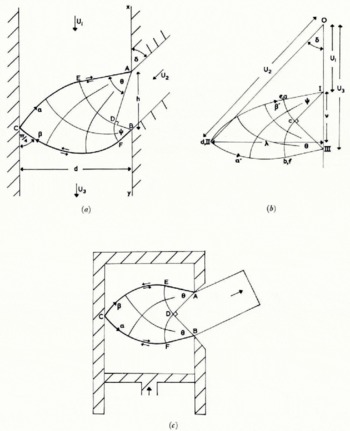
Fig. 4. Basic solution for single tributary with smooth walls (a) slip-line field, (b) hodograph. (c) slip-line field for sideways extrusion.
It has been suggested that the two ice streams might flow independently in the lower channel with different velocities. There would, therefore, be a velocity discontinuity (shear band) along the dividing stream-tine. However, measurements reported by Reference MeierMeier (1960), Anderton (unpublished) and Reference Allen, Allen, Kamb, Meier and SharpAllen and others (1960) indicate that although there may be intense shear in the region of the bounding stream-line immediately below the junction, this is not present further down-stream (distance of order ½h say). This is indeed what one might expect. Near the junction the dividing stream-line is very nearly in the direction of the maximum shear stress and hence if the dirty ice/ice interface shears more easily than the bulk of the ice, it may well do so here. Further down-stream, however, the dividing stream-line is much closer to the direction of principal stress and, therefore, not subject to any appreciable shear. In the analysis presented here the mechanical properties of the interface between the two streams are assumed to be identical with those of any other surface within the bulk of the ice. As will be seen, this theory predicts that a velocity discontinuity (shear band) will occur close to, but not coincident with, the bounding streamline just below the junction. Thus it is not clear whether the intense shear reported by Meier, Anderton, and Allen and others is due to shearing in the bulk of the ice or to slipping along the dividing stream-line.
The velocities Ul and U2 of the two impinging streams depend essentially on the sizes of the two accumulation basins up-stream of the confluence. These, of course, can be very different and hence the ratio Ul/U2 can differ significantly from unity. It will be shown that the value of this ratio is critical in determining the nature of the deformation pattern at the confluence.
The problem is hence completely specified by the three parameters d/h, δ and Ul/U2 . The velocity U3 in the lower channel is determined in terms of Ul or U2 by the mass conservation condition:
If we reverse the direction of the velocities this problem is seen to be very similar to the sideways plane-strain extrusion process (Fig. 4(c)). The solution to this, and many similar extrusion problems, may be found in the monograph by Reference Johnson and KudoJohnson and Kudo (1962). There is, however, one important difference between the glacier confluence problem and the extrusion problem, which makes the former rather more difficult to solve. In the extrusion process the extruded billet, corresponding to the tributary, is not constrained to move in any particular direction, instead its direction is determined by the condition that it is free of any lateral force. In our problem, however, δ is specified and in general there will be a lateral pressure (to be determined), exerted by one of the valley walls on the ice stream.
(ii) Basic solution for smooth walls
The form of the slip-line solution for this problem, assuming the valley walls are perfectly smooth, is shown in Figure 4(a) and the hodograph in Figure 4(b). The slip-line field consists of two “centred fan” regions ADE and EDF in which the slip-lines of one family are straight radial lines and of the other are circular arcs. The remainder of the field DECF is defined uniquely as the field between the two circular arcs DE and DF. In Reference HillHill's (1950) nomenclature this is an example of a boundary-value problem of the first type. The hodograph net is rather similar and consists of two centred fans Ica and IIIcb of equal radii and the field defined by the two equal circular arcs ca and cb. This particular field occurs frequently in solutions to boundary value problems and may be found tabulated in Reference HillHill (1950) or Reference EwingEwing (1967). The vectors 01 and 0111 represent the velocities U1 and U3 of the main stream above and below the confluence, and 0II represents the velocity U2 of the tributary. Here, as elsewhere in this paper, we shall adopt the standard convention of denoting the images in the velocity plane of points in the physical plane by the appropriate lower case letter. The two centred fans in the hodograph represent the velocity discontinuity, of magnitude (U3 — U1)/√2, along AECFB. Slip-lines across which the velocity is discontinuous are shown as heavy lines and the direction of the tangential discontinuity indicated by small arrows (cf. AEC and CFB in Figure 4(a)).
The corresponding extrusion slip-line field (Fig. 4(c)) is a particular case of the above solution, valid when the radii of the two centred fans are equal.
The solution of Figures 4(a) and (b) is completely determined by the two vertex angles of the centred fans θ and Ψ, and hence has two degrees of freedom. At first sight this solution appears not to be determinate since, as discussed above, three parameters are needed to set up the problem. This paradox is resolved by noting that the slip-line field depends only on the relative velocity of the two converging streams, and hence only on a certain combination of the parameters U1/U2 and δ and not on each separately. Thus, the field depends only on the position of 11 relative to 1, in the hodograph diagram, and not on its position relative to the origin. This can best be seen by considering the effect of superimposing a constant velocity V in the main-stream direction. This, of course, has the effect of changing the inflow angle δ. U1 U3 and the component of U2 in the main-stream direction are all increased by the same amount V, whilst the component of the tributary velocity perpendicular to the main stream [U2 sin δ) is unaltered. The mass conservation condition, Equation (3), is hence automatically satisfied, and the original slip-line field is also the solution to this new problem. In the hodograph diagram the effect of superimposing this extra velocity is to move the origin up or down the I-III axis, but to leave the actual hodograph net unaltered.
For convenience we take the length of I III, (U3-U1 ), as the unit of length in the hodograph plane. The position of II, relative to I, is hence completely specified by the dimensionless cartesian co-ordinates (v, λ) as shown in Figure 4(b), and defined by
The last equality in (5) follows from the mass conservation condition (3). Eliminating U3 from Equation (3) we can also express v only in terms of the three defining parameters d/h, U1/U2 and δ:
λ is a purely geometric factor depending only on the geometry of the junction but v depends also on the relative velocity of the two converging streams.
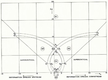
The procedure for constructing the solution is as follows. Evaluate the parameters λ and v from Equation (5) and (6) for the particular confluence in question. Use the hodograph diagram, which as stated above is a well tabulated net, to evaluate the two angles θ and ψ. (The boundary of this net is, in fact, shown in Figure 5, it being the part marked SA.) Once we know these two angles we can construct the slip-line field using any one of the standard techniques such as the grid method (Reference HillHill, 1950), the graphical procedure (Reference PragerPrager, 1959) or the series method (Reference EwingEwing, 1967). (This particular field can also conveniently be constructed by a transformation technique described by Reference CollinsCollins (1968[a], section 8).)
The hodograph net is symmetric about the line v = ½ (Figs. 4(b) and 5). When v = ½, θ = ψ and U2 cos δ = ½ (U1+U3 ) which is the extrusion situation. As v gets greater or less than ½, U2 cos δ is greater or less than ½ (U1+U3 ) from (4), θ is greater or less than ψ and the deformation tends to be displaced down- or up-stream in the sense that c (Fig. 4(a)) lies below or above the mid-point of AB. If the tributary enters at right angles to the main stream, so that δ = 90°, (a T-junciion) the deformation zone will always tend to be displaced up-stream since U2 cos δ = 0 < ½ (U1+U3 ).
A particular example of this field has been computed, but before discussing this we consider some other types of solution. The one considered above can be regarded as the basic solution, but it will not cover the complete range of configurations that can arise. In other words, it is not always possible to find a solution of this type corresponding to every possible combination of λ and v.
(iii) Other solutions for smooth walls
The above solution can break down in three ways. Consider the effect of keeping the geometric factor λ fixed and varying v. As v increases (or decreases) from ½ the slip-line field becomes more and more asymmetrical until either |θ — ψ| = ¼π or one or other of θ and ψ becomes a right angle. As can be seen from Figure 5, the former occurs if 0.5 ≤ λ ≤ 2.5 and the latter if 2.5 ≤ λ ≤ 6.2.
In the first situation, the slip-line field is as shown in Figure 6(a) or 6(b); in both cases there is a straight slip-line across the entrance AB to the tributary. The critical values of (λ, v) for which this occurs lie on the curves PQ 0, Q 0 in Figure 5. For values of v beyond these critical values the slip-line field is exactly the same as for the critical case (i.e. as in Fig. 6(a) or 6(b)), but an additional velocity discontinuity must be put across the slip-line AE at the mouth of the tributary. Typical hodographs for these supercritical solutions are shown in Figures 6(c) and 6(d).

Fig. 6. Supercritical solutions for smooth walls and 0.5 ≤ λ ≤ 2.5. (a) slip-line field v > ½, (b) slip-line field v ½, (c) hodograph v > ½, (d) hodograph v < ½.
In the second situation when θ (or ψ) = ½π, we cannot continue with the basic type of solution since the angle EÂX (or FBY) in Figure 4(a) would be less than (¼π and the material in this vertex, which we postulate to be rigid, would, in fact, deform plastically (this is an example of a general result due to Reference HillHill, 1954). Instead we must go over to another type of solution in which the material is plastic along part of the inner main-stream wall. Such a solution (applicable when v < ½) is shown in Figure 7. The domains of validity of this type of solution in the (v, λ) plane are marked SB (v > ½) and SB' (v < ½) in Figure 5. This diagram is, in fact, just the hodograph of this new solution, which turns out to be simply an extension of the hodograph for the basic solution. This extended hodograph (Fig. 5) is hence a highly convenient nomograph since for given λ and v it enables one to read off the form of the appropriate solution, and also if plotted to a large enough scale, the angles of the relevant centred fans.
The deformation pattern differs from that previously considered in that it spreads up (down)-stream along the inner wall according as v is less(greater) than ½, and in that two velocity discontinuities (shear bands) emanate from B(A) both with magnitude (U3—U1 )/√2. Just as for the basic one this solution breaks down when the tributary entrance AB becomes a slip-line. This happens on the curves Q 1s1 and Q 1s1' in Figure 5. For values of |v| greater than these critical values the solution is again formed from the critical solution by adding a velocity discontinuity along the slip-line AB.

Fig. 7. Slip-line field valid in region SB' in Figure 5. The corresponding field valid in SB is similar except that the deformation spreads down-stream along the inner main-stream wall and not up-stream.
These solutions do not apply if the (v, λ) point lies above R1S1 or R1'S1' in Figure 5, in which case the deformation spreads both up- and down-stream along the inner wall of the main channel. The slip-line field is not illustrated but is a natural extension to that of Figure 7. Its domain of validity is marked SC in Figure 5.
The solutions valid in the small intermediate regions between the parallel curves Q0R0R1'S1', Q1R1R2S2 ’and Q’0R0R1S1 , Q1’R1’R2S2 in Figure 5 have been found in principle but are not discussed here. They are of a very much more complicated type similar to that discussed by Reference GreenGreen (1962) and Reference CollinsCollins (1968[b]) for extrusion.
Finally, the solution corresponding to region SD in Figure 5 is shown in Figure 8. This corresponds to values of λ = d/h rather smaller than is met with in practice and will not be discussed in detail except to note that the magnitudes of the velocity discontinuities in this solution are rather less than (U3—U1 )/√2.

Fig. 8. (a) Slip-line field, (b) hodograph of solution valid in region SD in Figure 5.
It should also be noted that any of the above solutions will break down, due to over-stressing of the proposed rigid regions, if the angle between the bounding slip-line and the tributary wall is less than ¼π. This can never happen, however, if δ lies in the range ¼π ≤ δ ≤¾π.
(iv) Right-angle junction with smooth walls
The effect of varying any of the defining parameters on the deformation can be deduced from the nomograph (Fig. 5). To be specific suppose we take δ = ½π (a T-junction) and consider the effect of varying the geometric factor λ = d/h and the velocity ratio U1/U2 (= —v/λ when δ = ½π). The zones of validity of the three basic types of solution can be shown in a (d/h, U1/U2 ) diagram as in Figure 9(a). As already noted the deformation zone will always be displaced up-stream. The values of (U1/U2 ) at which the solutions become supercritical and velocity discontinuities appear across the tributary mouth is seen to be approximately unity for d/h > 4, but is rather less than unity for d/h < 4.

Fig. 9. Nomograph for right-angle junction (T-junction) for (a) smooth walls, (b) rough walls.
(v) Solutions for perfectly rough walls
The basic solution for perfectly rough walls is shown in Figure 10. It differs from that for smooth walls in that the bounding slip-lines meet the far wall tangentially and at right angles instead of at 45°. Also there is now only one velocity discontinuity (shear band), which emanates from the upper junction corner. Its magnitude is (U3 — U1 ) and is hence √2 times stronger than the corresponding discontinuity in the smooth-wall solution. Just as before, the angles θ and Ψ must be chosen so that λ and v take the prescribed values, and again, just as before, we can use the hodograph diagram as a nomograph for this purpose. This is shown in Figure 11, the zone of validity of the present solution being RA. This field is in fact part of the singular Hencky–Prandtl net constructed on the convex side of the circular are III NM. Unlike Figure 5, the corresponding diagram for smooth walls, this nomograph is asymmetrical about v = ½. In addition the deformation zone will always tend to be displaced down-stream of the midpoint of AB.

Fig. 10. Basic solution for single tributary with rough walls (a) slip-line field, (b) hodograph.
The basic solution will break down when ψ — θ = 0 or ½π, for in either case the tributary mouth AB has become a slip-line. This happens on the curves m p and NQ respectively in Figure 11. For values of v outside these ranges the solution is supercritical and is obtained from the critical solution by adding a velocity discontinuity across the tributary mouth AB.

Fig. 11. Nomograph for single tributary with rough walls. Solutions valid in regions RA, RB and RC are shown in Figures 10, 12(a) and 12(b), respectively.
The basic solution does not now break down, however, when EÂX (or FBY) is less than ¼π, since such a vertex is not over-stressed when the wall is perfectly rough (Reference HillHill, 1954). Instead we have to go over to another type of solution when one or other (or both)of these angles become zero. This occurs when Ψ = π or θ = ½π; in fact, since Ψ — θ ≤ ½π the first condition can only occur if the latter also applies. In other words, the deformation can only spread upstream along the inner wall if it also spreads down-stream along this wall. The form of the slip-line field when the deformation spreads down-stream is shown in Figure 12(a) and when it spreads in both directions in Figure 12(b). The domains of validity of these two solutions are regions RB and RC respectively in the (v, λ) diagram (Fig. 11).

Fig. 12. Slip-line fields of solutions valid in regions (a) RB and (b) RC.
(vi) Rigid-angle junction with rough walls
If we make the same specialization as in (iv) above, i.e. δ = ½π, the domains of validity of the three types of solution can be shown in a (d/h, U1/U2 ) diagram (Fig. 9(b)). The general form of this diagram is similar to that for smooth boundaries, although the basic field (RA) is valid for a rather larger range of values of d/h than the corresponding field for smooth walls (SA). Also the solutions now become critical at a rather lower value of U1/U2 , (≈ 0.7 compared with unity).
(vii) An example
Solutions for a particular example of a right-angled junction are shown in Figure 13. The ratio λ = d/h = 2.5, whilst Ul/U2 = 0.5 so that v = —1.25 from Equation (6). Using either Figure 5 or 9(a) we see that this confluence is critical if we assume the walls are smooth, but Figure 11 or 9(b) indicates that it is supercritical if the walls are rough. In the first case there will be a slip-line but no velocity discontinuity across the tributary entrance, in the second case there will be both. The slip-line field solutions for these two conditions are shown in Figures 13(a) and (b), together with some typical stream-lines. The direction of the streamline through any point is given by the vector from the origin to the image point in the hodograph diagram. Stream-lines are hence very easily plotted graphically using the hodograph diagram (for further details see Reference PragerPrager (1959)).
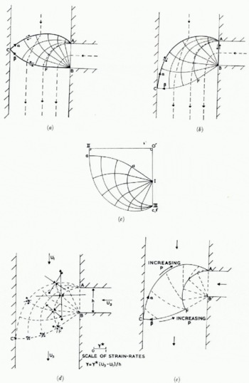
Fig. 13. An example of a T-junction (β = 90°) with λ = d/h = 2.5, U1/U2 = 0.5. (a) slip-line field for smooth walls, (b) slip-line field for rough walls.(c) hodograph for rough walls, (d) principal strain-rates (rough walls), (e) constant pressure contours (rough walls).
The hodograph diagram for the rough-walled case is shown in Figure 13(c), whilst the magnitude and directions of the principal strain-rates at some representative points are shown in Figure 13(d). The magnitude of the principal strain-rates ±γ can be conveniently evaluated from the expression (Reference GreenGreen, 1954)

where R, S, R',S' are the radii of curvature of the α-, β-, α'-, β'-curves respectively. In the centred fan region ABF, γ is inversely proportional to the radial distance from the vertex B, and theoretically infinite actually at this vertex.
Figure 13(e) shows curves (dashed) of constant pressure p through nodal points of 25° angular separation. In order to keep the deformation one of plane strain the compressive stress normal to the flow planes must be equal to p, the all-round hydrostatic pressure (cf. Reference HillHill, 1950, chapter 6). In going from one nodal point to the next in Figure 13(e) this pressure changes by 2k Δα, where Δα = 0.436 which is 25° in radians. This follows from Hencky's relations, Equations (1). Now just such a change in normal stress would occur if the thickness of the ice above the flow plane in question differed by an amount 2h0 Δα (where h0 = k/pg, p being the density, g the acceleration due to gravity) between these two points. Thus, the way in which p varies throughout the deformation zone reflects the variation in surface height throughout the confluence zone. In particular, the constant pressure curves in Figure 13(e) correspond to contours on the glacier surface.
This argument of course assumes that the deformation is, in fact, plane strain. It would be highly fortuitous, however, if the local accumulation/ablation distributions were such that the surface topography as predicted above represented a steady-state situation. Nevertheless, this way of identifying the constant-pressure curves of the slip-line field solution with surface contours at least gives some indication of the overall shape, position and magnitude of the surface disturbance at a confluence. In any case it is not possible to do any better without recourse to a three dimensional analysis.
An alternative method of obtaining a varying normal stress over these planes is to superimpose a secondary flow in each cross-section of the glacier. The type of secondary How envisaged is shown in Figure 23 with reference to the deformation at a Y-junction. As will be described in section 5(iv) there is some field evidence for just such a flow pattern. Due to the non-linearity of the governing equations we cannot, of course, quantitatively superimpose two velocity fields, rather these considerations only indicate qualitatively the possible nature of the actual three-dimensional flow.
The bulges which actually occur at the confluence of two glaciers are typically 20–30 m in height. This value is rather less than is predicted from identifying surface contours with the constant pressure curves of the slip-line solution. For example, if we take k ≈ 1 bar, h0 ≈ 11 m, the maximum change in surface height for the example in Figure 13(e) is ≈ 60 m. This discrepancy would be accounted for by the type of secondary flow described above, since this tends to thin the ice in regions where p is large but to thicken it correspondingly where p is small.
4. Interference between tributaries
In this section we consider the problem of two tributaries entering a main stream, one on each side of the channel. If the entry regions are sufficiently far apart the solution is obtained simply by considering each confluence separately and constructing two separate deformation zones as described in the previous section. However, if the relative separation is small, the two slip-line fields would overlap and there must, therefore, be some interference between the two deformation zones.
The slip-line field and hodograph solutions to this problem are shown in Figure 14. The solution has five degrees of freedom: the angles θ, Ψ, θ', Ψ' and the inclination of the slip-lines at c to the main channel direction. These five angles are to be chosen so that the five defining quantities d/h, d/h’ the relative velocity of the two tributaries to the upper main-stream flow and the eccentricity e (as defined in Figure 14(a)) take specified values. Due to the larger number of variables involved no attempt has been made to construct a nomograph corresponding to Figures 5 and 11 for a single tributary.
The analysis is very much simplified, however, if the confluence is symmetric (δ = δ’, U2/U2’ h = h') with zero eccentricity. In this case the slip-line field is symmetrical about the mid-line of the main-stream. The slip-lines meet this line at C and at an angle of 45°. We need, therefore, only consider one half of the solution and apply the analysis of the previous section for a single tributary but with d replaced by ½d.
It is to be noted that the solution of Figure 14 is valid for both types of frictional condition on the valley walls (smooth or rough) provided none of the postulated rigid vertices has included angle less than 45° (in this case the smooth wall solution must be modified as in the previous section). Figure 14, of course, only shows the “basic solution” and will not cover all possible geometries and velocity conditions. It can, however, be easily extended on the same lines as for the single tributary.

Fig. 14. Basic double tributary solution (e ≤ e1) (a) slip-line field, (b) hodograph.
Consider now the effect of increasing the eccentricity e, whilst keeping the other defining parameters fixed. As e increases the direction of the α-line at C (Fig. 14) approaches the vertical. At this critical point (e = e1 , say) the magnitude of the velocity discontinuity on the α-line has increased to (U3 – U1 ) whilst that on the corresponding β-line A'E'CFB has decreased to zero. For e > e 1, the solution cannot be of the type shown in Figure 14 since the velocity discontinuity along the β-line would have to be of the opposite sign and would involve a negative work rate. Instead the solution is as shown in Figure 15. The two deforming regions are exactly the same as when e = e 1 but are now relatively displaced and joined by a single straight slip-line CC, with velocity discontinuity (U3-U1 ) separating two rigid regions.

Fig. 15. Double tributary solution for e1 ≤ e ≤ e2.
In this way we can postulate solutions of this form for all e > e1 . However, we can find solutions, as discussed at the beginning of this section, consisting of two completely separate non-overlapping deforming regions. It would thus appear that we have two completely different possible solutions. This paradox is resolved by appealing to the uniqueness and bound theorems of rigid/plasticity theory (Reference HillHill, 1951). In the present context these enable us to say that the true solution is the one involving the smaller total rate of energy dissipation. The other solution will be invalid because the material in part of the postulated rigid regions will, in fact, deform plastically. Thus the solution in Figure 15 will only be valid for a finite range of eccentricities e1 ≤ e ≤ e2 say and the solution consisting of two unconnected deforming zones is valid for e e2 . The value of the critical eccentricity e2 is obtained by equating the total rates of dissipation in the two solutions.
The evaluation of these two critical eccentricities is extremely complicated in general, and we are here content with obtaining typical values which relate to the corresponding extrusion problem with equal orifices (Reference Duncan, Duncan, Johnson and OvresetDuncan and others, 1966). The extrusion situation is much simplified since Ψ' = θ, θ' = Ψ and the radii of the centred fans in each of the two deforming zones are equal. The critical eccentricities are obtained by using approximate analytical expressions for the extrusion pressures giving e1 ≈ 1 and e2 ≈ 2; these values being (approximately) the same whether the walls are assumed rough or smooth.
5. Confluence of two main streams
(i) Simplest case—two straight velocity discontinuities
Consider now the junction of two main streams as shown in Figure 16. To reduce the number of defining parameters, we will only consider geometries in which the lines across the mouths of the two converging streams are perpendicular to the valley walls, so that CÂX and BÂY in Figure 16 are right angles. The problem is completely posed if we know the ratios d2/dl U2/U1 and the angles δ, and δ2. d3 and U3 are then determined by geometry and mass conservation respectively:
For certain values of these parameters the deformation is particularly simple, consisting of just two velocity discontinuities (shear bands) across the mouths of the two upper streams (Fig. 16(a)). From the corresponding velocity diagram (Fig. 16(b)), we see that this solution is valid only when the velocity ratio is
(ii) Symmetric junction
For more general velocity ratios the situation is rather more complicated and it is convenient first to consider junctions with symmetric geometries (d1 = d2 , δ1 = δ2). The simple solution of Figure 16 is only valid for a symmetric junction if U2/U1 = 1. We now consider the effect of varying this ratio and without loss of generality we may suppose U2/Ul 11.

Fig. 16. Confluence of two main streams (Y-junction). The simplest solution consisting of just two velocity discontinuities (shear bands) AB and AC. (a) slip-line field, (b) hodograph.
A solution to this problem is shown in Figure 17 with the associated hodograph. The slip-line field BAD is a centred fan whilst ADE has a singularity at A and is defined by the circular are AD, CE is a straight velocity discontinuity on either side of which the material moves rigidly.

Fig. 17. Solution for symmetric Y-junction for 1 ≤ U2/U1 ≤ (U2/U1)crit. (a) slip-line field, (b) hodograph, (c) velocity vectors.
For symmetric junctions the conservation of mass condition, Equation (9) reduces to
From this condition it follows by simple trigonometry that the speeds of the two upper streams relative to the lower one (L1 and L2 in Figure 17(c)) are both equal to (U2/3 — U1U2 )½, which is the value of the velocity discontinuity along AEC. It follows from this result and the fact that d1 = d2 that the slip-line and hodograph nets are geometrically similar.
If we produce 11 Q to meet 0 III at T in Figure 17(b), we see that T must lie below III and hence U3 cos δ < U2 . From Equation (11) it follows that U2/U1 is indeed greater than unity. Thus, the straight (and weaker) velocity discontinuity occurs across the mouth of the stream with the greater velocity.
As U2/U1 , increases a critical point is reached at which E and C coincide. Also, since the slip-line field and hodograph are geometrically similar, II and Q also coincide, so that the velocity discontinuity on AB vanishes concurrently with the length CE. For values of U2/U1 greater than this critical value the solution is as shown in Figure 18, it being very similar to the basic solution for a single tributary. There is now no velocity discontinuity across the mouth of the 2-stream, instead that along AEC is reflected back (though with diminished magnitude) along CDB. Again the hodograph (Fig. 18(b)) is similar to the slip-line field.

Fig. 18. Solution for symmetric Y-junction for U2/U1 (U2/U1)crit. (a) slip-line field, (b) hodograph.
These solutions are valid for all frictional conditions provided all rigid vertices are greater than 45°, otherwise the solution for smooth walls must be modified as previously.
The values at which (U2/U1 ) becomes critical and the solution goes over from that of Figure 17 to that of Figure 18 is shown plotted against δ in Figure 19. As δ increases from zero, (U2/U1 )crit increases from unity and tends to infinity as δ → 60°. At this angle Ψ = 0 and C and D coincide (Fig. 17(a)) and for δ > 60° the solution is always of the type shown in Figure 17.

Fig. 19. Plot of (U2/U1)crit. against δ for symmetric Y-junction.
(iii) Asymmetrical junction
We now consider the more general situation of an asymmetrical junction (δ1 ≠ δ2, d1 ≠ d2 ). The basic solution is shown in Figure 20 and is valid for a range of values of U2/Ul cos δ2/cos δ1. This solution differs from the corresponding solution for a symmetric junction (Fig. 17) as in general the slip-line field and hodograph are not now totally similar in that the lengths EC and Q II are not proportional. From the general mass conservation condition (9) it is easy to show that the speeds of the two upper streams relative to the lower stream (L1 and L2 , in Figure 20(c)) are related by
so that
Thus the slip-line and hodograph diagrams are completely similar if and only if d1 sin δ1 = d2 sin δ2; i.e. if BC is perpendicular to the walls of the lower channel.

Fig. 20. Solution for asymmetric Y-junction for cos β2/cos β1 ≤ U2/U1 ≤ (U2/ U1)crit. (a) slip-line field, (b)hodograph, (c) velocity vectors.
Consider now the effect of increasing U2/U1 , until the solution breaks down for some reason: we distinguish three cases depending on the relative positions of A, B, and c.
-
a. If BC is perpendicular to the lower channel walls, CE (Fig. 20(a)) and Q 11 (Fig. 20(b)), the velocity discontinuity on AB, vanish together as in the symmetric case since the slip-line and hodograph diagrams are totally similar. For larger values of U2/U1 we go over to a solution of the type shown in Figure 18 for a symmetric junction.
-
b. If C lies below B, then L1/d2 > L2/d1 , from Inequality (13) and hence Q II vanishes before CE does. In this case we must go over to a field of the type shown in Figure 21(a), where AEC is still a velocity discontinuity but AB is no longer a slip-line. This field remains valid until CE also vanishes and we then switch to the solution in Figure 18 as in (a) above.
-
c. If C lies below B, then Ll/d2 < L2/d1 , and this time the length CE vanishes first. When this happens the solution goes over to that shown in Figure 21(b), which involves three velocity discontinuities. We again go over to the Figure 18 solution when U2/U1 , has increased to the point where Q II also vanishes.

Fig. 21. Intermediate slip-line field solutions for asymmetric Y-junction, (U2/U1) > (U2/ U1)crit. (a) c below B, (b) B below c.
In principle we can, therefore, construct solutions to cover all possible velocity ratios. However, no attempt has been made to compute the various critical velocity ratios for the general asymmetrical junction due to the large number of independent parameters involved.
(iv) An example
A sketch of the confluence zone of the north and central arms of the Kaskawulsh Glacier, Yukon Territory, Canada, is shown in Figure 22(a), together with the surface velocity vectors measured by Anderton (1967). The confluence is symmetric in that δ1 ≈ δ2 ≈ 22°, but the widths of the two main streams are unequal, that of the north and central arms being 3 km and 3.5 km, respectively. The corresponding theoretical solution is shown in Figure 22(b). The effective sides of the glacier are approximated by straight lines. The configuration differs from the type considered above in that the exit lines (AB, AC) of the two arms are not perpendicular to the valley walls. Nevertheless, the solution will be of the same form as those discussed above. The field shown is the critical case in which there is no velocity discontinuity along AB or CDB. From the hodograph diagram this solution is found to correspond to a velocity ratio U2/U1 = 1.35. This closely approximates the actual situation, since the ratio of both maxumim and mean velocity in these two channels is approximately 1.4.

Fig. 22. (a) Field measurements of ice-flow vectors at confluence of north and central arms of Kaskawulsh Glacier, Yukon Territory, Canada (after Anderton. unpublished). (b) Slip- and stream-lines of ideal model.
Some typical theoretical stream lines are shown in Figure 22(b). The actual flow directions converge markedly just below the confluence. This effect is not predicted in our theory. This phenomenon may be attributed (as is done by Anderton) to the speeding up of the ice in the region of the medial moraine as it is freed from the retarding influence of the valley walls. This effect would not be present in our model since the velocity is assumed uniform above the deforming zone.
Anderton did not find any trace of intense shear in the north arm but did find a confused shear zone in the central arm, which is consistent with one prediction that the deformation is close to being critical.
The measured direction and magnitude of the surface principal strain-rates are broadly in agreement with theory. Near the centre of each arm the measured principal compressive and tensile components of strain-rate in the surface are of equal magnitude, indicating a plane-strain deformation. Either side of the medial moraine, however, the compressive component is the larger whilst near the outer margin the tensile component dominates. The sum of the three principal strain-rates must be zero for an incompressible material so that the vertical principle strain-rate component is tensile at the medial moraine but compressive near the outer walls. Such a strain-rate field would be produced by the type of secondary flow shown in Figure 23 and previously discussed in section 3(vii).

Fig. 23. Secondary flow in cross-sections at a Y-junction.
Acknowledgements
Apart from the final writing up, this work was completed whilst I held an S.R.C. research grant at the University of Cambridge. I am very grateful to my supervisor, Dr R. Hill, for suggesting this problem to me.


