


1. Introduction
Gravitationally thinning liquid sheets, often called liquid curtains, are ubiquitous in industrial operations. Applications range from liquid film coating (Weinstein & Ruschak Reference Weinstein and Ruschak2004) to distillation and absorption processes (Iyer et al. Reference Iyer, Casalinho, Seiwert, Wattiau and Duval2021). Despite many studies carried out in the past half-century, research has continued on the dynamics of liquid curtains. Benilov (Reference Benilov2019) recently used asymptotic methods to derive equations that describe the trajectory of oblique liquid curtains, namely those formed from a non-vertical slot. Under steady-state conditions, he obtained inviscid solutions in the asymptotic limits explored, showing that the curtain trajectories solely depend on surface tension and inertial effects. The key dimensionless parameter for characterizing such flows is the slot Weber number,
 \begin{equation} We=\dfrac{\rho_l U^{{\star} 2}_i H^\star_i}{2 \sigma}, \end{equation}
where  $\sigma$ is the surface tension, $\rho _l$ the liquid density, $U^{\star }_i$ the mean velocity at the slot (used to form the curtain at its top) and $H^\star _i$ the slot thickness. For configurations in which the liquid flow emanates from a downward-facing slot that is inclined to the vertical, Benilov (Reference Benilov2019) predicted curtain shapes that bend upwards against gravity for $We<1$. Such a behaviour was also predicted by Keller & Weitz (Reference Keller and Weitz1957) using a simple inviscid model. An aim of the current work is to examine the oblique configuration over a wide range of conditions to determine if upward-bending curtains can be observed. We do so via experiments, two-dimensional (2-D) fully viscous simulations and a simplified one-dimensional (1-D) inviscid model. We also assess the efficacy of the 1-D inviscid model to capture the physics associated with an oblique curtain configuration.
A key issue elucidated in the present work is the location and type of boundary conditions appropriate for predictions using a 1-D inviscid model. In the case of the supercritical regime where  $We>1$, the standard boundary condition, experimentally confirmed in many prior works cited below, is that the angle of the slot centreline relative to the horizontal is equal to that of the curtain at the slot (i.e. at the inlet of the curtain flow). When $We<1$ in the curtain at the slot, the liquid can accelerate to the point where the local Weber number $We_l = 1$ in the flow (referred to here as the critical location), and this occurrence influences the inlet boundary condition. The local Weber number $We_l$ is defined as in (1.1), once the local velocity $U^\star$ and thickness $H^\star$ of the curtain replace the values at the slot. When $We<1$ at the slot, experiments and inviscid theory from prior literature indicate that the curtain centreline flowing from a downward-facing vertically oriented slot can have an angle different from that of the slot itself; this angle may be achieved in certain configurations to avoid a singularity present in the governing equation at the critical location (Finnicum, Weinstein & Rushak Reference Finnicum, Weinstein and Rushak1993). This result was first shown by Finnicum et al. (Reference Finnicum, Weinstein and Rushak1993), for a steady configuration in which a constant pressure drop is applied across the curtain. Ramos (Reference Ramos2003), Girfoglio et al. (Reference Girfoglio, De Rosa, Coppola and de Luca2017) and Torsey et al. (Reference Torsey, Weinstein, Ross and Barlow2021) encounter the same singularity and resolution as in Finnicum et al. (Reference Finnicum, Weinstein and Rushak1993) in time-dependent and steady curtain problems. Results of Girfoglio et al. (Reference Girfoglio, De Rosa, Coppola and de Luca2017) obtained for gravitational sheets confined by a one-sided air cushion (liquid nappe) predict frequency spectra for $We<1$ that agree well with experiments. Favourable agreement between experimental and numerical predictions of the curtain natural oscillation frequency has also been recently found by Chiatto & Della Pia (Reference Chiatto and Della Pia2022), who studied unconfined gravitational sheets undergoing supercritical-to-subcritical flow transitions. In all $We<1$ cases cited above, the angle of the curtain centreline at the slot does not equal that of the slot when a pressure drop is applied. Therefore, there are precedents in the literature, with experimental backing, showing that the centreline angle of the curtain at the slot is not necessarily the same as that of the slot for conditions when $We<1$, albeit when a pressure drop is applied.
Note that the inviscid theory in these previous studies is not valid in the vicinity of the slot as there is viscous relaxation in that region. The slot itself is embedded in a coating die, a precision device with tight tolerances used to distribute fluid uniformly by partitioning pressures generated predominantly from fluid viscosity (Weinstein & Ruschak Reference Weinstein and Ruschak2004). As fluid loses viscous traction with the slot to form the curtain, there is a significant amount of flow rearrangement near the slot. Theoretical analyses of the entrance region near the slot have been carried out in early papers by Clarke (Reference Clarke1968), Tillett (Reference Tillett1968), Ruschak (Reference Ruschak1980) and Georgiou, Papanastasiou & Wilkes (Reference Georgiou, Papanastasiou and Wilkes1988). Additionally, it is indeed this viscous relaxation that gives rise to the teapot effect (Kistler & Scriven Reference Kistler and Scriven1994) when a liquid curtain is formed from a vertical inclined plane instead of a slot. The flow rearrangement near the slot ends after vorticity in the flow becomes negligible in response to a lack of traction at the air–liquid interfaces. Previous literature does indicate that once the entrance flow is appropriately accounted for, inviscid models yield accurate 1-D curtain shape predictions that compare extremely well with experiment (see e.g. Clarke et al. Reference Clarke, Weinstein, Moon and Simister1997).
A recent paper by Weinstein et al. (Reference Weinstein, Ross, Ruschak and Barlow2019) theorized that the curtain falls vertically downward if  $We<1$ at the die slot when there is no pressure drop across the curtain regardless of the orientation of the die slot, i.e. even if the configuration is oblique. For such a vertical solution to exist, then, the angle of the curtain centreline is not the same as that of the die except when the slot is vertical. Weinstein et al. (Reference Weinstein, Ross, Ruschak and Barlow2019) show that a singularity in the 1-D inviscid model exists at the critical location, and a vertical downward-falling curtain is required to eliminate it. The precedence for the elimination of the singularity is taken from prior literature discussed above when a pressure drop is applied across the curtain (Finnicum et al. Reference Finnicum, Weinstein and Rushak1993; Girfoglio et al. Reference Girfoglio, De Rosa, Coppola and de Luca2017; Chiatto & Della Pia Reference Chiatto and Della Pia2022). The equations presented in those works reduce to the equations of Weinstein et al. (Reference Weinstein, Ross, Ruschak and Barlow2019) when there is no pressure drop, so it stands to reason that the singularity elimination may be the same. Weinstein et al. (Reference Weinstein, Ross, Ruschak and Barlow2019) point out that the vertical solution does not preclude a significant flow rearrangement in the vicinity of the slot, which enables the curtain flow to be rectified. Therefore, the extrapolation of the vertical inviscid solution back to the slot may not intersect the slot centreline itself. Kistler & Scriven (Reference Kistler and Scriven1994) indeed show evidence of this sort of displacement at low flow rates in the vicinity of the die.
By contrast, Benilov (Reference Benilov2019) asserts that, when a singularity exists in his governing equations at the critical location, the curtain bends upwards to avoid the singularity. More recently, Benilov (Reference Benilov2023) performed a stability analysis on upward-bending curtains, and concluded they are unstable. In that study, however, he does not propose an alternative stable solution. So, a question exists as to whether upward-bending solutions are possible, and if the downward-falling vertical solution provided by Weinstein et al. (Reference Weinstein, Ross, Ruschak and Barlow2019) is correct. Here, we perform experiments and use 2-D fully viscous numerical simulations to resolve this question. At the same time, we use these results to assess the efficacy of the 1-D inviscid model to predict curtain shapes. Through this examination, appropriate boundary conditions extrapolated back to the slot for the inviscid model are naturally assessed, as the viscous region near the slot does preclude the direct application of boundary conditions there without such an examination.
The organization of this paper is as follows. In § 2, the experimental configuration and the procedure to generate the oblique liquid curtain are described. The theoretical frameworks of the 1-D inviscid model and 2-D numerical methods are illustrated in § 3. Experimental and theoretical results are presented and discussed in § 4, and conclusions are provided in § 5.
2. Experimental set-up and procedure
2.1. Equipment design and specifications
A side-view schematic of the experimental set-up is provided in figure 1, augmented by pictures in figure 2. A coating die distributor (here referred to as a die), set at an oblique angle to the horizontal, creates a liquid sheet that is held between two transparent Lexan walls. A positive displacement pump is used to deliver the fluid with a metered volumetric flow rate. The walls are contained within a reservoir, in which the fluid is collected below the curtain, and it is then pumped back through the die. Continuous experiments are thus performed, and the shapes of the liquid curtain recorded.

Figure 1. Schematic side view of the experimental set-up. A liquid distribution cavity and a slot in the die (see figure 3 for more details of the die configuration) are required to generate a uniform curtain widthwise. The curtain emanates from the slot and it is constrained between two parallel vertical Lexan walls (see figure 2 for a corresponding perspective view of the experimental set-up).

Figure 2. Pictures of the experimental set-up corresponding to the schematic in figure 1. (a) Side view of the die orientation showing the angled block used to achieve a  $50^\circ$ angle of the slot. (b) Perspective view of the equipment, including the die, trough, pump and recycling system.

Figure 3. Coating die assembly. The die comprises three parts: a back cover (a), a plastic shim (b) and a front cover (d). The shim is 0.3 mm in thickness, and it is sandwiched between the back and front covers to make a slot for fluid flow (c). The four indicated bolt holes in panels (a) and (d) are used to fully assemble the die (e).
With the general experimental configuration being described, more details of the experimental set-up are provided in the following. As shown in figure 2, the slot die is supported on a rectangular Lexan holder, with flat planar vertical and parallel Lexan walls (thickness of 0.25 cm) spaced 8.5 cm apart that serve as stabilizing edges for the curtain. It is well known that liquid curtains need to be held at their thin edges or they contract inwards to form a triangular-shaped sheet, with the curtain width diminishing with distance from the slot (Kistler & Scriven Reference Kistler and Scriven1994; Schweizer Reference Schweizer2021; Acquaviva et al. Reference Acquaviva, Della Pia, Chiatto and de Luca2023). The die is supported by a  $50^\circ$ Nylon angled block (angle measured to within $0.3^\circ$ accuracy by a PT180 angle finder from R&D Instruments) and by contact with a rectangular cut-out in the Lexan walls.
Figure 3 provides pictures of the stainless steel die used to create the liquid curtains in the experiments. The die itself consists of two metallic pieces bolted together, with a narrow slot formed by sandwiching a 0.3 mm thick shim between the two bolted pieces. The slot width in the assembled die is 8.75 cm, and it is set by the passageway created via a cut-out in the shim. A distribution cavity enables the fluid, which is delivered through a small inlet, to distribute easily widthwise across the die. The die is a key component of the delivery system, and its design is essential to create highly uniform liquid sheets (Weinstein & Ruschak Reference Weinstein and Ruschak2004).
The distance between the inner surfaces of the Lexan walls in figure 2 (8.5 cm) is chosen to be slightly smaller than the 8.75 cm width of the die slot. As curtains tend to break at their edges where the fluid velocity is retarded by edging equipment, the decreased width forces a small fraction of the flow to increase near the edges, which provides additional curtain stability. Due to the thickness of the Lexan walls, all the liquid is forced to remain in the 8.5 cm width domain. The vertical length of the curtain is limited to 10 cm by a solid Nylon platform placed below the die slot (figure 1), which minimizes foam formation that would arise by direct impingement of the curtain in the liquid. As a matter of fact, both the reservoir below the curtain and the elimination of foam are necessary for smooth recirculation of the liquid solution employed in the experiments. An Ismatec Micropump (model GJ-N25.FF16E) is used to deliver the flow, and the mass flow rate is measured offline by pumping through an Elite Micromotion Coriolis flow meter (model CMF010M321NU). A wide-angle SONY HDR-XR260, 8.9 megapixel camera is used to record the curtain shapes from the side. These side-view recordings can be easily compared with the 2-D viscous numerical simulations (§ 3.1) and the 1-D inviscid model (§ 3.2), to reinforce the theoretical conclusions drawn about the curtain shapes in oblique die configurations.
2.2. Fluid preparation and properties
A liquid solution of ethylene glycol ( $\geqslant$99 % purity, VWR Chemicals) with 0.1 % active Capstone FS-31 fluorosurfactant is employed in the experiments. The surfactant decreases the surface tension of ethylene glycol from $50.3$ to $23.3\ {\rm mN}\ {\rm m}^{-1}$, as measured by a drop-weight method at room temperature ( $21\,^\circ {\rm C}$) using deionized water as a measurement standard (Gascon, Antoniades & Weinstein Reference Gascon, Antoniades and Weinstein2019). The viscosity of the solution is found to be 0.2 P using a Brookfield DV-II Pro viscometer. Since ethylene glycol is hygroscopic, care was taken to measure its viscosity at the beginning and at the end of the experiments. It was found that the solution viscosity decreased slightly to an average of 0.18 P over the course of experiments lasting approximately 2 h. The measured density of the solution is $1100\ {\rm kg}\ {\rm m}^{-3}$, and it is obtained using a Mettler balance and a volumetric flask. This measurement agrees with tabulated literature values for pure ethylene glycol.
Note that ethylene glycol has been chosen as the working fluid due to its ability to wet the Lexan walls confining the curtain (figure 2), and because it leaves little residue behind on the walls when the curtain moves to a new location by changing the flow rate. Additionally, the standard viscosity of ethylene glycol of 0.2 P allows the die distributor to build sufficient back pressure, which enables excellent liquid distribution without overwhelming the overall delivery system with extremely high pressures, which could negatively affect the pump performance.
2.3. Standing wave observation as an experimental tool
As described by Finnicum et al. (Reference Finnicum, Weinstein and Rushak1993), standing waves initiated by a small obstacle carefully placed in the curtain (without breaking the curtain) may be used to determine the local Weber number  $We_l$. Since the local fluid speed increases downstream along the curtain due to gravity, the local Weber number increases with distance downward from the die slot. At locations where $We_l>1$ (supercritical flow), angled standing waves emanate from the obstacle, and where $We_l<1$, standing waves cannot form (subcritical flow). The wave angle $\theta$ (see figure 4) is related to the local Weber number at the obstacle as
 \begin{equation} \sin(\theta)=\sqrt{1/We_l}. \end{equation}
Figure 4. Standing waves in the curtain induced by an obstacle: front (a) and side (b) views of the curtain. Note that the standing waves have a slight curvature due to the increase in velocity in the curtain, as it thins and accelerates downstream under the influence of gravity.
When a curtain satisfies  $We>1$ at the slot exit, it also necessarily satisfies $We_l>1$ everywhere in the curtain, and angled standing waves will form regardless of the obstacle location moving downstream from the die. The angle $\theta$ decreases with increasing $We_l$ (see (2.1)), so it will decrease downstream along the curtain. If the curtain near the slot satisfies $We<1$, the flow will go through a transition from $We_l<1$ to $We_l>1$ at the critical location, namely where $We_l=1$. By carefully moving an obstacle up and down in the curtain, the critical location may be deduced. Indeed, the wave fronts become horizontal (i.e. $\theta \to {\rm \pi}/2$) at the critical location when approached from below, and eventually disappear when the obstacle moves above that location. Thus, the standing wave observation confirms whether $We_l>1$ everywhere in the curtain, as well as where the transition from $We_l<1$ to $We_l>1$ occurs.
One complication in the present curtain experiments, and in fact in any curtain experiment with surfactants, is that the local surface tension will vary along the curtain, as the interface is created/stretched and the surfactant preferentially adsorbs with distance downstream. Thus, the value of the local Weber number is affected by the local surface tension, which is not constant in the curtain. However, if a surfactant is not used, the curtain invariably will disintegrate due to point disturbances that naturally impinge from the surroundings. Lin & Roberts (Reference Lin and Roberts1981), De Luca & Costa (Reference De Luca and Costa1997) and De Luca (Reference De Luca1999) showed that standing wave angle measurements may be used to deduce the local surface tension in a curtain. To do so, the velocity needs to be measured, because the free-fall equation for velocity – which arises from inviscid analysis – is not valid all the way back to the slot where viscous effects are important (see § 1). Thus, there is a reference inviscid velocity in the curtain that needs to be determined in an experiment.
As this study examines whether curtains undergoing a transition from  $We_l<1$ to $We_l>1$ can bend upwards, as proposed by Benilov (Reference Benilov2019), or are vertical and downward-falling as theorized by Weinstein et al. (Reference Weinstein, Ross, Ruschak and Barlow2019), we focus on the observation of standing waves to determine when that transition occurs, without explicitly extracting the local surface tension or velocity. This information would be needed to compare experiments to theoretical models with correct material properties. However, the behaviour of the curtain that we want to examine, namely being vertical or upward-bending, does not depend on quantitative measurement: it only needs to be known if the subcritical-to-supercritical flow transition occurs in the curtain. Therefore, we have chosen to keep the experimental procedure simple, and to examine whether curtains are vertical or upward-bending qualitatively, without complicating it with auxiliary quantitative measurements. By construction, then, surface tension does not vary in the 2-D numerical framework and in the 1-D theoretical model. The 2-D numerical simulations have been thus treated as idealized experiments for any comparisons with the 1-D model predictions in this study.
3. Theoretical and computational methodologies
The theoretical and computational methodologies employed to investigate the curtain shapes are presented here. The numerical framework to perform 2-D viscous simulations is described in § 3.1, while § 3.2 provides the simplified inviscid 1-D modelling.
Figure 5 shows a schematic of the curtain flow configuration. The horizontal direction of the orthogonal Cartesian reference frame is denoted as  $x^\star$, the vertical direction is denoted as $y^\star$ (oriented upwards) and $g$ is gravitational acceleration. The origin $O$ of the reference frame coincides with the mean point of the inlet curtain thickness. The angle formed between the horizontal direction and the local tangent of the curtain centreline is denoted as $\alpha$, and $H^\star$ is the local thickness measured along the normal direction. The local radial coordinate $r^\star$ and the curvilinear abscissa $s^\star$ of the arc-length reference frame are also indicated. The symbol $R^\star$ denotes the local radius of curvature of the curtain centreline, and ${\rm d}s^\star$ is the differential arc-length. It follows, then, that the corresponding differential angle, ${\rm d}\varphi$, may be expressed as ${\rm d}\varphi ={\rm d}s^\star /R^\star$.

Figure 5. Sketch of the liquid curtain and relevant quantities of the 1-D inviscid model (later presented in § 3.2).
3.1. Two-dimensional viscous numerical simulations
The two-phase 2-D viscous flow represented by the liquid curtain interacting with an external quiescent gaseous environment is modelled through the one-fluid formulation of the incompressible Navier–Stokes equations (Scardovelli & Zaleski Reference Scardovelli and Zaleski1999), given by
 \begin{gather} \dfrac{\partial u^\star_i}{\partial \xi^\star_i}=0 , \end{gather}
 \begin{gather}\rho\left( \dfrac{\partial u^\star_i}{\partial t^\star} + u^\star_j \dfrac{\partial u^\star_i}{\partial \xi^\star_j}\right)={-}\dfrac{\partial p^\star}{\partial \xi^\star_i} + \rho g_i + \dfrac{\partial}{\partial \xi^\star_j} \left[\mu\left(\dfrac{\partial u^\star_i}{\partial \xi^\star_j} +\dfrac{\partial u^\star_j}{\partial \xi^\star_i} \right)\right] + \dfrac{\sigma n_i \delta_S}{R^\star} , \end{gather}
 \begin{gather}\dfrac{\partial C}{\partial t^\star} + \dfrac{\partial C u^\star_i}{\partial \xi^\star_i}=0 . \end{gather}
The vectors  $\boldsymbol {u^\star } = (u^\star _{\xi ^\star },v^\star _{\eta ^\star })$ and $\boldsymbol {g} = (g_{\xi ^\star }, g_{\eta ^\star })$ represent the flow velocity and the gravitational acceleration, respectively, in the reference frame $O\xi ^\star \eta ^\star$, which is aligned with the axes of the die slot (see red axes and labels in figure 5). The pressure field is denoted as $p^\star$, the mean gas–liquid interface radius of curvature as $R^\star$, the outward-pointing normal vector to the interface as $\boldsymbol {n} = (n_{\xi ^\star },n_{\eta ^\star })$ and the surface tension coefficient as $\sigma$. The Dirac distribution function $\delta _S$ is equal to 1 at the interface, and 0 elsewhere. The density $\rho$ and viscosity $\mu$ fields are discontinuous across the interface separating the two fluids:
 \begin{gather} \rho=\rho_g + (\rho_l -\rho_g)C , \end{gather}
 \begin{gather}\mu=\mu_g + (\mu_l -\mu_g)C , \end{gather}
where the volume fraction  $C$ is a discontinuous function, equal to either $1$ or $0$ in the liquid (subscript $l$) or gaseous (subscript $g$) regions, respectively. Note that, here and elsewhere, all the dimensional quantities, except the gravitational acceleration $g$ and the fluid material properties ( $\rho _l, \rho _g, \mu _l, \mu _g, \sigma$), are denoted with the superscript $\star$. Dimensionless quantities are obtained by employing reference values for length and velocity, which are defined in (3.7a,b) in § 3.2. In particular, the spatial coordinates are scaled with respect to the curtain inlet (i.e. at $x^\star =0$) thickness, namely $\xi = \xi ^\star /H^\star _i$ ( $\eta = \eta ^\star /H^\star _i$), and the velocity components are made dimensionless by means of the curtain inlet mean velocity, namely $u=u^\star /U^\star _i$ ( $v=v^\star /U^\star _i$).
The system (3.1a)–(3.1c) is solved using the finite volume method in the open-source code BASILISK, an improved version of Gerris (Popinet Reference Popinet2003) that has been extensively used and validated for plane liquid jet flow problems (e.g. Schmidt & Oberleithner Reference Schmidt and Oberleithner2020; Schmidt et al. Reference Schmidt, Tammisola, Lesshafft and Oberleithner2021; Della Pia, Chiatto & de Luca Reference Della Pia, Chiatto and de Luca2020, Reference Della Pia, Chiatto and de Luca2021). The code employs the volume-of-fluid method by Hirt & Nichols (Reference Hirt and Nichols1981) to track the interface on a quadtree structured grid, with an adaptive mesh refinement based on a criterion of wavelet-estimated discretization error (van Hooft et al. Reference van Hooft, Popinet, van Heerwaarden, van der Linden, de Roode and van de Wiel2018). A multigrid solver is employed to satisfy the incompressibility condition, while the calculation of the surface tension term is based on the balanced continuum surface force technique (Francois et al. Reference Francois, Cummins, Dendy, Kothe, Sicilian and Williams2006), which is coupled with a height-function curvature estimation method to avoid the generation of spurious currents. For exhaustive details about the code BASILISK, the reader is referred to Popinet (Reference Popinet2003, Reference Popinet2009) and to the software official website (http://basilisk.fr).
The computational domain employed to calculate the viscous 2-D curtain flow solutions is a square, whose side length is equal to  $L^\star =100 H^\star _i$, as shown in figure 6(a). The square sides are aligned with the die slot axes $\xi ^\star$– $\eta ^\star$: the obtained solution is then rotated by $\alpha _s$ and represented in the $Ox^\star y^\star$ reference frame. Note that we verified the domain-size independency of the 2-D simulation results reported in this work. In particular, we performed simulations (not reported) for both smaller ( $L^\star =75 H^\star _i$) and larger ( $L^\star =125 H^\star _i$) domains than the one here considered, and no appreciable variations of the curtain shapes were detected.

Figure 6. Sketch of the computational domain (a) and quadtree adaptive grid structure (b) employed for the 2-D viscous simulations. In (a), the reference frame aligned with the die slot axes is indicated as  $O\xi ^\star \eta ^\star$ (red axes), while the physical system of coordinates as $O x^\star y^\star$ (black axes). A qualitative representation in the $O x^\star y^\star$ reference frame of the curtain shape computed in supercritical conditions is reported in yellow, while black curves highlight the curtain–ambient interfaces.
Dimensionless inflow boundary conditions are prescribed at the inlet: at the curtain slot exit section ( $-1/2<\eta <1/2$), we assign
 \begin{gather} u=\tfrac{3}{2} (1 - 4\eta^2), \end{gather}
 \begin{gather}v=0 , \end{gather}
 \begin{gather}C=1 , \end{gather}
while for  $|\eta |>1/2$, the values $u=v=C=0$ are enforced. The same values are employed as initial conditions for the flow variables in the whole domain. To reproduce the curtain flow of experimental conditions (i.e. $Re=O(1)$), a fully developed liquid parabolic profile is employed as the streamwise velocity boundary condition (3.3a). Alternatively, a plug profile ( $u=1$) is also employed to provide comparisons with inviscid 1-D model solutions in § 4. A standard free-outflow boundary condition is enforced at the three remaining boundaries, namely $p=0$ and normal derivatives of velocity components and volume fraction equal to zero. A quadtree-structured grid is employed in the computations, which is characterized by a maximum level of refinement $N = 9$ along the curtain–ambient interfaces, and by a dynamical refinement of the cells elsewhere (see figure 6b) according to user-defined adaptation criteria (van Hooft et al. Reference van Hooft, Popinet, van Heerwaarden, van der Linden, de Roode and van de Wiel2018). The $N = 9$ level of refinement corresponds to a minimum cell edge length equal to $\Delta \xi ^\star = 0.20 H^\star _i$ (5 grid cells within $H^\star _i$).
3.2. One-dimensional inviscid model
In what follows, we derive the 1-D inviscid model governing the curtain shape in Cartesian coordinates. Note that the 1-D model we present is mathematically equivalent to that formulated by Weinstein et al. (Reference Weinstein, Ross, Ruschak and Barlow2019), who derive their equations in arc-length coordinates. However, the current formulation allows us to compare directly with the 2-D analysis of § 3.1 in the same coordinate system, and also allows us to elucidate some interesting 1-D solution behaviour as will be seen.
With reference to the  $x^\star$– $y^\star$ coordinate system presented in figure 5, the dimensional equations of momentum balance are written for a slice of the thin curtain as follows:
 \begin{gather} u^\star \dfrac{{\rm d} u^\star}{{{\rm d}\kern0.06em x}^\star}={-}\frac{\text{sin} (\alpha)}{R^\star} \dfrac{2 \sigma}{\rho_l H^\star} , \end{gather}
 \begin{gather}u^\star \dfrac{{\rm d}v^\star}{{{\rm d}\kern0.06em x}^\star}=\frac{\text{cos} (\alpha)}{R^\star} \dfrac{2 \sigma}{\rho_l H^\star} - g , \end{gather}
 \begin{gather}\dfrac{{{\rm d}y}^\star}{{{\rm d}\kern0.06em x}^\star}=\dfrac{v^\star}{u^\star} , \end{gather}
where
 \begin{equation} H^\star= \dfrac{U^\star_i H^\star_i}{\sqrt{u^{{\star} 2}+v^{{\star} 2}}}, \quad \frac{\text{sin} (\alpha)}{R^\star} = \dfrac{y^{{\star} \prime \prime}y^{{\star} \prime}}{(1+y^{{\star} \prime 2})^2}, \quad \frac{\text{cos} (\alpha)}{R^\star} = \dfrac{y^{^\star \prime \prime}}{(1+y^{^\star \prime 2})^2}. \end{equation}
The velocity components along  $x^\star$ and $y^\star$ are denoted as $u^\star$ and $v^\star$ , respectively, $y^{^\star \prime } = {{\rm d}y}^\star /{{\rm d}\kern0.06em x}^\star$ is the local slope and $y^{\star \prime \prime } = {\rm d}^2{y^\star }/{{\rm d}\kern0.06em x}^{\star 2}$.
Due to the small thickness of the curtain, (3.4a)–(3.4c) have been obtained by averaging quantities along the thickness direction, considering constant values of the velocity components. For an infinitely long curtain, a natural length scale  $L^\star _g$ for the arc-length direction $s^{\star}$ in figure 5 is $L^\star _g = U^{\star 2}_i/g$. Using the slot height $H^\star _i$ as a characteristic thickness scale, a slender curtain naturally satisfies $H^\star _i/L^\star _g \ll 1$. When chosen in this way, the Weber number at the slot is the only free parameter in the problem, as shown by Weinstein et al. (Reference Weinstein, Ross, Ruschak and Barlow2019). However, here we wish to explore the effect of gravity on the solution to determine the possibility of upward-bending curtains, so we cannot embed gravity in a length scale. To this end, we utilize $H^\star _i$ as the only relevant scale, and introduce the Froude number as a dimensionless group that allows the effect of gravity to be explored as
 \begin{equation} Fr=\dfrac{U^{{\star} 2}_i}{g H^\star_i}. \end{equation}
 The angle  $\alpha$ defines the local slope of the curtain, $\text {tan}(\alpha )$ = ${{\rm d}y}^\star /{{\rm d}\kern0.06em x}^\star$, and $1/R^\star$ is the local curvature. For a standard ballistic trajectory, both quantities are negative. The pressure field is assumed constant throughout the liquid curtain. The quantity $Q^\star =U^\star _i H^\star _i$ is introduced as the volumetric flow rate per unit length of the curtain, and it is constant along the flow development.
By employing the inlet curtain velocity and thickness as reference quantities,
 \begin{equation} U^\star_{r}=U^\star_{i}, \quad H^\star_{r}=H^\star_{i}, \end{equation}
the dimensionless form of the system (3.4a)–(3.4c) is obtained:
 \begin{gather} u \dfrac{{\rm d}u}{{\rm d}\kern0.06em x}={-}\dfrac{1}{H} \frac{\text{sin} (\alpha)}{R} \dfrac{1}{We} , \end{gather}
 \begin{gather}u \dfrac{{\rm d}v}{{\rm d}\kern0.06em x}=\dfrac{1}{H} \frac{\text{cos} (\alpha)}{R} \dfrac{1}{We} - \dfrac{1}{Fr} , \end{gather}
 \begin{gather}\dfrac{{\rm d}y}{{\rm d}\kern0.06em x}=\dfrac{v}{u} , \end{gather}
where
 \begin{equation} H= \dfrac{1}{\sqrt{u^2+v^2}}, \quad \frac{\text{sin} (\alpha)}{R} = \dfrac{y^{\prime \prime}y^{ \prime}}{(1+y^{\prime 2})^2}, \quad \frac{\text{cos} (\alpha)}{R} = \dfrac{y^{\prime \prime}}{(1+y^{\prime 2})^2}, \end{equation}
and  $y^{\prime } = {{\rm d}y}/{{\rm d}\kern0.06em x}$, $y^{\prime \prime } = {\rm d}^2{y}/{{\rm d}\kern0.06em x}^{2}$. The Weber $We$ and Froude $Fr$ numbers are defined in (1.1) and (3.6), respectively.
The system (3.8a)–(3.8c), together with (3.9a–c), is solved iteratively in MATLAB by means of the classic fourth-order Runge–Kutta scheme, assuming as the initial tentative solution for  $y^{\prime \prime }$ the distribution of the pure ballistic trajectory (namely for $We=\infty$) for a given $Fr$. Values of the three unknown functions ( $u, v, y$) are prescribed at the inlet section ( $x=0$) as follows:
 \begin{gather} u=\text{cos} (\alpha_i), \end{gather}
 \begin{gather}v=\text{sin} (\alpha_i), \end{gather}
 \begin{gather}y=0 , \end{gather}
with  $\alpha _i$ being the curtain centreline angle at the inlet. Although we ultimately explore whether $\alpha _i = \alpha _s$ or not, here we choose them to be the same for all testing conditions as they are permitted mathematically. As can be seen by (3.10)–(3.11) and (3.8c), specifying $\alpha _i = \alpha _s$ sets the slope of the curtain at the slot exit since ${{\rm d}y}/{{\rm d}\kern0.06em x} = v/u$. Although counter-intuitive, this does not preclude any conclusions about the shape of the liquid curtain near the slot as will be seen. In fact, as shown in § 4.4, applying (3.10)–(3.12) in the 1-D model agrees with experiment and 2-D simulations only for supercritical conditions ( $We>1$), but not in subcritical regimes ( $We<1$).
As stated above, the 1-D model introduced here is mathematically equivalent to that of Weinstein et al. (Reference Weinstein, Ross, Ruschak and Barlow2019), who derived their equations in arc-length (curvilinear) coordinates. By combining (3.8a)–(3.8c), the normal-to-curtain momentum balance equation can indeed be easily derived:
 \begin{equation} Fr_l\left(1 - \dfrac{1}{We_l}\right) = \dfrac{R}{H} \cos(\alpha), \end{equation}
where the local Froude number is defined as in (3.6), but considering local (instead of inlet) values of velocity  $U^\star$ and thickness $H^\star$. Note that (3.13) is singular at the critical location, namely where the local Weber number $We_l$ equals unity (see also Weinstein et al. Reference Weinstein, Ross, Ruschak and Barlow2019). As shown in § 4.4, (3.13) is used as the key condition to check the accuracy of the 1-D model in the subcritical regime.
4. Results
4.1. Experimental measurements
The volumetric flow rate per unit length through the slot-extrusion die is varied in the range  $Q^{\star } \in [1.23, 3.7]\ \text {cm}^2\ \text {s}^{-1}$, and the side-profile shapes of the curtain produced are recorded via both photograph and video capture. Note that, in obtaining all images and videos, care was taken to pre-wet the Lexan walls with ethylene glycol solution, so that the curtain was free to take on a shape without pinning on its edges. Observations of standing waves described in § 2.3 are used to determine if the flow is supercritical everywhere in the curtain ( $We>1$), or if it manifests a subcritical-to-supercritical transition ( $We<1$ to $We > 1$).
Figure 7 shows the standing waves associated with a flow rate of  $Q^\star = 3.7\ \text {cm}^2\ \text {s}^{-1}$, and it is clearly observable that the flow satisfies $We>1$ near the slot exit: the curtain is thus supercritical throughout. Figure 8 shows a side view of the curtain shape for this supercritical condition. It is evident that the curtain centreline at its top has an oblique angle that is identical to that of the slot, namely $\alpha _i = \alpha _s=-50^{\circ }$.

Figure 7. Standing waves demonstrating that a volumetric flow rate per unit length of  $Q^{\star } = 3.7\ {\rm cm}^2\ {\rm s}^{-1}$ leads to $We_l>1$ everywhere in the curtain (see also figure 4). The standing waves have been enhanced with a red line to facilitate the visualization.

Figure 8. Side view of the curtain shape corresponding to a volumetric flow rate of  $Q^{\star } = 3.7\ {\rm cm}^2\ {\rm s}^{-1}$ and $We_l>1$ everywhere in the curtain, as evidenced by the standing waves in figure 7. The angle of the curtain centreline at its top is identical to that of the slot.
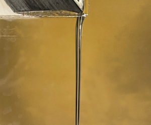
Figure 9 provides a sequence of standing wave observations for a flow rate of  $Q^\star = 1.23\ \text {cm}^2\ \text {s}^{-1}$. The sequence indicates that the $We_l=1$ condition is in fact achieved within the curtain (this occurs approximately 1 cm below the die) as per the previous discussion. Figure 10 provides a side-view image of the liquid curtain corresponding to this flow rate. It is clearly observed that the angle of the curtain centreline does not match that of the slot exit, namely $\alpha _i \neq \alpha _s$, and that the curtain shape is vertical downstream. Also observed is the underwetting of the lip with a slight interfacial curvature (the teapot effect; see Kistler & Scriven Reference Kistler and Scriven1994), indicating some flow rearrangement as anticipated by Weinstein et al. (Reference Weinstein, Ross, Ruschak and Barlow2019).

Figure 9. Standing wave observations for a volumetric flow rate of  $Q^{\star } = 1.23\ {\rm cm}^2\ {\rm s}^{-1}$ as (a–c) an obstacle is moved towards the die slot. Note that the standing wave breadth approaches the horizontal ( $\theta \to {\rm \pi}/2$; see also figure 4) as the obstacle moves upwards in the curtain. Panel (c) shows the approximate location in the curtain where the local Weber number is equal to $We_l=1$, as the waves become nearly horizontal. The standing waves have been enhanced with red lines to facilitate their visualization.

Figure 10. Side view of the curtain shape corresponding to a volumetric flow rate of  $Q^{\star } = 1.23\ {\rm cm}^2\ {\rm s}^{-1}$ and a subcritical ( $We_l < 1$) to supercritical ( $We_l > 1$) flow transition, as evidenced by the standing waves in figure 9. After entrance region adjustments, the curtain becomes vertical, the centreline at its top having a different angle from that of the slot.
The distinctly different flow behaviour for supercritical ( $We > 1$) and subcritical ( $We < 1$) regimes was observed for all flow conditions examined in the experiments. In supplementary material available at https://doi.org/10.1017/jfm.2023.811, we provide two videos documenting the sequence of shapes traversed by the curtain as the flow rate is varied in the range $Q^\star \in [1.23,3.7]\ \text {cm}^2\ \text {s}^{-1}$. The videos clearly show the transition from angled ( $We_l>1$ everywhere in the curtain) to vertical ( $We_l=1$ in the curtain) shapes. In the range of conditions surveyed experimentally, no upward-bending liquid curtains have been observed.
4.2. Two-dimensional viscous simulations at low Reynolds number
To expand on the range of conditions examined experimentally, 2-D viscous numerical simulations were performed by means of the BASILISK code. Table 1 summarizes the dimensional quantities employed in the simulations shown in figure 11, for three cases of supercritical regime ( $We > 1$), and one case of subcritical regime ( $We < 1$). Table 2 reports the corresponding dimensionless parameters. Note that the Reynolds number is $Re = O(1)$ for all cases, to simulate curtain flows of practical (experimental) occurrence. Indeed, high-Reynolds-number flows are typically avoided in precision coating operations to reduce the propensity for disturbance propagation; they are highly laminar in practice (Weinstein & Ruschak Reference Weinstein and Ruschak2004), and typical Reynolds numbers satisfy $Re<10$ (Schweizer Reference Schweizer2021).
Table 1. Dimensional physical quantities used in the 2-D numerical simulations reported in § 4.2.


Figure 11. Numerical 2-D curtain shape represented in terms of volume fraction  $C$ contour maps ( $C=1$ in the liquid phase, $C=0$ in the gas phase) by varying the Weber number: $We=5.42$ (a); $3.95$ (b); $3.07$ (c); (d) $0.77$ (see also table 2). Note that the top-left white region in all panels is outside the computational domain.
Table 2. Dimensionless governing parameters used in the 2-D numerical simulations reported in § 4.2. Note that  $Re$,
$Re$,  $Fr$ and $We$ are varied by changing the inlet velocity $U^\star _i$ (see table 1).

The supercritical curtain shapes are reported in figures 11(a)–11(c), for  $We=5.42$, 3.95 and 3.07, respectively. The subcritical shape corresponding to $We=0.77$ is shown in figure 11(d). The curtain shapes are represented in terms of volume fraction $C$ contour: the liquid phase is depicted in yellow (volume fraction $C=1$), the gaseous phase in blue ( $C=0$). Note that the top-left white region in all panels is outside the computational domain, and that the spatial coordinates have been scaled with respect to the curtain inlet thickness, namely $x = x^\star /H^\star _i$ and $y= y^\star /H^\star _i$.
For all the supercritical simulations, the initial slope of the curtain centreline exhibits an angle that coincides with that of the inlet slot ( $\alpha _i = \alpha _s=-50^\circ$). Overall the curtain shape follows the (expected) parabolic-like ballistic trajectory, with the ballistic range decreasing as the Weber number diminishes. This is due to the effect of surface tension, which pulls the curtain towards the vertical direction. These shapes qualitatively agree with the supercritical experimental evidence previously shown in figure 8, as well as those provided in the supplementary movies.
The 2-D simulation of the subcritical case  $We=0.77$, reported in figure 11(d), shows that the curtain approaches a vertical shape moving downstream ( $y < -40$). In a relatively small region around the inlet slot, the combined effects of viscosity and surface tension are responsible for the teapot effect (Kistler & Scriven Reference Kistler and Scriven1994). In this region, the flow rearrangement is such that the angle of the curtain centreline is not equal to that of the die slot, precisely in agreement with the experimental finding already shown in figure 10. Therefore, 2-D viscous simulations confirm the absence of upward-bending effect in the subcritical regime.
It is worth noting that the subcritical regimes characterized by the teapot flow were already observed by Keller & Weitz (Reference Keller and Weitz1957) in crude experiments. Those authors, as well as Benilov (Reference Benilov2023), attribute the impossibility of observing the upward-bending behaviour to the unstable nature of the solution. Our experimental and 2-D simulation results indicate, however, that any potential upwards bending is inhibited by the viscous flow rearrangement near the slot.
4.3. The 2-D numerical and 1-D modelling results in the inviscid limit
We now broaden the range of Reynolds number and Froude number in the exploration of possible solutions. In particular, we focus on low-gravity (high  $Fr$) and inviscid (high $Re$) regimes, that are not accessible in our experiments. To do so, we first validate the 1-D inviscid model predictions in this regime by detailed comparisons with the 2-D simulations. Once established, the 1-D model suffices to explore trends.
Figure 12 shows a typical comparison between the curtain shape predicted by the 1-D inviscid model (dashed red curve) and the curtain centreline extracted by 2-D viscous simulations. In particular, the 2-D results have been obtained by enforcing as an inlet boundary condition either a fully developed parabolic (Poiseuille) velocity profile (3.3a) (continuous black curve) or a plug inlet velocity profile ( $u=1$; continuous blue curve); both are chosen to have the same average velocity at the slot. The Reynolds number in the 2-D simulations is $Re=413$, a value that is sufficiently high to simulate the inviscid limit. In both the 1-D and 2-D cases, the Weber number is $We=2.5$. Overall, a good agreement can be observed between the 1-D and the 2-D plug solutions. Note also that, for the Poiseuille inflow boundary condition, the curtain centreline features a larger (approximately 30 %) ballistic deflection. As discussed previously, this discrepancy demonstrates the important effect of viscous relaxation near the slot. The 1-D inviscid model assumes that the flow is plug across the film at each arc-length location $s^\star$ (figure 5). When a plug flow is applied in the numerical simulation at the top of the curtain, there is little flow rearrangement required downstream as the effects of viscous traction at the slot walls are minimized. However, when a parabolic profile having the same average velocity at the slot as for the plug flow is implemented, there is significant vorticity in the flow that needs to dissipate before the inviscid model is valid downstream. Although not shown here, we have established that the inviscid 1-D model can be brought into agreement with the 2-D simulation with the parabolic profile by adjusting the magnitude of the plug velocity profile in the 1-D model at the slot. This adjustment may be viewed as the effect of the viscous entrance region on the reference velocity used in the inviscid 1-D model. The agreement between the 1-D model and 2-D simulation shown in figure 12 is typical of all other cases we have surveyed.

Figure 12. Effect of the inflow velocity boundary condition on the 2-D simulation compared with the 1-D model prediction. The solid curves represent the 2-D curtain centrelines for  $We=2.5$ and $Re=413$.
With the 1-D model thus validated, we can use its predictions to survey the parameter space more fully. Figure 13 illustrates the influence of the Weber number on the 1-D curtain shape for cases of low and high Froude numbers,  $Fr$=10 and $Fr=1000$, in figures 13(a) and 13(b), respectively. The high-Froude-number regime is particularly relevant, because the previous analysis by Benilov (Reference Benilov2019) considered the case of low gravity as a favourable physical scenario for the upwards bending of the curtain. All the curves reported in figure 13 are physically consistent. For both $Fr$ values, the absence of surface tension ( $We=\infty$) determines a curtain shape exactly reproducing the standard parabolic trend of the ballistic bullet. In low-gravity conditions ( $Fr=1000$), the high inertia effects inhibit the presence of high curvatures with respect to the lower-Froude-number case ( $Fr=10$), therefore mitigating the influence of the surface tension. Note that the curtain assumes the vertical behaviour as soon as the Weber number drops below unity; for all other $We$ subcritical values, the curtain shape remains vertical.

Figure 13. One-dimensional model prediction of the curtain centreline by varying  $We$ for two values of the Froude number: $Fr=10$ (a); $Fr=1000$ (b).
4.4. Influence of inlet boundary conditions in subcritical regime
As anticipated in § 3.2, the boundary conditions play a crucial role in predicting the curtain behaviour in the subcritical regime. Therefore, the boundary condition on the curtain location can be set, whilst the second one is that of removing the singularity at the critical location, i.e. where  $We_l=1$. This has been done analytically by Weinstein et al. (Reference Weinstein, Ross, Ruschak and Barlow2019), who found that the inlet curtain slope angle has to be $\alpha _i=-{\rm \pi} /2$, namely the curtain has to be vertical, regardless of the slot angle $\alpha _s$ and the subcritical Weber number $We$.
$We$.
In the current work, the 1-D model system (3.8a)–(3.12) is solved numerically in a different way from that of Weinstein et al. (Reference Weinstein, Ross, Ruschak and Barlow2019). The mathematical flexibility of the system enables two constraints to be applied at the top of the curtain. Therefore, we initially imposed that the curtain centreline angle is the same as that of the slot, i.e.  $\alpha _i=\alpha _s$ (via (3.10)–(3.11)), and that the location of the curtain centreline equals that of the slot, namely $y=0$ (via (3.12)). Results of the 1-D model integration performed using MATLAB are shown in figure 14(a,b) (figure 14b represents a magnification of figure 14a near the slot exit section), for a subcritical Weber number equal to $We=0.95$. The Froude number has been set to $Fr=10$. In particular, the red dashed curve corresponds to $\alpha _i = \alpha _s$. It is interesting to observe that the solver is robust enough to integrate through the singularity (i.e. the critical location), predicting a liquid curtain which is vertical everywhere except in a very small region near the slot. The region in which the curtain is not vertical lies within an arc-length distance that is only 1 % of the thickness of the curtain at its top; the tight curvature there does violate the slenderness assumption used to derive the 1-D model. For all curtain shape predictions in figure 14(a,b), it is found, however, that the momentum balance condition (3.13) used by Weinstein et al. (Reference Weinstein, Ross, Ruschak and Barlow2019) is not exactly satisfied at the critical location. This can be observed in figure 14(c), where the momentum imbalance error $\epsilon$, namely the difference between the right- and left-hand sides of (3.13), is plotted as a function of the boundary condition $\alpha _i$.

Figure 14. Curtain shape predicted by the 1-D model (a,b) and momentum imbalance error  $\epsilon$ in the critical location (c) by varying the curtain slope angle $\alpha _i$ in subcritical conditions. The vertical red dashed line in (c) denotes the value $\alpha _i=\alpha _s$. Here $We=0.95$, $Fr=10$.
Therefore, to improve the accuracy of the numerical solution at the critical location, the computation was repeated for both higher and lower curtain slope angles in the range  $\alpha _i \in [-{\rm \pi} /2,0]$. It has been found that the imbalance error $\epsilon$ consistently decreases as the curtain slope angle tends to $\alpha _i =-{\rm \pi} /2$, which is the only value giving $\epsilon =0$ (figure 14c). This is, in fact, a vertical liquid curtain (blue solid curve in figure 14a,b). Note that the same trend has been obtained for all subcritical $We$ and $Fr$ values we surveyed.
In summary, regardless of the Weber number, 1-D model curtain shapes issue vertically from the slot when the flow is subcritical. This result agrees with the recent theoretical finding by Weinstein et al. (Reference Weinstein, Ross, Ruschak and Barlow2019). While one can retain the condition on the curtain location at the inlet, the other condition is reserved to remove the singularity at the critical location. Therefore, via a different form of the same equations, the conclusion that the curtain must be vertical has been validated. It is interesting that the curtain inherently adopts a vertical shape immediately after the slot, even when numerical errors enable the imposition of the slope boundary condition. This indicates that the downward-falling vertical configuration is a stable solution.
5. Conclusions
The behaviour of an oblique liquid curtain exiting a non-vertical slot and falling under the influence of gravity, viscosity and surface tension has been investigated experimentally and theoretically. Experimental results have been theoretically confirmed through 2-D viscous numerical simulations performed by BASILISK, and by means of a simplified inviscid 1-D model. Apart from the technological relevance of this class of flows in the film coating process, one motivation of this work was to determine whether an upward bending of the curtain, predicted theoretically by Keller & Weitz (Reference Keller and Weitz1957) and Benilov (Reference Benilov2019), may be observed under subcritical conditions ( $We<1$ at the slot). We have found that when $We<1$ at the slot, an oblique liquid curtain attains a vertical shape everywhere except in a relatively small region around the slot where the curtain is formed. There, viscous flow rearrangement produces the characteristic teapot effect as is prevalent in many coating flows. The vertical result agrees with the recent theoretical finding by Weinstein et al. (Reference Weinstein, Ross, Ruschak and Barlow2019), who proposed the impossibility of prescribing a slope boundary condition on the curtain centreline at the slot exit when the die slot is inclined. The slope boundary condition, appropriate for a 1-D model, is that the curtain must be vertical regardless of the angle of inclination of the slot when the fluid leaves a slot under subcritical conditions. This is precisely the condition needed to remove a singularity in the curtain that arises at the critical location, namely where the local Weber number is 1. Note that we have not observed upward-bending curtains in our wide parameter survey. Finally, we have once again established the suitability of 1-D inviscid curtain models to match 2-D simulation predictions with appropriate parameter adjustments for viscous relaxation near the slot exit.
Supplementary movies
Supplementary movies are available at https://doi.org/10.1017/jfm.2023.811.
Acknowledgements
The 2-D numerical simulations included in the present work were performed on resources granted by CINECA under the ISCRA-C project HONOUR-2. S.J.W. would like to acknowledge insightful preliminary discussions with Dr D. Ross that helped to motivate this study.
Declaration of interests
The authors report no conflict of interest.


