


1. Introduction
Structures within glacier ice, including accumulation layers visible as primary stratification and secondary features such as crevasses, crevasse traces, folded layers, and longitudinal foliation, have been investigated for over a century to reconstruct deformation fields and motion within glaciers (see reviews by Hambrey and Lawson, Reference Hambrey, Lawson, Maltman, Hubbard and Hambrey2000; Hudleston, Reference Hudleston2015; Jennings and Hambrey, Reference Jennings and Hambrey2021). Such studies are also used to infer the transport pathways of englacial debris, which can accumulate by avalanching in the accumulation area, by falling into crevasses, or by being entrained into debris-rich basal ice layers that have been elevated from the glacier bed into an englacial, or even supraglacial, position (Hubbard and Sharp, Reference Hubbard and Sharp1995; Hambrey and Lawson, Reference Hambrey, Lawson, Maltman, Hubbard and Hambrey2000; Wirbel and others, Reference Wirbel, Jarosch and Nicholson2018). The few measurements of englacial debris concentration that have been reported indicate that debris-covered glaciers have higher concentrations than clean-ice valley glaciers (Bozhinskiy and others, Reference Bozhinskiy, Krass and Popovnin1986; Miles and others, Reference Miles2021). This is significant because englacial debris exhumation directly influences supraglacial debris thickness over the lower glacier (Kirkbride and Deline, Reference Kirkbride and Deline2013), thereby determining the spatial pattern of future surface ablation (Østrem, Reference Østrem1959). Supraglacial debris layers are expected to increase in thickness and to extend up-glacier over time as glaciers lose mass (Kirkbride and Warren, Reference Kirkbride and Warren1999; Scherler and others, Reference Scherler, Wulf and Gorelick2018). Understanding how these layers are produced and subsequently evolve is therefore important for the robust projection of future debris-covered glacier behaviour (Rounce and others, Reference Rounce2021; Rowan and others, Reference Rowan2021).
Structural glaciology has traditionally focused on mapping at the surface of glaciers and, as such, almost all structural studies to date have examined clean-ice glaciers (Hambrey and Lawson, Reference Hambrey, Lawson, Maltman, Hubbard and Hambrey2000). In some such studies, for example in Svalbard, englacial structural features preserved evidence of formerly more active ice flow, implying century-scale changes in glacier dynamics and thermal regimes (Hubbard and others, Reference Hubbard, Glasser, Hambrey and Etienne2004; Hambrey and others, Reference Hambrey2005; Lovell and others, Reference Lovell2015). Both observations of glacier deceleration (e.g., Dehecq and others, Reference Dehecq2019) and glacier modelling (Rowan and others, Reference Rowan2021) indicate that Himalayan debris-covered glaciers have undergone recent dynamic changes, yet evaluation in terms of glacier structure remains elusive. This is largely due to the presence of supraglacial debris, which both obscures the surface of such glaciers, preventing effective surface mapping, and hampers subsurface geophysical exploration, e.g., using ground-penetrating radar (GPR). Some structural features can be observed in the faces of ice cliffs, but these exposures are limited in number, spatially variable across glacier surfaces, and commonly adjacent to supraglacial ponds (Watson and others, Reference Watson, Quincey, Carrivick and Smith2017), preventing safe access. Additionally, ice cliffs are limited in vertical height to several metres, restricting observations at depth and hence of features that may not extend to the glacier surface.
For the reasons outlined above, detailed structural observations on debris-covered glaciers, particularly in the Himalaya, are scarce. The absence of structural maps for the heavily debris-covered areas of debris-covered glaciers greatly inhibits empirical observations of ice flow patterns and englacial debris transfer. Instead, these processes must be inferred from glacier surface velocities and imperfect debris thickness datasets. However, by penetrating and extending below the supraglacial debris layer, borehole-based imaging has the capacity to address this knowledge gap. For example, borehole optical televiewing records high-resolution images of the glacier interior (Hubbard and others, Reference Hubbard, Roberson, Samyn and Merton-Lyn2008), and the technique has been used to identify and characterise structural features and measure ice and firn density within debris-free ice masses (e.g., Obbard and others, Reference Obbard, Cassano, Aho, Troderman and Baker2011; Hubbard and others, Reference Hubbard2012, Reference Hubbard2013, Reference Hubbard2016; Ashmore and others, Reference Ashmore2017). Roberson and Hubbard (Reference Roberson and Hubbard2010) combined optical televiewing with surface mapping to identify eight different types of structure at (clean-ice) midre Lovénbreen, Svalbard. These structures were continuous layering, foliation, fold structures, three types of fractures (transverse, arcuate, and oblique), englacial sediment layers raised from the bed, and supraglacial debris ridges.
The aim of this contribution is to: (i) assess the effectiveness of borehole optical televiewing in reconstructing the 3D structure of a debris-covered glacier; (ii) map englacial structural features within a Himalayan debris-covered glacier; and (iii) evaluate the degree to which englacial structures reflect changes in the dynamic regime of a debris-covered glacier tongue. To do this, we used an optical televiewer (OPTV) to log four boreholes drilled into the debris-covered area of Khumbu Glacier, Nepal. A small number of layers presented herein have previously been interpreted in terms of their sediment load (Miles and others, Reference Miles2021).
2. Field site and methods
2.1 Field site
The study glacier, Khumbu Glacier, Nepal (Fig. 1), is one of the few debris-covered glaciers that has had some surface structural mapping up-glacier of the debris-covered zone or where that cover is thin. For example, Fushimi (Reference Fushimi1977) mapped the debris-free zone between the glacier's icefall and its heavily debris-covered tongue (Fig. 1b). Interpreted structures included open crevasses at the base of the icefall, foliation, and a small number of thrust faults located at the boundary between the mid and lower glacier (Fushimi, Reference Fushimi1977). A set of wave ogives extending down-glacier from the base of the Khumbu Icefall (Fig. 1b) has also been described (Fushimi, Reference Fushimi1977; Iwata and others, Reference Iwata, Watanabe and Fushimi1980; Hambrey and others, Reference Hambrey2008), resulting from seasonal variations in the volume of ice transported through the icefall (Goodsell and others, Reference Goodsell, Hambrey and Glasser2002). A short distance down-glacier, these ogives increase in height and evolve into ice pinnacles or sails (Iwata and others, Reference Iwata, Watanabe and Fushimi1980; Hambrey and others, Reference Hambrey2008; Evatt and others, Reference Evatt2017). This transition is likely due to the higher melt rate of the ogive troughs – enhanced by the presence of a thin layer of debris (Østrem, Reference Østrem1959) – than their crests. However, to date, no mapping has been reported within Khumbu Glacier's heavily debris-covered zone towards the terminus that has been stagnant for at least several decades. Velocities on Khumbu Glacier are greatest (>1 m d−1) in the icefall, but decrease to 10–20 m a−1 in the mid glacier and ~ zero in the terminal 4 km (Rounce and others, Reference Rounce, King, McCarthy, Shean and Salerno2018; Altena and Kääb, Reference Altena and Kääb2020).

Fig. 1. Location figure. (a) Location of Khumbu Glacier, Nepal; and (b) of drill sites on the glacier, also labelled with the OPTV image log length at each site. The background is a Sentinel-2A image acquired on 30.10.2018 (Planet Team, 2017) and glacier contours are at 100 m intervals from 4900 to 6800 m a.s.l., created from the 2015 SETSM DEM (Noh and Howat, Reference Noh and Howat2015). The boundary between the Khumbu and Nuptse flow units follows Hambrey and others (Reference Hambrey2008).
2.2 Methods
Four boreholes were drilled with pressurised hot water at four sites located within the debris-covered area of Khumbu Glacier (Fig. 1b). These boreholes were logged by an OPTV during the 2017 and 2018 pre-monsoon ‘EverDrill’ field seasons (Table S1). Each borehole is identified by its location, with Site 1 located farthest down-glacier, Sites 2 and 4 in the middle of the debris-covered area (west and east sides, respectively) and Site 3 in the upper debris-covered area (Fig. 1b). Drilling details were summarised by Miles and others (Reference Miles2018, Reference Miles2019) and OPTV logging and image log preparation by Miles and others (Reference Miles2021). The image logs, varying in length between 20.1 and 148.7 m (Fig. 1b), were acquired from each borehole in both down and up directions (full, raw, up-direction OPTV image logs are provided in Figs S1–S4), at a vertical image resolution of ~1 mm per pixel and a horizontal resolution of ~0.22 mm per pixel (Miles and others, Reference Miles2021).
Planes in the ice appear as sinusoids in unrolled (2D) image logs (Fig. 2) (Hubbard and others, Reference Hubbard, Roberson, Samyn and Merton-Lyn2008; Roberson and Hubbard, Reference Roberson and Hubbard2010). Excluding continuous primary layering in the host ice, which was subsampled, all discrete sinusoids present within the logs were delineated in WellCAD software to obtain each plane's strike (reported using the right-hand rule) and dip. Image logs in both directions were analysed to maximise feature certainty due to the differing settings used across the logs (Table S1). In some sections of the logs (see Figs S1–S4), a distinctive pattern of crude near-horizontal banding resulted from the OPTV imaging through varying amounts of sediment-laden water (likely due to the fluctuating borehole width; Miles and others, Reference Miles2019), and was omitted from the analysis. Delineated sinusoids were categorised into five types of plane based on visual and structural similarities, and eigen analysis was calculated on the poles to planes using Stereonet software (Allmendinger and Cardozo, Reference Allmendinger and Cardozo2019), with the primary eigenvalue presented as an indication of the strength of orientation clustering. To facilitate comparison with structures mapped in the glacier's middle and upper tongue in 1973, we locate the nearest individual appropriate layer mapped by Fushimi (Reference Fushimi1977) to each of our boreholes.
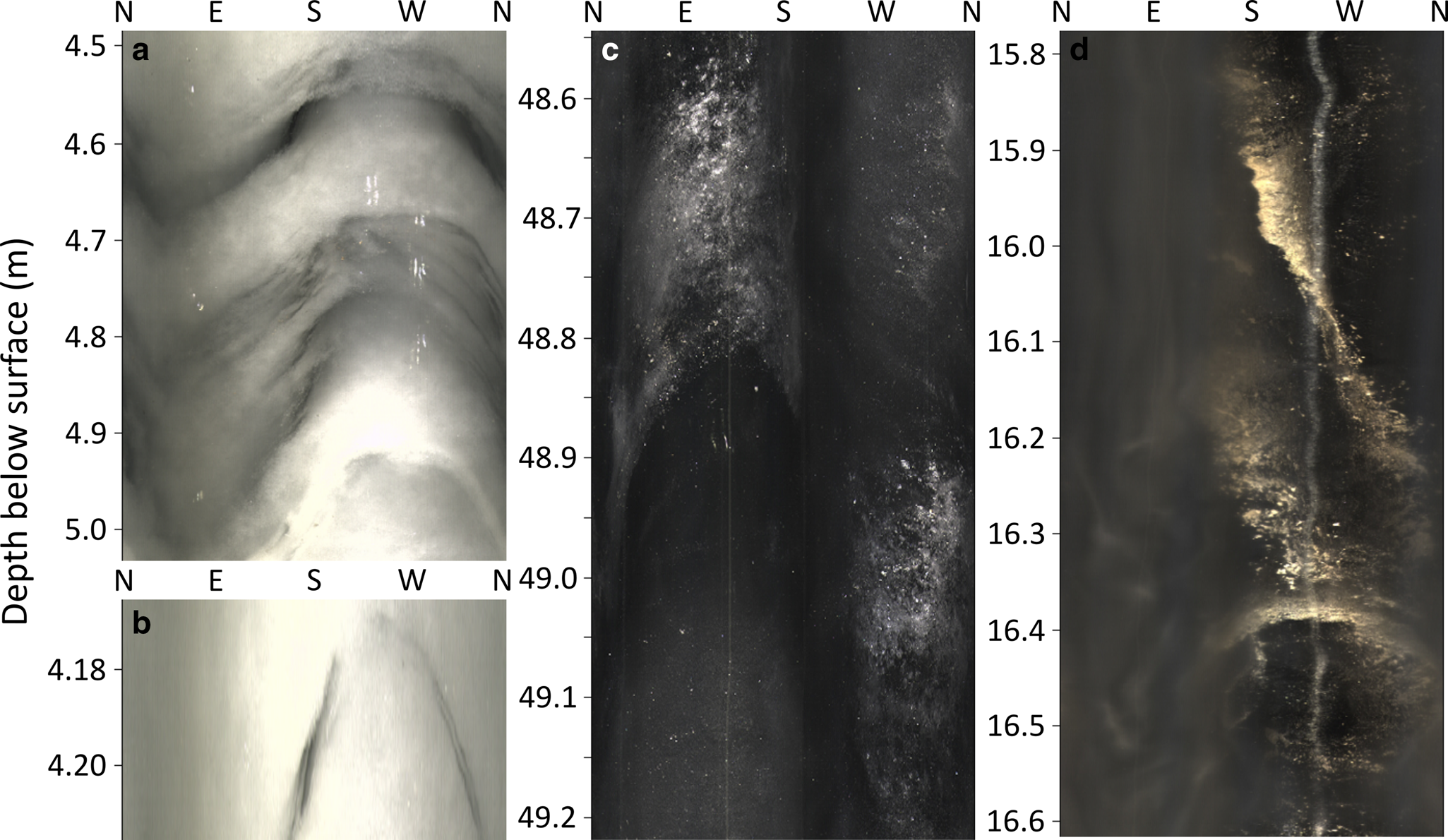
Fig. 2. Examples of planes, appearing as sinusoids in the unrolled OPTV image logs. (a) regular, alternating dark and light-coloured planes at Site 2; (b) a lighter-coloured layer within a darker-coloured plane at Site 2; (c) a bubble-rich ice plane from Site 4; and (d) steeply dipping planes comprised of fine sediment from Site 1. All logs are unrolled to progress North-East-South-West-North from left to right. Note the differing scales between the panels. Saturated vertical reflections and dark vertical traces are superficial artefacts from the drilling process.
3. Results
A total of 345.5 m of the glacier's interior was logged across the four boreholes. None of the boreholes were logged to the glacier bed: ice thickness is estimated to be 45 m at Site 1 (log depth 29.0 m) (Miles and others, Reference Miles2019), 200 m at Site 2 (log depth 20.1 m), 300 m at Site 3 (log depth 147.7 m), and 200 m at Site 4 (log depth 148.7 m; Fig. 1b, Table S1) (Gades and others, Reference Gades, Conway, Nereson, Naito, Kadota, Nakawo, Raymond and Fountain2000). Although image quality suffered in regions of turbid borehole water and from off-centre OPTV sonde alignment at Sites 1–3 (leaving vertical traces along the borehole wall; Fig. S5), there were still large sections of the image logs along which the borehole wall was visible with sufficient quality to reveal inclusions such as englacial debris (Miles and others, Reference Miles2021) and structural layers, allowing, to our knowledge, the first examination of englacial structures within a debris-covered glacier's tongue. The longest two logs (Sites 3 and 4; Figs S3 and S4) showed a reduction in luminosity with depth, which is common within OPTV image logs of glacier boreholes due to the reduction of light scattering as the bubble content of the ice decreases with depth (Hubbard and others, Reference Hubbard2013, Reference Hubbard2021).
As well as layering in the host ice (S0; Section 3.1 below), of which 249 layers were subsampled across regular depth intervals, 77 separate and distinctive planes (S1–S4; Sections 3.2–3.5 below) were identified and delineated across the OPTV logs (Table 1; full classifications are shown with the image logs in Figs S1–S4). While most planes appeared grey, a small number had a red-brown hue (e.g., Fig. 2d), identified as sediment and debris inclusions (Miles and others, Reference Miles2021). The five types of plane were coded in order of temporal evolution (see Section 4) according to standard convention (Hambrey and Lawson, Reference Hambrey, Lawson, Maltman, Hubbard and Hambrey2000) and are summarised below.
Table 1. Summary data relating to all mapped planes.

Plane frequencies for S0 at Sites 3 and 4 are the mean of frequencies calculated from five 1 m-long logged sections. The 95% CI column gives the 95% confidence interval in the angle of the plane's orientation.
3.1 Near-continuous planes (S0)
The host ice at Sites 2, 3, and 4 was composed of alternating layers of dark and light ice, designated S0 (Table 1; Figs S1–S4). Only one of these planes, located at Site 4, deviated in appearance in that it included a high concentration of small, white inclusions (Fig. 2c), interpreted as a particularly high concentration of bubbles. The mean thickness (± one std dev.) of the S0 planes was 25.1 ± 38.7 mm, ranging between sites from a mean thickness of 7.9 ± 10.7 mm at Site 2 to 30.7 ± 49.7 mm at Site 4 (Table 1). The estimated mean frequency of the S0 planes was 1.89 m−1 at Site 2, 4.80 m−1 at Site 3, and 5.40 m−1 at Site 4 (Table 1). The mean strike of the S0 planes was 267.3° across all sites: 329.6° at Site 2, 348.0° at Site 3, and 205.2° at Site 4. The mean dip of the S0 planes was 38.0° across all sites: 43.8° at Site 2, 71.1° at Site 3, and 67.9° at Site 4 (Table 1 and Fig. 3). The high primary eigenvalues, e.g., 0.95 and 0.85 at Sites 4 and 2, respectively (Table 1), demonstrate a strongly clustered (poles to planes) orientation.

Fig. 3. Planform outline of Khumbu Glacier with Schmidt lower-hemisphere equal-area plots of all poles to planes, classified by plane type. Poles to planes are plotted as solid circles, coloured and contoured by plane type (Kamb contour intervals of three standard deviations). Primary eigenvectors of the poles to planes, grouped by plane type, are plotted as diamonds. The poles to planes of the nearest foliation layers to each site measured by Fushimi (Reference Fushimi1977) are plotted as hollow triangles. The boundary between the Khumbu Icefall and Nuptse flow units follows Hambrey and others (Reference Hambrey2008).
S0 planes at Sites 2, 3, and 4 all displayed consistent changes in strike and dip with depth (Fig. 4). The strike of the S0 planes rotated by up to 100° over 13 m depth at Site 2 (equivalent to an anticlockwise rotation of 7.5° m−1), by 60° over 134 m at Site 3 (anticlockwise rotation of 0.4° m−1), and by 25° over 145 m at Site 4 (clockwise rotation of 0.2° m−1; Fig. 4a). Dip decreased with depth at all sites: by 56° over 16 m at Site 2 (i.e., equivalent to −3.5° m−1), by 27° over 136 m at Site 3 (−0.2° m−1), and by 27° over 146 m at Site 4 (−0.2° m−1; Fig. 4b).

Fig. 4. Strike (a) and dip (b) plotted against depth for all S0 planes sampled at Sites 2, 3, and 4. Note the x-axis of (a) extends from 90° to 90° to avoid splitting the distributions.
3.2 Debris-rich planes (S1)
At all four sites, there were a number of planes that had a distinctive red-brown hue (e.g., Fig. 2d), designated S1. These layers comprised visibly distinguishable, generally small-sized debris clasts (giving their distinctive colouring). These planes were the second most prevalent plane type and the only plane type that was present in all four borehole logs (Table 1). The mean thickness (± one std dev.) of these layers was 17.8 ± 30.0 mm, ranging between sites from 2.6 ± 2.4 mm at Site 2 to 38.9 ± 49.0 mm at Site 3 (Table 1). The mean frequency of the S1 planes was 0.83 m−1 at Site 1 (yielding a mean plane separation of 1.2 m), 0.15 m−1 at Site 2 (mean separation 6.7 m), 0.11 m−1 at Site 3 (mean separation 9.2 m), and 0.09 m−1 at Site 4 (mean separation 11.4 m; Table 1). S1 was the dominant plane type at Site 1 (comprising 24 of 34 layers identified) but formed a much smaller proportion of the total at the other three sites. The mean strike of the S1 planes was 298.5° across all sites: 311.3° at Site 1, 311.2° at Site 2, 339.0° at Site 3, and 208.5° at Site 4. The mean dip of the S1 planes was 30.9° across all sites: 21.9° at Site 1, 44.6° at Site 2, 66.7° at Site 3, and 63.2° at Site 4 (Table 1 and Fig. 3). The high primary eigenvalues, e.g., 0.98 and 0.94 at Sites 2 and 4, respectively (Table 1), demonstrate a strongly clustered orientation.
3.3 Bisected planes (S2)
Eight planes, located only at Sites 2 and 3 and designated S2, comprised a narrow (millimetre-thick), lighter-coloured layer that bisected a darker-coloured layer, typically tens of millimetres thick (e.g., Fig. 2b). The mean thickness (± one std dev.) of the S2 planes was 6.5 ± 6.8 mm, ranging from 4.4 ± 3.9 mm at Site 2 to 20.8 ± 0.0 mm at Site 3 (Table 1). The mean frequency of the S2 planes was 0.35 m−1 at Site 2 (yielding a mean plane separation of 2.9 m), with four very closely spaced at 7.42–7.58 m depth (each separated by 0.04–0.07 m), and 0.01 m−1 at Site 3 (one plane in the 147.7 m borehole; Table 1). The mean strike of the S2 planes was 344.0° across both sites: 344.5° at Site 2, and 341.5° at Site 3. The mean dip of the S2 planes was 52.3° across both sites: 51.4° at Site 2, and 58.6° at Site 3 (Table 1 and Fig. 3). The high primary eigenvalues of 0.96 and 1.00 at Sites 2 and 3, respectively (Table 1), demonstrate a strongly clustered orientation.
3.4 Thin, dark planes (S3)
Three planes, all located at Site 2 and designated S3, were dark in colour and had a notably different strike compared to all other plane types at the same site. These three planes had a mean thickness (± one std dev.) of 3.5 ± 3.6 mm and a mean frequency of 0.15 m−1 (yielding a mean plane separation of 6.7 m; Table 1). The mean strike of the S3 planes was 241.0° and the mean dip of the S3 planes was 51.3° (Table 1 and Fig. 3). The high primary eigenvalue of 0.89 (Table 1) demonstrates a strongly clustered orientation.
3.5 Sediment planes (S4)
Ten planes, all located at Site 1 and designated S4, comprised very fine sediment with a similar red-brown colouring to the larger-sized clasts of the S1 planes. The mean thickness (± one std dev.) of these layers was 20.5 ± 11.6 mm (Table 1). The mean frequency of the S4 planes at Site 1 was 0.34 m−1 (yielding a mean plane separation of 2.9 m; Table 1) and increased with depth from 0.10 m−1 in the uppermost 10 m of the borehole to 0.53 m−1 in the lowermost 10 m. The mean strike of the S4 planes was 288.1° and the mean dip of the S4 planes was 25.5° (Table 1 and Fig. 3). The primary eigenvalue of 0.66 (Table 1) demonstrates a weakly clustered orientation.
3.6 Observed surface structures
Three types of structural features were observed during fieldwork on the surface of Khumbu Glacier. In some clean ice cliff faces on the glacier surface, occasional dipping (Fig. S6) and folded debris planes (Fig. S7) were observed, particularly between Sites 2 and 3. Also, near Site 2, a high-angle, debris-rich layer containing striated and faceted clasts was observed cropping out at the glacier surface, and was thus interpreted as a basal thrust (Miles and others, Reference Miles2021, their Fig. S8).
4. Interpretation
4.1 Primary stratification (S0)
Given the pervasive presence of S0 at Sites 2, 3, and 4 and the strongly clustered orientation indicated by the high primary eigenvalues (≥ 0.85; Table 1), the unit is interpreted as the remnant of primary stratification – formed originally as layers of snowfall in the accumulation area of Khumbu Glacier in the Western Cwm and tributaries such as the Nuptse basin (Fig. 1b). The alternating dark and light colouring of S0 primary stratification is interpreted as indicative of the season in which the ice formed. Ice appears darker due to a lower concentration of bubbles in the ice, and lighter due to a higher concentration of bubbles, suggesting each layer formed seasonally, similar to OPTV-imaged primary stratification elsewhere (Hubbard and others, Reference Hubbard, Roberson, Samyn and Merton-Lyn2008; Roberson and Hubbard, Reference Roberson and Hubbard2010). In contrast to mid-latitude and polar glaciers, monsoon-influenced subtropical glaciers such as Khumbu experience warm, wet summers, during which mass simultaneously accumulates at high elevations and ablates at low elevations, and cold, dry winters, during which little mass change occurs. Ice coring studies in the Himalaya measured lower δ18O values in summer monsoon layers compared to winter (e.g., Qin and others, Reference Qin2000; Thompson and others, Reference Thompson2000; Ginot and others, Reference Ginot2014), perhaps reflecting the elution of heavy isotopes, and we thus associate the darker, bubble-poor layers with formation during the summer monsoon (June to August) and the lighter, bubble-rich layers with formation during the winter (December to February).
The dip of S0 – mean of 38.0° across all sites, with the greatest mean dip at up-glacier Site 3 of 71.1° (Table 1 and Fig. 5) – is within the range of primary stratification observations recorded in the lower parts of other valley glaciers. For example, the dip of OPTV-derived primary stratification on the tongue of midre Lovénbreen, Svalbard, ranged from near horizontal to 71° (Roberson and Hubbard, Reference Roberson and Hubbard2010), and surface-derived measurements on lower Fox Glacier, New Zealand, recorded primary stratification dipping up to 85° in the lower icefall (Appleby and others, Reference Appleby, Brook, Vale and Macdonald-Creevey2010). The thickness of S0 layers (ranging from a mean of 7.9 ± 10.7 mm at Site 2 to 30.7 ± 49.7 mm at Site 4; Table 1) was generally less than that reported from glacier tongues elsewhere. For example, OPTV-viewed primary stratification layers on Glacier de Tsanfleuron, Switzerland, were typically 100 mm thick (Hubbard and others, Reference Hubbard, Roberson, Samyn and Merton-Lyn2008). This difference can be explained by some combination of: (i) accumulation differences between these glaciers; and (ii) sample locations along each glacier (with the Khumbu sites that contain S0 being located in the middle of the glacier). The fine scale of the OPTV-derived layers may also represent intra-annual variations in accumulation or ablation that might not be identified as such by structural mapping undertaken at the glacier surface.

Fig. 5. 3D view of Khumbu Glacier and the mean orientation of each plane type with a strongly preferred (clustered) orientation, at each site. The view direction of the 3D image and all borehole sections is from SW (225°) to NE (45°). The glacier image is from a Sentinel-2A scene acquired on 30.10.2018 (Planet Team, 2017). The elevation data and background hillshade are from the HiMAT mosaic DEM (Shean, Reference Shean2017). Borehole sections are shown at a vertical scale of 1:10. Vertical ordering of planes is based on unit ID. The boundary between the Khumbu Icefall and Nuptse flow units follows Hambrey and others (Reference Hambrey2008).
4.2 Debris layers conformable with S0 (S1)
S1 was present at all sites and comprised layers characterised by the presence of visible debris clasts. The orientation of the unit was indistinguishable from that of the local S0 planes, e.g., at Site 4, where the mean strike was 205.2° at an angle of 67.9° for S0 and 208.5° at an angle of 63.2° for S1 (Table 1; Figs 3 and 5). S1 is therefore interpreted as surface debris that was incorporated into the glacier by passive burial in the accumulation area, perhaps by rock avalanching from the hillslopes surrounding the Western Cwm or the upper Nuptse basin (Fig. 1b). This is consistent with observations at the surface of Khumbu in clean ice cliff faces (Fig. S6) (Hambrey and others, Reference Hambrey2008) and elsewhere (Hambrey and Müller, Reference Hambrey and Müller1978; Roberson and Hubbard, Reference Roberson and Hubbard2010). As S1 planes were only some millimetres to centimetres thick, they are likely to have formed at the distal edge of such layer deposits. We note that our hot-water drill would have been unable to penetrate debris layers thicker than some centimetres (Miles and others, Reference Miles2019, Reference Miles2021) and it is therefore likely that our sample of S1 is biased towards thinner layers.
4.3 Water-healed crevasse traces (S2)
S2 was present at Sites 2 and 3, and comprised a thin (~1 mm), light-coloured (hence bubble-rich) central lamination that was enveloped by two dark-coloured, bubble-poor layers each typically 1–10 mm thick (e.g., Fig. 2b). Previous studies of similar features have interpreted the bubble-rich layer to result from the freezing of water, typically in an open crevasse, where gas has been expelled as the water freezes at the advancing ice front – increasing the gas concentration to the point of supersaturation and bubble formation in the central (last frozen) part of the now-healed crevasse (Hambrey and Müller, Reference Hambrey and Müller1978; Hubbard, Reference Hubbard1991; Pohjola, Reference Pohjola1994; Fountain and others, Reference Fountain, Jacobel, Schlichting and Jansson2005; Jennings and others, Reference Jennings, Hambrey, Glasser, James and Hubbard2016; Hubbard and others, Reference Hubbard2021). S2 planes therefore likely represent the healed traces of crevasses that were once water-filled. The thickness of S2 planes (mean of 4.4 ± 3.9 mm and 20.8 ± 0.0 mm at Sites 2 and 3, respectively; Table 1) was generally smaller than other surface-based observations – typically a few centimetres and very occasionally up to a metre thick (Hambrey and Müller, Reference Hambrey and Müller1978). This may be due to the high OPTV resolution allowing thin crevasse traces to be imaged that might be overlooked by surface-based observations; Hubbard and others (Reference Hubbard2021) also observed millimetre-scale healed crevasse traces using a borehole OPTV at Store Glacier, Greenland.
The similarity between the strike of S2 (mean of 344.5° and 341.5° at Sites 2 and 3, respectively) and S0 planes (mean strike of 329.6° and 348.0° at Sites 2 and 3, respectively; Table 1, Figs 3 and 5) indicates that S2 originated as, or developed conformably with, S0 primary stratification. However, crevasses typically form approximately perpendicular to the principal direction of extensional strain (Hambrey and Lawson, Reference Hambrey, Lawson, Maltman, Hubbard and Hambrey2000; Hubbard and others, Reference Hubbard2021). Thus, for crevasses to form parallel to S0 primary stratification, the S0 ice must have been rotated to dip steeply – perhaps within the icefall – producing sub-vertical planes of weakness that were exploited by fracturing. Indeed, the steep dip of S0 at Site 3 (mean of 71.1°; Table 1) indicates substantial rotation within the Khumbu Icefall, and the dip of S2 is similar to all other local planes (e.g., mean of 51.4° compared to 43.8° for S0 at Site 2; Table 1). Glaciers with icefalls are particularly noted to contain crevasse traces with a range of orientations (Jennings and Hambrey, Reference Jennings and Hambrey2021).
4.4 Healed crevasse traces (S3)
S3 was only present at Site 2, comprising dark-coloured, bubble-free planes that were rotated an average of 88.6° anticlockwise compared to the orientation of local S0 (the mean strike of S3 was 241.0° at an angle of 51.3°, compared to a mean strike of 329.6° at an angle of 43.8° for S0 at Site 2; Table 1, Fig. 5). Compared to local S0, S3 planes were both thinner (means of 7.9 ± 10.7 mm and 3.5 ± 3.6 mm, respectively) and more intermittent (S3 mean spacing of 6.7 m compared to the near-ubiquitous S0; Table 1). Clear (i.e., bubble-free), centimetres-thick ice layers that contrast with the lighter colour of the host ice have elsewhere been interpreted as either tensional veins or traces of water-filled crevasses that have refrozen (Hambrey and Milnes, Reference Hambrey and Milnes1977; Hambrey and Müller, Reference Hambrey and Müller1978; Jennings and Hambrey, Reference Jennings and Hambrey2021). Crevasse traces that cut across the prevailing crevasse field have also been observed down-glacier of the icefall of Fox Glacier, New Zealand (Appleby and others, Reference Appleby2017). We suggest two possible mechanisms that could account for S3 layers not hosting a central bubble-rich lamination as seen in S2 water-healed crevasse traces (Section 4.3). The first is that they may have formed by mechanical closure without the freezing of a liquid water layer. The second is that the freezing of such a layer may have been sufficiently disturbed, likely by turbulent flow, so that gas was unable to build up in the remaining liquid reservoir during progressive freezing.
The contrasting orientation of S3 compared to S2 crevasse traces (which have been interpreted to form from weaknesses in S0 primary stratification layering during rotation and transport through the icefall; Section 4.3), indicates that the two units formed in different locations. Given the location of Site 2 (Fig. 1b), S3 crevasses are therefore likely to have formed in relation to one of the former tributary glaciers on the western side of the glacier, below the base of the icefall (Fig. 1b), resulting in the observed formation of S3 layers cutting across the pattern of S0 primary stratification.
4.5 Basally derived layers (S4)
S4 was only present at Site 1, near the glacier terminus, and comprised layers of fine sediment, dipping up-glacier at a similar angle to S1 planes at the same site (Table 1, Fig. 3). S4 planes were thicker than local S1 planes (mean of 20.5 ± 11.6 mm compared to 5.1 ± 6.1 mm, respectively; Table 1), and although around half as frequent as S1 (S4 mean spacing of 2.9 m, compared to 1.2 m for S1 at Site 1; Table 1), the frequency of S4 increased with depth (0.1 m−1 in the uppermost 10 m compared to 0.5 m−1 in the lowermost 10 m). We interpret the fine sediment that comprises S4 to have been derived from the glacier bed (Hubbard and others, Reference Hubbard, Cook and Coulson2009; Miles and others, Reference Miles2021). Such subglacial debris can become incorporated into ice at the bed of a glacier through several mechanisms, including freeze-on by meltwater, relegation, and supercooling and freezing within the subglacial drainage system (e.g., Weertman, Reference Weertman1961; Iverson, Reference Iverson1993; Lawson and others, Reference Lawson1998).
Once subglacial debris has been incorporated at the glacier base, there are several mechanisms by which such layers can be raised into an englacial position to form dipping planes akin to S4 (e.g., several planes dip up-glacier at > 70°; Table 1, Fig. 3), all involving longitudinal compression. Such compression causes ice thickening (e.g., Hooke, Reference Hooke1973; Hooke and Hudleston, Reference Hooke and Hudleston1978; Monz and others, Reference Monz, Hudleston, Cook, Zimmerman and Leng2022), which is commonly accompanied by folding (e.g., Moore and others, Reference Moore2013). Several authors have also invoked thrusting (e.g., Glasser and others, Reference Glasser, Hambrey, Etienne, Jansson and Pettersson2003), involving the elevation of debris-charged basal layers through brittle failure along a shear zone under conditions of particularly intense longitudinal compression (Hambrey and Lawson, Reference Hambrey, Lawson, Maltman, Hubbard and Hambrey2000). Indeed, thrusting has previously been hypothesised for Khumbu Glacier (Fushimi, Reference Fushimi1977; Hambrey and others, Reference Hambrey2008; Miles and others, Reference Miles2021). While the dips we record for S4 are broadly consistent with those reported for thrusts elsewhere (mean of 25.5°, with several planes dipping > 70° (Table 1, Fig. 3) compared to angles of 50–70° at Storglaciären, Sweden (Glasser and others, Reference Glasser, Hambrey, Etienne, Jansson and Pettersson2003)), we did not observe any evidence of displacement along S4 planes in this study. We are therefore unable to either confirm or refute the (present or past) raising of basal layers by thrusting at our borehole sites.
5. Discussion
5.1 Borehole optical televiewing as a tool to investigate the englacial structure of debris-covered glaciers
OPTVs have previously been used successfully to reveal the subsurface structure of clean-ice glaciers (e.g., Roberson and Hubbard, Reference Roberson and Hubbard2010; Hubbard and others, Reference Hubbard2021). However, debris-covered glaciers provide an additional set of challenges in terms of both borehole drilling (Miles and others, Reference Miles2019) and OPTV logging through potentially turbid borehole water. Yet, this application of OPTV logging at Khumbu Glacier has demonstrated that the approach provides an effective means of investigating the internal structure of these glaciers, revealing features such as layers representing individual years of anomalous climatic conditions (see Section 5.3) that might otherwise only be observable in limited areas of exposed ice on the glacier surface, such as ice cliffs. The sub-millimetre spatial resolution of OPTV image logs also allows planes to be imaged that are thinner than may be identified by surface mapping by eye, including S2 water-healed crevasse traces and fine-scale variations in S0 primary stratification. OPTV logging allows included debris to be associated with structural units; here, for both S1, comprising small clasts, and S4, comprising fine basal sediment. Finally, borehole OPTV logging allows geometrical variability in structural units to be reconstructed as a function of depth, a variability that is otherwise difficult to determine. Such site-specific information would usefully be supplemented by coring (although more logistically challenging again than drilling by hot water) and interpolated or extrapolated spatially by surface-based geophysical exploration such as through GPR. However, high-resolution GPR surveys across debris-covered glaciers are challenging due to inconsistent antennae coupling at the rough surface and energy loss associated with water located within and immediately below the supraglacial debris layer (e.g., Gades and others, Reference Gades, Conway, Nereson, Naito, Kadota, Nakawo, Raymond and Fountain2000).
5.2 Comparison with previous surface mapping at Khumbu Glacier
Some of our results can be compared with the presence and orientation of certain surface structures mapped in 1973 by Fushimi (Reference Fushimi1977) due to the reduced extent of the supraglacial debris layer in the 1970s. S0 stratification reported herein is equivalent to Fushimi's ‘foliation layers’, and S4 basally derived layers may be equivalent to Fushimi's ‘thrusts’. S0 is similar in both strike and dip to that of the nearest foliation layer reported by Fushimi (Fig. 3); for example, at Site 2 the mean strike and dip for S0 is 329.6° and 43.8° and the strike and dip of the nearest foliation layer is 325° and 39°, indicating that there has been no substantial strain rotation in the past 45 years at these sites. In contrast, farther up-glacier at Site 4, while the dip is similar, the mean strike of the S0 layers reported herein is rotated by an average of 90° anticlockwise from Fushimi's layer (Fig. 3). This is likely due, at least in part, to the closer location of Site 4 to the lateral moraine (Fig. 1b), and hence within the Nuptse flow unit (see Section 5.3). We did not intercept S4 at any locations close to where Fushimi interpreted thrusts, precluding a comparison of orientation. However, we did observe a layer hosting basal debris cropping out at the glacier surface near Site 2 (Section 3.6), i.e., close to the location of Fushimi's thrusts.
We are also able to make some comparisons with, and updates to, the conceptual structural model of Khumbu Glacier presented by Hambrey and others (Reference Hambrey2008). For example, our OPTV-based structural analysis is consistent with Hambrey's inferred shear zone near the base of the icefall and the elevation of subglacial sediment through thrust planes, though these thrusts appear to be less frequent at this location than suggested in their conceptual model. The avalanche-derived stratification with debris reported by Hambrey and others (Reference Hambrey2008), equivalent to our S0 and S1, dips more steeply in our borehole records (e.g., S0 dips at 71.1° at Site 3 and 43.8° at Site 2; Table 1) than the near-horizontal dip shown in Hambrey et al.'s conceptual model. This difference could result from their model relating to locally derived (near-surface) avalanched debris layers while our boreholes intersect debris layers at depth that were sourced in the glacier's accumulation area and which have deformed with primary stratification (S0) during and following passage through the icefall.
5.3 Glacier-scale trends in S0 and S1
Having formed in the Western Cwm, the presence of S0 and S1 through the upper to mid debris-covered area suggests that this layering is preserved through the icefall despite substantial rotation (i.e., to form S2 crevasse traces; Section 4.3). The strike of S0 and S1 shows that these units generally align towards parallelism with each site's proximal lateral moraine: i.e., striking SSW at Site 4 in the eastern Nuptse flow unit, and NNW at Sites 2 and 3 in the western Khumbu flow unit (Figs 3 and 5). It is difficult to determine from our OPTV image logs whether S0 is dipping primary stratification or longitudinal foliation. Longitudinal foliation has been interpreted as primary stratification that has been transposed under lateral compression, associated in particular with the merging of flow units within a confined glacier tongue (e.g., Hambrey, Reference Hambrey1975; Hambrey and Lawson, Reference Hambrey, Lawson, Maltman, Hubbard and Hambrey2000). Our boreholes may have intersected an intermediate stage in this process, which is supported by the planes approaching parallelism with the proximal lateral moraine (Figs 3 and 4).
The OPTV image logs reveal that the dip of S0 decreases with depth down each borehole, by as much as 56° over the ~20 m-long Site 2 borehole (Fig. 4b). The strike of S0 also changes, rotating by up to 100° (at Site 2) anticlockwise with depth at Sites 2 and 3, and ~25° clockwise with depth at Site 4 (Fig. 4a). This rotation and decrease in the dip of S0 primary stratification with depth provides potentially valuable calibration data for spatially distributed ice flow models of both debris-covered and clean-ice glaciers. The change in strike and dip with depth reflects the glacier's 3D cumulative strain field, including the impact of historic tributary glaciers joining the main Khumbu flow unit in the recent past, particularly on the glacier's western margin (Fig. 1b), such as at Site 2. For example, the particularly high rotation of S0 and S1 with depth at Site 2 (Fig. 4) likely reflects the influence of confluent ice derived from the Changri Nup and Changri Shar historic tributary glaciers at this location (Fig. 1b).
S0 was decreasingly distinguishable both down-glacier and towards the base of the longer boreholes (lowermost ~40 m of Site 3 and ~20 m of Site 4; Figs 4, S3, and S4), which is caused by bubble exclusion from highly deformed deeper and older ice (Hubbard and others, Reference Hubbard2021). S0 was not observed at all at Site 1 (Table 1 and Fig. S1) where the oldest and farthest-travelled glacial ice would be located (Konrad and Humphrey, Reference Konrad, Humphrey, Nakawo, Raymond and Fountain2000). Indeed, primary stratification is often unidentifiable at the terminus of valley glaciers (Hambrey and Milnes, Reference Hambrey and Milnes1977; Hambrey and Müller, Reference Hambrey and Müller1978), although englacial debris layers that formed in the accumulation area have been observed to remain parallel to S0 primary stratification (Jennings and others, Reference Jennings, Hambrey and Glasser2014). S1 at Site 1 may therefore give some indication of S0 patterns at the terminus, where S0 has been transformed beyond detection. In contrast, the particularly bubble-rich S0 plane observed ~48 m beneath the surface at Site 4 (Fig. 2c) is much younger, and may be a remnant of a year with exceptionally high accumulation and/or cold air temperatures. This instance demonstrates that individually extreme events or seasons can be preserved in englacial structures and revealed by OPTV logging (Section 5.1).
Folding of S1 (and hence also S0) observed in the middle of the debris-covered area (Section 3.6; Fig. S7) occurs during transport through the lower glacier. These folds may be associated with the boundary between the main Khumbu flow unit and the tributary Nuptse flow unit (Hambrey and Lawson, Reference Hambrey, Lawson, Maltman, Hubbard and Hambrey2000; Hambrey and others, Reference Hambrey2008). Such a process could also incorporate supraglacial debris into the glacier (Hambrey and others, Reference Hambrey2008), thereby contributing to the greater englacial debris content at Site 1 than at Sites 2, 3, and 4 (Miles and others, Reference Miles2021). While no obvious folding-related inversion was apparent in our OPTV image logs, such patterns may well have occurred and been masked or over-printed.
5.4 Changes in the dynamic regime of Khumbu Glacier
Raising basally derived debris into an englacial position, as for S4, occurs in regions of strong longitudinal compression (Hambrey and Lawson, Reference Hambrey, Lawson, Maltman, Hubbard and Hambrey2000). Although hitherto interpreted more widely across Khumbu Glacier (Fushimi, Reference Fushimi1977; Hambrey and others, Reference Hambrey2008), we only observe S4 in the Site 1 borehole, within a kilometre of the glacier's terminus where the ice has been stagnant for at least 30 years (Quincey and others, Reference Quincey, Luckman and Benn2009). Numerical modelling has shown that the glacier has detached dynamically at the active-stagnant transition (located near to the palaeoconfluence of Changri Shar and Changri Nup Glaciers), and that this likely occurred during the first half of the 20th Century (Rowan and others, Reference Rowan2021). S4 at Site 1 could therefore not have been produced at the active-stagnant transition, because there would have been no such transition when ice flow was last sufficient to transport the historic Site 1 location to its current location at the terminus (i.e., prior to the Little Ice Age at about 0.4 ka; Rowan and others, Reference Rowan, Egholm, Quincey and Glasser2015). We therefore propose that S4 at Site 1 was produced when the terminus, and likely the whole glacier, was substantially more dynamic than at present, generating higher compressive strain rates towards the terminus than in its current stagnant configuration.
While the mechanism by which S4 basally derived sediment layers were raised cannot be determined from our borehole OPTV image logs, we suggest that the abrupt change in velocity at the base of the icefall (Altena and Kääb, Reference Altena and Kääb2020) – particularly in the past when the glacier was more dynamic (Rowan and others, Reference Rowan, Egholm, Quincey and Glasser2015) – seems the most likely location to generate sufficient compressive strain to result in the high frequency of S4 layers now located at Site 1. Alternatively, it is possible that a recent period of glacier advance resulted in flow being impeded by the glacier's substantial terminal moraine, causing longitudinal compression near the terminus and thus raising these layers close to their present-day location. Regardless of mechanism, we interpret S4 as a relic of a glacier that was historically more dynamic. In contrast, the layer hosting basally derived debris we observed at the glacier surface near our Site 2 (Section 3.6) was located a few hundred metres up-glacier of the thrusts mapped by Fushimi (Reference Fushimi1977). The low velocities in this part of the glacier since Fushimi's study (Quincey and others, Reference Quincey, Luckman and Benn2009; Rowan and others, Reference Rowan2021) suggest minimal down-glacier advection and that this layer may well be a thrust that formed at the active-stagnant transition, which modelling predicts will remain active until physical detachment within the next 50–130 years of 2020 CE (Rowan and others, Reference Rowan, Egholm, Quincey and Glasser2015, Reference Rowan2020).
6. Conclusions
We have presented the first englacial structural glaciological study from a Himalayan, or indeed any, debris-covered glacier using image logs from a high-resolution borehole OPTV. We draw the following conclusions:
• Despite logistical challenges, OPTV logging has proven effective in reconstructing the 3D structural features of a debris-covered glacier. Using a borehole OPTV, we have imaged structural features up to an order of magnitude smaller than those traditionally observed at the glacier surface, detected layers indicative of individual years of anomalous climatic conditions, and revealed trends with depth that would be challenging, and perhaps impossible, to reconstruct from surface-based observations.
• The debris-covered tongue of Khumbu Glacier hosts at least five structural units: (I) S0 primary stratification; (II) S1 debris layers conformable with S0; (III) S2 water-healed crevasse traces; (IV) S3 healed crevasse traces; and (V) S4 planes of basally derived fine sediment.
• Ice flow through the Khumbu Icefall is coherent enough to allow identification, up to the middle of the debris-covered area, of S0 primary stratification and S1 debris layers that accumulated with snowfall in the glacier's accumulation area.
• Intense ice deformation, involving substantial rotation, of S0 primary stratification occurs during flow through the icefall. This also induces crevasses to open up conformably with S0, which later heal through the freezing of water, producing S2 water-healed crevasse traces.
• S3 likely represents healed crevasse traces formed against the pattern of S0 primary stratification and thus formed in a different location from S2 water-healed crevasse traces.
• S0 primary stratification both decreases in dip and rotates with depth towards a parallel orientation with the proximal lateral moraine. This transformation, along with the relict S4 layers observed at the now-stagnant terminus of the glacier, preserve evidence of a time when the glacier was more active, indicating a change in the dynamic regime of Khumbu Glacier after the Little Ice Age maximum ~400 years ago.
Supplementary material
The supplementary material for this article can be found at https://doi.org/10.1017/jog.2022.100
Data
All raw data are available from the UK Polar Data Centre (OPTV images: https://doi.org/10.5285/d80f5c86-89a7-46d6-8718-47e3d34ab368; general borehole information: https://doi.org/10.5285/a7f28dea-64f7-43b5-bc39-a6cfcdeefbda).
Acknowledgements
This research was supported by the ‘EverDrill’ Natural Environment Research Council Grant awarded to Aberystwyth University (NE/P002021), and the Universities of Leeds and Sheffield (NE/P00265X). Borehole drilling equipment was also supported by funds from a Capital Equipment grant from the Higher Education Funding Council for Wales awarded by Aberystwyth University. KEM was funded by an AberDoc PhD Scholarship (Aberystwyth University). AVR was supported by a Royal Society Dorothy Hodgkin Research Fellowship (DHF/R1/201113). We thank Himalayan Research Expeditions for organising the logistics that supported fieldwork in Nepal in 2017 and 2018, particularly Mahesh Magar for guiding, navigation, and fieldwork assistance. We acknowledge the support of Sagarmatha National Park and their assistance with permitting. We thank the Scientific Editor, Dr Dan Shugar, and two anonymous reviewers for improving the manuscript.
Author's contributions
DJQ conceived of and led, and BH and AVR co-led, the EverDrill project. BH led the hot-water drilling, to which KEM, DJQ, and ESM contributed. BH and KEM carried out the OPTV logging. KEM processed the data and wrote the manuscript. All authors contributed to the data analysis and editing of the manuscript.
Conflict of interest
The authors declare no competing interests.


 Open access