


1 INTRODUCTION
Many classes of stars are either known or presumed to be binaries and many astrophysical observations can be explained by interactions in binary or multiple star systems. This said, until recently duplicity was not widely considered in stellar evolution, except to explain certain types of phenomena.
Today, the field of stellar astrophysics is fast evolving. Primarily, time-domain surveys have revealed a plethora of astrophysical events many of which can be reasonably ascribed to binary interactions. These surveys reveal the complexity of binary interactions and also provide sufficient number of high quality observations to sample such diversity. In this way, new events can be classified and some can be related to well-known phenomena for which a satisfactory explanation had never been found. Binary star phenomena are thus linked to outstanding questions in stellar evolution, such as the nature of type Ia, Ib, and Ic supernovae, and hence are of great importance in several areas astrophysics.
Another recent and important discovery is that most main-sequence, massive stars are in multiple systems, with ~ 70% of them predicted to interact with their companion(s) during their lifetime (e.g., Sana et al. Reference Sana2012a, Kiminki & Kobulnicky Reference Kiminki and Kobulnicky2012, Kobulnicky et al. Reference Kobulnicky2012, Kobulnicky et al. Reference Kobulnicky2014). This discovery suggests that many massive star phenomena are related to the presence of a binary companion, for example, type Ib and Ic supernovae (Podsiadlowski, Joss, & Hsu, Reference Podsiadlowski, Joss and Hsu1992; Smith et al., Reference Smith, Li, Filippenko and Chornock2011a) or phenomena such as luminous blue variables (Smith & Tombleson, Reference Smith and Tombleson2015). Additionally, the recent detection of gravitational waves has confirmed the existence of binary black holes (Abbott et al., Reference Abbott2016d), which are a likely end-product of the most massive binary evolution.
Finally, we now know that planets exist frequently around main-sequence stars. Planets have also been discovered orbiting evolved stars, close enough that an interaction must have taken place. These discoveries open the possibility that interactions between stars and planets may change not only the evolution of the planet or planetary system, but the evolution of the mother star.
The fast-growing corpus of binary interaction observations also allows us to conduct experiments with stellar structure, because companions perturb the star. Examples are the ‘heartbeat stars’, which are eccentric binaries with intermediate orbital separation. At periastron, the star is ‘plucked’ like a guitar string and the resulting oscillation spectrum, today studied thanks to high precision observations such as those of Kepler Space Telescope, can be used to study the stellar layers below the photosphere (Welsh et al., Reference Welsh2011).
Alongside new observations, creative new methods exist to model binaries. One-dimensional stellar structure and evolution codes such as the new Modules for Experiments in Stellar Astrophysics (mesa) are used to model not just stellar evolution, but binary processes such as accretion. Multi-dimensional simulations able to model accurately both the stars and the interaction are currently impossible because of the challenge in modelling simultaneously a large range of space and timescales. However, great progress over recent years has been made in 3D hydrodynamics with 3D models of individual stars (e.g., Chiavassa et al. Reference Chiavassa, Freytag, Masseron and Plez2011, where important relevant physics is captured) and numerical techniques being refined and developed to be adopted for binary modelling (e.g., Ohlmann et al., Reference Ohlmann, Röpke, Pakmor and Springel2016a; Quataert et al., Reference Quataert, Fernández, Kasen, Klion and Paxton2016). These studies are part of a revival in the field of stellar astrophysics, the start of which may be observed in the increase by over a factor of 10 in citations to seminal binary interaction papers such as that of Webbink (Reference Webbink1984, Figure 1), well above the factor of 2.3 increase in the overall volume of astrophysics papers that has been witnessed between 1985 and 2015.
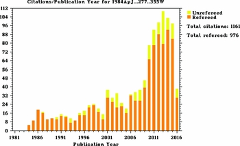
Figure 1. Citations to the seminal paper on the common envelope binary interaction of Webbink (Reference Webbink1984). The relative increase, starting in approximately 2006 cannot be explained by the overall increase in the number of astrophysics papers over the same period, demonstrating an increase in interest in this interaction over the last 10 years. Figure sourced from the Astrophysics Data Service.
This review is arranged as follows. We start with a summary of the properties of main-sequence binary populations (Section 2), including stars with planetary systems (Section 2.5). In Section 3, we briefly discuss binary pathways and list binary classes. In Section 4, we discuss current and future observational platforms particularly suited to the study of binary phenomena as well as modelling tools used to interpret observations and make predictions. We then, in Section 5, emphasise how certain classes of binaries allow us to carry out stellar experiments, whilst in Section 6 we report a range of interesting phenomena, which have been explained by including the effects of interactions between stars or between stars and planets. In Section 7, we discuss the exciting and expanding field of stellar transients, including the newly detected gravitational waves. We conclude in Section 8.
2 MAIN-SEQUENCE BINARY STARS
In this section, we summarise the frequencies of main-sequence binaries as well as their period and mass ratio distributions. For a recent review of stellar multiplicity in pre-main-sequence and main-sequence stars, see Duchêne & Kraus (Reference Duchêne and Kraus2013).
The fraction of stars that interact with their companions depends on these frequencies and on the action of tides and mass loss, which can both shorten and lengthen the orbital separation, bringing two stars within each other’s influence or allowing them to avoid an interaction altogether. Here, we define the binary fraction to be the fraction of systems that are multiple rather than the companion frequency, which can be larger than unity when there is more than one companion per primary on average.
We use the same naming conventions as Duchêne & Kraus (Reference Duchêne and Kraus2013). Massive stars are more massive than about 8 M⊙, intermediate-mass stars have masses from about 1.5 to 5 M⊙ (spectral types B5 to F2), Solar-type stars have masses in the approximate range 0.7 to 1.3 M⊙ (spectral types F through mid-K), low-mass stars between 0.1 and 0.5 M⊙ (spectral types M0 to M6), and very-low-mass stars and brown dwarfs are less massive than about 0.1 M⊙ (spectral types M8 and later).
2.1. The multiplicity fraction of main-sequence stars
Our knowledge of the fraction of massive stars that have companions was considerably revised by the Galactic O-star surveys of Sana et al. (Reference Sana2012a) and Kiminki & Kobulnicky (Reference Kiminki and Kobulnicky2012). Sana et al. (Reference Sana2012a) show that the fraction of O stars that have companions that will interact during the lifetime of the O star, i.e. with periods shorter than about 1500 d, is 71%. Of these, one-third merge. The overall binary fraction is established to be more than 60% in early B stars and in excess of 80% in O stars. There is evidence that the binary fraction in clusters and in the field are similar (Duchêne & Kraus, Reference Duchêne and Kraus2013).
The fraction of intermediate-mass stars in binary systems is substantially lower than for the most massive stars. Amongst the entire group of F2 to B5 type stars, the binary frequency is greater than about 50%, as determined from the Sco-Cen OB association (Kouwenhoven et al., Reference Kouwenhoven, Brown, Zinnecker, Kaper and Portegies Zwart2005; Fuhrmann & Chini, Reference Fuhrmann and Chini2012, Reference Fuhrmann and Chini2015).
As shown by Duquennoy & Mayor (Reference Duquennoy and Mayor1991) and, later, by Raghavan et al. (Reference Raghavan2010), about 44 ± 2% of G- and K-type main-sequence stars in the Solar neighbourhood have companions. They point out a low-significance difference of 9% between the immediately sub-Solar 41 ± 3% (G2–K3) and immediately super-Solar, 50 ± 4% (F6–G2) primaries.
The binary fractions of low- and very-low-mass stars are 26 ± 3% and 22 ± 5%, respectively (Duchêne & Kraus, Reference Duchêne and Kraus2013). These stars are not massive enough to evolve off the main sequence within the age of the Universe. They are thus more interesting as companions to more massive stars than as primaries in all but the closest binaries.
2.2. The period distribution of main-sequence binaries
The initial period distributionFootnote 1 of massive binaries has a peak at very short periods and declining numbers of larger period binaries out to a period of approximately 3 000 d. Two separate distributions are envisaged, a population of short period binaries (periods shorter than approximately 1 d) and a slowly declining power-law period distribution extending out to 10 000 AU (Sana et al., Reference Sana, Lacour, Le Bouquin, de Koter, Moni-Bidin, Muijres, Schnurr, Zinnecker, Drissen, Robert, St-Louis and Moffat2012b).
In intermediate mass stars of spectral type A and B, the initial period distribution lies between that of massive stars, which is a power law, and the longer period, log-normal distributions of Solar-like stars (Duquennoy & Mayor, Reference Duquennoy and Mayor1991; Raghavan et al., Reference Raghavan2010, see below). Indeed, Kouwenhoven et al. (Reference Kouwenhoven, Brown, Zinnecker, Kaper and Portegies Zwart2005, Reference Kouwenhoven, Brown, Zwart and Kaper2007) found that the observed intermediate mass binaries fit equally well a distribution flat in log-period (Öpik’s distribution). In fact, alone amongst all binaries, the A-type stars appear to present a double peaked period distribution with a peak below 1 AU and one at about 350 AU (Kouwenhoven et al., Reference Kouwenhoven, Brown, Zwart and Kaper2007; Duchêne & Kraus, Reference Duchêne and Kraus2013), although there is a great deal of uncertainty in these statements.
In Solar-like stars, the distribution is log-normal, peaked at about 104d (Raghavan et al. Reference Raghavan2010). This means that relatively few Solar-like binaries interact with their companions compared to more massive stars that are not only in binaries more often, but that have systematically closer companions.
Additional and updated information on the period distribution can be found in Moe & Di Stefano (Reference Moe and Di Stefano2016), who have reanalysed all existing binary observations.
2.3. The mass ratio distribution of main-sequence binaries
The more massive the companion relative to the primary, the greater the impact on the primary star once the binary interacts. Hence, the steeper the exponents, γ, of the mass ratio distribution (f(q) = q γ, where q = M 2/M 1 and M 1, 2 are the most and least massive component of the binary, respectively), the more dramatic the interactions in that population of binaries will be.
Equal mass binaries are not favoured in the massive star population (Sana et al., Reference Sana2012a), nor is there any evidence that the mass ratio distribution is different in wider and closer binaries (γ = −0.1 ± 0.6 at log P ≤ 3.5 and q ≥ 0.1 and γ = −0.55 ± 0.13 when a ≥ 100 AU). A peak in f(q) at q ≈ 0.8 does not point to a separate population of ‘twins’ (Lucy & Ricco, Reference Lucy and Ricco1979). A small population of high-mass ratio binaries could be due to mass-transfer during the pre-main-sequence phases.
Intermediate mass stars have a shallow mass-ratio distribution (γ = −0.45 ± 0.15) in both compact and wider binaries, although incompleteness remains a problem. Earlier claims that high-mass-ratio systems were favoured also in intermediate-mass stars, no longer seem to hold (Duchêne & Kraus, Reference Duchêne and Kraus2013).
The distribution of mass ratios in Solar-type stars is approximately flat (Raghavan et al. Reference Raghavan2010). Duchêne & Kraus (Reference Duchêne and Kraus2013) re-fitted the data of Raghavan et al. (Reference Raghavan2010) and found that longer period binaries (logP/d > 5.5) have a flat mass-ratio distribution (γ = −0.01 ± 0.03), whilst closer binaries (log P/d ≤ 5.5) have a higher incidence of components with similar masses (γ = 1.16 ± 0.16). There is a remarkable lack of substellar companions around Solar-type stars (the brown dwarf desert; Marcy, Cochran, & Mayor Reference Marcy, Cochran, Mayor, Mannings, Boss and Russell2000; Grether & Lineweaver Reference Grether and Lineweaver2006).
The situation is similar in low-mass stars. The mass ratio distribution is flat amongst the wide binaries, with γ = −0.2 ± 0.3 amongst systems wider than 5 AU (Duchêne & Kraus, Reference Duchêne and Kraus2013). Binaries closer than 5 AU have γ = 1.9 ± 1.7 as determined by fitting the data of the RECONS consortium (Henry et al., Reference Henry, Jao, Subasavage, Beaulieu, Ianna, Costa and Méndez2006). Brown-dwarf companions are easier to find around low-mass stars than around Solar-type stars. When brown dwarfs are the primaries in binaries, their companions tend to be of similar mass, suggesting a large γ (Burgasser et al., Reference Burgasser, Kirkpatrick, Cruz, Reid, Leggett, Liebert, Burrows and Brown2006).
Universally, multiplicity surveys are incomplete when q ≲ 0.1. As a result, in binaries with primary masses around 1 M⊙, the limit for detection of a companion is at the star-brown dwarf boundary. With only few brown dwarfs to be found around such stars, this bias may not result in a substantial underestimation of the number of companions around Solar-like stars. However, amongst stars more massive than 10 M⊙, the lack of information on binaries with q ≲ 0.1 means that the frequency of companions with mass as high as approximately 1 M⊙ is unknown. If an interaction with a much less massive companion results in a detectable change in the primary’s evolution, then we would like to know their numbers so as to account correctly for the frequency of these interactions.
Moe & Di Stefano (Reference Moe and Di Stefano2015) describe a handful of B-type stars with a very low-mass, pre-main-sequence companion. From these discoveries, they infer that B-type binaries with extreme mass ratios (q < 0.25) are in binaries only one third of the times of B-type binaries with more comparable masses (q > 0.25) for the same period range. They also conclude that the frequency of close, low-mass companions is a strong function of primary mass. This would render these low-mass companions unimportant to the binary evolution of Solar-type stars, but perhaps very important for more massive primaries as there are more of them.
Additional and updated information on the mass ratio distribution can be found in Moe & Di Stefano (Reference Moe and Di Stefano2016), who have reanalysed all existing binary observations.
This question can be extended to whether the interaction with a planetary mass companion would have any effect on the star. For example, would an interaction with Jupiter affect the evolution of the Sun? Planets are present around a substantial fraction of all main-sequence stars. If these planets do alter the evolution of their mother stars, then such interaction must be taken into account in stellar evolution (Section 2.5).
2.4. Orbital eccentricity of main-sequence binaries
Eccentricity is an important parameter in intermediate-mass systems. Recent studies, e.g., Tokovinin & Kiyaeva (Reference Tokovinin and Kiyaeva2016), suggest the number of stars, N, with a given eccentricity, e, is $\text{d}N/\text{de} \approx 1.2 e + 0.4$
, with a slight dependence on orbital separation. Close binaries probably tidally circularise prior to mass transfer by Roche-lobe overflow (Hurley, Tout, & Pols, Reference Hurley, Tout and Pols2002, see Section 3), but intermediate-period, eccentric binaries may undergo episodic mass transfer, which is as yet poorly understood (Sepinsky et al., Reference Sepinsky, Willems, Kalogera and Rasio2009; Lajoie & Sills, Reference Lajoie and Sills2011b). We discuss tidal circularisation further in Section 5.4.
$\text{d}N/\text{de} \approx 1.2 e + 0.4$
, with a slight dependence on orbital separation. Close binaries probably tidally circularise prior to mass transfer by Roche-lobe overflow (Hurley, Tout, & Pols, Reference Hurley, Tout and Pols2002, see Section 3), but intermediate-period, eccentric binaries may undergo episodic mass transfer, which is as yet poorly understood (Sepinsky et al., Reference Sepinsky, Willems, Kalogera and Rasio2009; Lajoie & Sills, Reference Lajoie and Sills2011b). We discuss tidal circularisation further in Section 5.4.
The distribution of the orbital eccentricity does not appear to depend on the mass of a binary system. Interestingly, it seems to be distributed similarly when companions are brown dwarfs or planets, showing that it is likely imparted by dynamical processes rather than star formation. In Section 2.6, we dwell further on orbital eccentricity because changes in its value at the hand of a second, wide companion can bring an inner companion, originally in an orbit too wide for interaction, into contact with the evolving primary.
2.5. Star–planet systems
Planets around main-sequence stars interact with the star if the orbital separation decreases or if the star expands to fill its Roche lobe (Section 3), provided that mass loss does not first widen the planetary orbit, reducing any chance of Roche-lobe overflow.
It is not clear how these interactions alter the evolution of the stars (Soker, Reference Soker1998b; Nelemans & Tauris, Reference Nelemans and Tauris1998; Nordhaus & Blackman, Reference Nordhaus and Blackman2006; Staff et al., Reference Staff, De Marco, Wood, Galaviz and Passy2016b). Effects of star–planet interactions may include spinning up of the star (e.g., Carlberg, Majewski, & Arras, Reference Carlberg, Majewski and Arras2009), pollution of the stellar envelope with materials from the planets (Sandquist et al., Reference Sandquist, Dokter, Lin and Mardling2002), increase of the mass-loss rate of the star in response to an interaction with the planet, or with its gravitational potential (Bear, Kashi, & Soker, Reference Bear, Kashi and Soker2011).
No planet has been observed plunging into a star even though such interactions must occur. If planets plunge into their star during its main-sequence phase, it is possible that only limited changes would be observed in the star. The most likely effect is the spin-up of the giant’s envelope (Privitera et al., Reference Privitera, Meynet, Eggenberger, Vidotto, Villaver and Bianda2016) whilst the enhancement of certain elements such as carbon, iron, or lithium is either modest of difficult to interpret due to various competing effects (Dotter & Chaboyer, Reference Dotter and Chaboyer2003; Privitera et al., Reference Privitera, Meynet, Eggenberger, Vidotto, Villaver and Bianda2016; Staff et al., Reference Staff, De Marco, Wood, Galaviz and Passy2016b). However, if particularly massive planets plunge into their star after the main sequence, when the stellar envelope is more extended and less gravitationally bound, it is possible that other effects may become observable. To plunge into the star when the star is extended, the planet needs to be at initial orbital separation between two and four times the radius the star has during its giant phases (depending on the strength of tides; e.g., Villaver & Livio Reference Villaver and Livio2009, Mustill & Villaver Reference Mustill and Villaver2012, Madappatt, De Marco, & Villaver Reference Madappatt, De Marco and Villaver2016). Unfortunately, techniques such as radial velocity variability or microlensing, which have yielded many planets (Sousa et al., Reference Sousa, Santos, Israelian, Mayor and Udry2011), only detect planets out to a few AU. Imaging surveys able to detect high contrast are few and have detected only a handful of planets out to tens of AU (Soummer et al., Reference Soummer, Brendan Hagan, Pueyo, Thormann, Rajan and Marois2011; Kuzuhara et al., Reference Kuzuhara2013). A handful of planets are also known around giant stars (e.g., Niedzielski et al., Reference Niedzielski2015), although these surveys are incomplete. As a result, there is no way, yet, to know how often planets orbit stars at distances such that the system will interact during the giant phases of the star.
There is some evidence that star–planet interactions may have taken place. For example, planets have been discovered in close orbits around stars whose precursor was larger than today’s orbit. Examples are the two earth-mass planets around KIC 05807616 (Charpinet et al., Reference Charpinet2011), which may be the disrupted cores of more massive gas giants (Passy, Mac Low, & De Marco, Reference Passy, Mac Low and De Marco2012b). All of these discoveries are indirect and there is a suspicion that at least some of them may be due to phenomena unrelated to the presence of a planet. A particular example is that of planets discovered around binaries that are known to have gone through a common envelope (CE) interaction (see Section 3). In most cases, the (indirect) detections of such planets have either been dismissed (Parsons et al. Reference Parsons2010) or the deduced planets’ orbits have been shown to be dynamically unstable, indicating that the observations are more likely to need an alternative explanation (Potter et al. Reference Potter2011; Hinse et al. Reference Hinse, Goździewski, Lee, Haghighipour and Lee2012; Horner et al. Reference Horner, Wittenmyer, Hinse, Marshall, Mustill and Tinney2013). In other cases, it appears that the planetary interpretation is the only one (e.g., NN Ser; Parsons et al., Reference Parsons2014), but that the planet was formed as a result of the binary interaction rather than at the time of star formation (Beuermann et al., Reference Beuermann2011; Veras & Tout, Reference Veras and Tout2012). Second generation planet formation remains an unexplored area of Astrophysics (Bear & Soker, Reference Bear and Soker2014), although we know that it must take place because of the presence of planets around some pulsars (Wolszczan & Frail, Reference Wolszczan and Frail1992).
2.6. Main-sequence triples and higher order multiple stars
The fraction of systems with a tertiary companion can be gauged by subtracting the fraction of multiples from the fraction of companions, whilst assuming that multiple systems comprise only binaries and triple systems. In Table 1 of Duchêne & Kraus (Reference Duchêne and Kraus2013), we see that the frequency of triples increases dramatically with primary mass from 0% in late-M stars and brown dwarfs to about half for stars more massive than 1.5 M⊙. Also, the closest binaries have tertiary companions far more often than wider binaries. Solar-type stars in binaries with periods shorter than 3 d have tertiaries in 96% of systems, compared to only 34% in binaries with periods longer than 12 d (Tokovinin et al., Reference Tokovinin, Thomas, Sterzik and Udry2006).
Table 1. Common names of classes of binaries and their likely interpretation (a ‘?’ denotes an uncertain interpretation).

Legend: MS = main sequence; WD = white dwarf; NS = neutron star; BH = black hole; CE = common envelope; SN = supernova; sdOB = subdwarf O or B; CEMP = carbon enhanced metal poor.
Such tertiary companions are of interest to stellar evolution because they may act to shorten the orbital period of the inner binary and alter the inner binary eccentricity. This can bring an inner binary initially too wide for an interaction during stellar evolution to within the reach of the expanding primary, therefore increasing the number of interactions in a population. For example, Hamers et al. (Reference Hamers, Pols, Claeys and Nelemans2013) find that in 24% of the triple systems they studied with a population synthesis technique, the inner binary, which initially is wide enough to avoid interaction, is hardened enough for mass transfer to start.
Finally, one of the most important reasons why we need to model mass transfer correctly is because it has an impact on the orbital elements, which in turn decide the strength and type of the interaction that follows. Whist analytical work has moved this field a long way (e.g., Sepinsky et al., Reference Sepinsky, Willems, Kalogera and Rasio2007, Reference Sepinsky, Willems, Kalogera and Rasio2009, Reference Sepinsky, Willems, Kalogera and Rasio2010; Dosopoulou & Kalogera, Reference Dosopoulou and Kalogera2016a, Reference Dosopoulou and Kalogera2016b), it is not clear how to implement this information in numerical codes (Staff et al., Reference Staff, De Marco, Macdonald, Galaviz, Passy, Iaconi and Low2016a; Iaconi et al., Reference Iaconi, Reichardt, Staff, De Marco, Passy, Price and Wurster2016). There, small stellar deformation or oscillations due to numerical artefacts translate into strong tidal torques that alter the orbit giving reasonable doubt that the orbital evolution (and hence the interaction) is well reproduced.
2.7. Binaries born in cluster environments
One of the fundamental questions of binary star formation is whether the binary frequency, period, mass ratio, and orbital eccentricity distributions are dependent on the birth environment. An obvious check is to compare these quantities for binaries in different clusters and in the field.
This is complicated by the fact that cluster environments, with a range of stellar densities, may alter the binary fraction and other characteristics of the binary population over time in different ways. The binary population thus carries the signature of its environment of birth, but also of the cluster’s age. Another caveat is that binaries in the field were born in different clusters that dissipated at different times. Hence, their binary characteristics would be a mix. Clearly, comparing binary populations in clusters and in the field is not easy, as there are many variables that contribute to their appearance, but this should not deter us from trying!
Recently, a thorough study of the binary population in M 35, a young, 180 Myr old cluster (Geller et al., Reference Geller, Mathieu, Braden, Meibom, Platais and Dolan2010), has revealed that the binary properties that could be probed by their study are similar to those of the binaries known in the field. More specifically, binaries and single stars show no difference in distribution within the cluster, and the binaries are not centrally concentrated. The binary frequency out to period of 104 d is 24 ± 3%, consistent with the binary frequency in the field to the same period limits (Duquennoy & Mayor, Reference Duquennoy and Mayor1991). This would argue that the field binary population is similar to that of a cluster that did not have time to alter the characteristics of its binaries. It seems also to argue that field binaries were not, on average, altered significantly whilst they inhabited their birth clusters.
In Section 3.3, we discuss how cluster dynamics change the binary population and contribute exotic binary formation.
3 BINARY EVOLUTION AND CLASSES: PATHWAYS AND NOMENCLATURE
A multiple star system has as many sets of stellar parameters—mass, metallicity, etc.—as there are stars in the system. In addition, there are parameters characterising the orbital elements, such as separation, eccentricity, spin alignment (Hut, Reference Hut1981), or orbital alignment in multiple systems. This large parameter space introduces complexity, particularly when the two or more stars interact, and two relatively similar systems may display quite diverse phenomenology.
Below, we summarise the types of binary interactions. We then compile a list of binary class names. Finally, we discuss how binary interactions play out in clusters, where encounters between stars and binaries are frequent.
3.1. Types of binary mass transfer
Binary classes can be best understood by thinking about the possible range of interactions that take place between two stars. The mass stored in a star is layered on equipotential surfaces. Stars remain spherical when they are small and compact, but as they age and expand their surfaces become distorted by the gravity of their companion star and by rotation which can be enhanced by tidal interactions with a companion. Distorted stars can sometimes be observed as ‘ellipsoidal variables’ (e.g., the sequence E stars; Nicholls & Wood Reference Nicholls and Wood2012, see Table 1 and Figure 2).

Figure 2. Period-luminosity diagram for evolved stars in the Large Magellanic Cloud. Sequence 1 consists of stars pulsating in the fundamental mode, whilst sequences 2 to 4 are higher order pulsational modes. Sequence E (Section 3.1; Table 1) stars are ellipsoidal binary systems, where a close companion distorts the giant primary star. The mechanism responsible for the variation on sequence D is not known. Credit: image adapted from figure 1 of Riebel et al. (Reference Riebel, Meixner, Fraser, Srinivasan, Cook and Vijh2010).
A special equipotential surface, called the Roche surface or Roche lobe, is shared between the two stars in a binary system. When one star expands beyond its Roche lobe, or the Roche surface shrinks into the star by loss of orbital angular momentum, any mass lying above the Roche surface can flow from one star to the other (Pringle & Wade Reference Pringle and Wade1985). This process is called Roche-lobe overflow.
The mass transfer naming convention is based on when, during its evolution, a star fills its Roche lobe. If mass transfer occurs during the core hydrogen burning phase of the donor, i.e. on the main sequence, it is called case A mass transfer. Alternatively, if mass transfer takes place whilst the donor is burning hydrogen in a shell, i.e. on the first or red giant branch (RGB), it is called case B. After helium ignition, e.g. on the asymptotic giant branch (AGB), mass transfer is referred to as case C.
Material that overflows can all be accreted by the companion, in which case the mass transfer is conservative. Alternatively, mass can be part accreted and part lost, a process called non-conservative mass transfer. If the accretor gains enough mass, the mass ratio can invert, with the originally more massive primary becoming the least massive and dimmer star. Such systems are known as Algols, named after the prototype for the class (β Persei, Table 1). The post mass-transfer distribution of Algol binary properties, such as orbital periods, is an important test of mass transfer efficiency (van Rensbergen et al., Reference van Rensbergen, de Greve, Mennekens, Jansen and de Loore2011, Section 4.2.1).
The evolutionary fate of a binary system depends crucially on whether the binary orbit shrinks or expands as a result of Roche-lobe overflow (Soberman, Phinney, & van den Heuvel, Reference Soberman, Phinney and van den Heuvel1997) and the response of the accreting star. When RGB or AGB stars expand and overflow their Roche lobe, they transfer mass to their companion (cases B and C mass transfer, respectively). If the accretor cannot accommodate the mass transferred to it, it too may fill its Roche lobe and a CE may form around the system (Section 4.2.2). A dynamical in-spiral phase follows, which typically results in a merger, or in the ejection of the CE and the emergence of a close binary, such as a sub-dwarf O or B binary, or the central star of a planetary nebula (Paczynski, Reference Paczynski, Eggleton, Mitton and Whelan1976; Ivanova et al., Reference Ivanova2013, Table 1; Section 6.3).
Mass transferred from one star to another carries angular momentum. Only about 10% of a star’s mass has to be accreted to spin the star to its break up rotation rate when it can accrete no more (Packet, Reference Packet1981). A combination of tidal interaction and wind mass loss can prevent a star from spinning this fast and allow it to accrete (de Mink et al., Reference de Mink, Sana, Langer, Izzard and Schneider2014). The excess angular momentum is transferred to the orbit by tides or lost in a wind. Tides also allow close systems, which undergo significant mass loss, to have rapidly spinning stars even until their death as supernovae and potential gamma-ray bursts (Izzard, Ramirez-Ruiz, & Tout, Reference Izzard, Ramirez-Ruiz and Tout2004; Detmers et al., Reference Detmers, Langer, Podsiadlowski and Izzard2008).
Magnetic fields are likely to alter the accretion pattern between two stars in at least some cases, particularly if the accretion is onto an evolved star, such as a white dwarf (WD) or a neutron star. The most well-known and extreme example is perhaps offered by ‘polars’ (Cropper, Reference Cropper1990, Table 1), where a highly magnetic WD (the record holder, AN Ursae Majoris, has a field of 2.3 × 10⁸ G) is accreting from a main-sequence companion. The accretion stream is channelled from the inner parts of the disk into the poles of the WD by the magnetic field or even directly onto the WD without the mediation of an accretion disk in the more extreme polars. Even more extreme are neutron stars accreting in high-mass X-ray binaries that have magnetic fields in the range 1011 − 13 G (e.g., Jaisawal & Naik, Reference Jaisawal and Naik2015).
Finally, a new type of Roche-lobe overflow has been recently added to the nomenclature: wind Roche-lobe overflow. In these binaries, the wind of the donor, for example, a mass-losing AGB star, has a velocity within a small range of values from the value of the escape velocity at the Roche surface of the donor. In such cases, even if the donor is not filling its Roche lobe, its wind naturally flows through the inner Lagrangian point and onto the accretor. This scenario was investigated by Mohamed & Podsiadlowski (Reference Mohamed, Podsiadlowski, Napiwotzki and Burleigh2007) in order to explain the peculiar observations of the AGB star Mira that is clearly transferring mass to a companion despite an orbital separation so large that Mira cannot be possibly filling its Roche lobe (Mohamed & Podsiadlowski, Reference Mohamed and Podsiadlowski2012).
3.2. A list of binary classes
Binary class nomenclature has arisen over the centuries in response to a range of binary discoveries achieved with a variety of observational techniques. Names have been coined for binaries discovered with a particular technique (e.g., radial velocity binaries), even when the systems detected are clearly a heterogeneous group from an evolutionary standpoint. As the wealth of binary interaction types started to emerge, classes that tried to divide the types of interactions emerged. According to the still oft-used Kopal (Reference Kopal1955) classification, binaries can be detached when neither star fills its Roche lobe, semi-detached when one star fills its Roche lobe or in contact when both stars fill their Roche lobe. Eventually, names emerged that collected objects thought to have evolved similarly (e.g., novae). This means that a given binary could be classified in more than one way (e.g., dwarf novae are semi-detached binaries).
In Table 1, we present a list of binary class names that have been used in the literature, alongside their current, best interpretation. We make no claim to completeness, nor do we dwell on each of these classes and on the subtleties of their interpretation. It is worth noting that a good classification system is one that is based purely on observed characteristics rather than interpretation. In Table 1, Sequence E stars are such an example. They appear on a specific locus of the period-luminosity diagram of Large Magellanic Cloud variables (Figure 2), something that will remain the case, irrespective of the interpretation we give them. On the other hand, binaries are too diverse a group of objects to enforce strict classification rules. Some objects will be grouped by virtue of being interpreted as having a common evolutionary origin based on a whole range of disparate observations, even if that interpretation may turn out to be incorrect later on.
3.3. Binary stars that evolve in clusters
Data on the binary populations of young clusters, such as those discussed in Section 2.7, are fundamental for choosing realistic initial conditions for N-body simulations of clusters. These allow us to determine the evolution of the binary properties in those environments to understand older cluster observations and to probe evolutionary channels for a range of compact cluster binaries, including the formation of cluster specific binaries such as certain types of blue straggler stars (Section 3.2). The binary population also affects cluster dynamics and cluster observables in general, such as the width of the main sequence in colour-magnitude diagrams.
Data on the binary properties of the young cluster M 35 have been adopted by Geller, Hurley, & Mathieu (Reference Geller, Hurley and Mathieu2013) as input to their N-body model of the much older cluster N 188 (7 Gyr; Meibom et al. Reference Meibom2009), under the assumption that the binary characteristics of N 188 when it was young were the same as those of M 35. This study has revealed a wealth of information regarding the way in which the cluster is environment alters the binary population and, conversely, how the binary population alters the overall cluster properties.
The cluster binaries of N 188 are segregated in the centre of the cluster both in observations (Geller et al., Reference Geller, Mathieu, Harris and McClure2008) and simulations. The binary frequency was chosen to be 27% (P < 104 d) at the start of the simulation, in line with 24% determined from observations of the young cluster M 35. This is extended in period to a total binary fraction of ~ 60%, which reduces to 53% within the first 50 Myr of the simulated cluster life. By 7 Gyr, the binary frequency is 33.5 ± 2.8%, only slightly larger than at the start and in line with observations of N 188 (29 ± 3%; Geller & Mathieu Reference Geller and Mathieu2012). Twins, binaries with mass ratio close to unity, are not input into the simulations nor are they produced dynamically, pointing to the formation of twins being a process of star formation. The main-sequence binaries largely maintain their characteristics throughout the 7 Gyr of cluster evolution (84% of the solar type binaries do not change their characteristics), although wider binaries (period longer than ~ 106.5 d) see their eccentricities increase over time. This may increase the number of binary interactions where the inner binary is perturbed by a tertiary in an eccentric orbit (Section 2.6).
Finally, the number of blue straggler stars in NGC 188 is much larger than the number of blue stragglers predicted by the N-body models of Geller et al. (Reference Geller, Hurley and Mathieu2013). The models predict that almost all blue stragglers in the cluster derive from stellar collisions. The models also predict too many WD-main sequence binaries with circularised orbits, but with periods longer than the tidal circularisation period. It is therefore thought that a different criterion should be chosen in the models so as to have fewer CE interactions that form WD-main sequence binaries, and more stable mass transfer interactions that would generate more mass-transfer blue stragglers. This could be a solution to both discrepancies between model and observations. Ultimately, we need a better description of mass transfer to inform population synthesis models of which binaries enter a CE phase and which do not (Sections 3.1 and 4.2.1).
4 THE BINARY STAR TOOLKIT
A few observational tools have been, or are at present, particularly useful to binary star observers. The radial velocity technique exploiting high resolution spectrographs such as the Fiber-fed Extended Range Optical Spectrograph (FAROS) (e.g., Setiawan et al., Reference Setiawan, da Silva, Pasquini, Hatzes, von der Luhe, Girardi, Guenther, Hilditch, Hensberge and Pavlovski2004) has been and will always be a tool of choice in studying binaries (and planets). Alongside this workhorse a host of new techniques and telescopes have been developed that present new types of evidence (Section 4.1).
As for models, we distinguish modelling codes and techniques into two categories which can function in unison. The first class numerically solves equations that describe the stars either hydrostatically or hydrodynamically. Individual binary systems are modelled over time and parameters such as the evolution of radius or luminosity, mass transfer rate, masses, and kinematics of forming disks or jets are output. The second class includes population synthesis models. These can be more or less complex but all aim to model population characteristics such as distributions of masses, luminosity functions, or outburst rates. We briefly review some of these tools below (Section 4.2).
4.1. The toolkit: observations and observatories
The Atacama Large Millimetre Array (ALMA), with its exquisite sensitivity and excellent spatial resolution, has resolved binary features such as spirals in giant star outflows caused by orbiting companions (Maercker et al., Reference Maercker2012, Figure 3). It also allows us to characterise further, and lend corroborating evidence to the phenomenon of wind Roche-lobe overflow (Section 3, also Vlemmings et al. Reference Vlemmings, Ramstedt, O’Gorman, Humphreys, Wittkowski, Baudry and Karovska2015). Large Keplerian disks around stars can be used to infer a binary past (e.g., Bujarrabal et al., Reference Bujarrabal, Castro-Carrizo, Alcolea, Van Winckel, Sánchez Contreras, Santander-García, Neri and Lucas2013) even when a binary companion is not seen. Finally, the detection of magnetic fields strengths and geometries in giant stars (e.g., Pérez-Sánchez & Vlemmings, Reference Pérez-Sánchez and Vlemmings2013) is a fundamental step to understand how they are generated and the interplay between duplicity and magnetic fields (Nordhaus & Blackman, Reference Nordhaus and Blackman2006; Nordhaus, Blackman, & Frank, Reference Nordhaus, Blackman and Frank2007).

Figure 3. Left panel: ALMA (Section 4.1) observation of the AGB giant R Sculptoris (Maercker et al., Reference Maercker2012). Credit: ALMA Observatory. Right panel: SPH hydrodynamic simulation of the system; the spiral wave requires a binary companion with a period of 445 yr sculpting the mass lost from the star. Credit: Shazreen Mohamed, SAAO.

Figure 4. A series of density slices at six different times along the orbital plane during a 3D, hydrodynamic simulations of a common envelope in-spiral (Section 4.2.2) of a 1-M⊙ companion in the envelope of a 2-M⊙ RGB star. The X marks the position of the companion, the plus symbol marks the position of the RGB star’s core. The insert shows a central region of approximately 20 R⊙. The colour scale ranges between 10−6 and 10−3 g cm−3. Credit: image adapted from Figure 3 of Ohlmann et al. (Reference Ohlmann, Röpke, Pakmor and Springel2016a).
Optical and near infrared interferometry has been particularly successful in the study of binaries. The Center for High Angular Resolution Astronomy (CHARA) Array, for example, resolved the orbit of double-lined spectroscopic binary 12 Persei (Bagnuolo et al., Reference Bagnuolo2006), allowing precise mass estimates that can later be used as calibrators of other systems. It was also used to resolve the inner orbit in hierarchical triples, including Algol systems (O’Brien et al., Reference O’Brien2011; Baron et al., Reference Baron2012), and even succeeded in resolving massive Wolf–Rayet (WR) type binaries (Richardson et al., Reference Richardson2016).
Interferometry carried out with the Very Large Telescope Interferometer (VLTI) was the one to resolve disks around post-AGB stars (Deroo et al., Reference Deroo2006, Section 4.2.2), not to mention a host of disks and tori nested inside the cores of pre-planetary nebulae (PNe) (e.g., Chesneau et al., Reference Chesneau2007) or in newly exploded stars thought to be the product of a merger (e.g., Chesneau et al., Reference Chesneau2014, Section 7). Today, thanks to Spectro-Polarimetric High-contrast Exoplanet REsearch, SPHERE, detailed observations are being taken of AGB systems such as LB Pup where a (presumed) binary causes a bipolar outflow (Kervella et al., Reference Kervella2015).
Also of note is the Kepler Space Telescope that stared at a small patch of sky reaching micro-magnitude variability detections. Kepler has had a tremendous impact on the characterisation of binaries. A large new catalogue of assorted eclipsing binaries was compiled (Prša et al., Reference Prša2011), subtle, rare, or previously unseen phenomena, like the heartbeat stars were discovered (Section 5.2), rotation rates were measured in post-CE WDs (Hermes et al., Reference Hermes2015) or in single WDs rotating so fast that they must be the product of mergers (Handler et al., Reference Handler, Prinja, Urbaneja, Antoci, Twicken and Barclay2013), the phenomenon of Doppler beaming was detected in close compact binary systems including some double degenerates (e.g., van Kerkwijk et al., Reference van Kerkwijk, Rappaport, Breton, Justham, Podsiadlowski and Han2010; De Marco et al., Reference De Marco, Passy, Frew, Moe and Jacoby2015). Finally, speckle interferometry has been useful to map a variety of binary stars, including the dusty environments of WR-O star binaries (Section 6.4.1).
Surveys capable of observing short-timescale, transient sources in great detail form a pillar of 21st century astronomy and directly affect binary star observations. These surveys observe in wavelengths from radio to gamma rays and hence probe objects in exquisite detail. They serve as early-time alert mechanisms for deep, multi-wavelength follow-up observations. Many binary star phenomena are directly accessible to these surveys, such as gamma-ray bursts, novae, stellar mergers, tidal disruptions, supernovae and, of course, gravitational waves, as will be discussed in Section 7.
4.2. The toolkit: modelling techniques and codes
4.2.1. Modelling binary interactions
Modelling a single star is a complex task, despite the fact that, by and large, the evolution of a single star is determined only by its mass, composition and rotation rate. With some reasonably well-justified simplifications, such as the assumption of spherical symmetry, hydrostatic equilibrium and the mixing length theory for convection, stellar evolution is tractable on reasonable timescales and a range of 1D stellar evolutionary codes exists. Ideally, binary interactions should be modelled in 3D, where both stars are modelled with the same accuracy as in 1D and where the interaction is tracked by solving the Euler equation using self-gravity, full radiation transport and magnetic fields. Such complexity is at the moment beyond the realm of possibility, because of the vast range of time and size-scales that needs to be resolved. Some of the codes and code families have been listed in Table 2.
Table 2. A list of some of the major computational programmes used in the study of binary evolution.

Code family: a Eggleton Reference Eggleton1971, b Kippenhahn, Weigert, & Hofmeister Reference Kippenhahn, Weigert, Hofmeister, Alder, Fernbach and Rothenberg1967, c Paczynski, d bse/sse, e SeBa/sse.
f AMR = adaptive mesh refinement; g SPH = smooth particle hydrodynamics.
Single star models using 3D hydrodynamic codes. Parts of (single) stars can be modelled in 3D, for example, to model convective and rotational mixing (Meakin & Arnett, Reference Meakin and Arnett2007; Cristini et al., Reference Cristini, Hirschi, Georgy, Meakin, Arnett, Viallet, Meynet, Georgy, Groh and Stee2015). Full 3D hydrodynamical models of stars have been constructed with the djehuty code at Livermore (Bazán et al., Reference Bazán, Turcotte, Keller and Cavallo2003), but they are extremely computationally intensive. 2D, hydrostatic stellar evolution is also starting to be explored as a natural stepping stone to full 3D modelling (Espinosa Lara & Rieutord, Reference Lara and Rieutord2013). Convection in giant stars was studied using 3D models by Meakin & Arnett (Reference Meakin and Arnett2007) and more recently by Chiavassa et al. (Reference Chiavassa, Freytag, Masseron and Plez2011) with co 5 bold (Freytag, Steffen, & Dorch, Reference Freytag, Steffen and Dorch2002) at relatively low resolution, but high enough for a meaningful comparison with VLTI observations of Wittkowski et al. (Reference Wittkowski, Chiavassa, Freytag, Scholz, Höfner, Karovicova and Whitelock2016). This revealed the size of the modelled convection plumes to be approximately correct. Herwig et al. (Reference Herwig, Woodward, Lin, Knox and Fryer2014) modelled hydrogen entrainment in giant stars in 3D revealing the need for 3D to model AGB thermal pulse nucleosynthesis.
Binary interaction models using 1D implicit codes. 1D stellar evolution codes are used to model binary interactions, with binary phenomena such as accretion accounted for after parameters such as the orbital separation and accretion rates are calculated analytically, or guided by separate simulations with 3D codes (see below). Many such codes exist, of which there are a few families. The Eggleton codes are based on the single-star code of Eggleton (Reference Eggleton1972). Unique features include a non-Lagrangian moving mesh, which reduces the computational time involved in converging a stellar model, with the inclusion of some unwanted numerical diffusion. Modern versions of this code include twin (Glebbeek et al., Reference Glebbeek, Pols and Hurley2008), stars, and bs (Stancliffe & Glebbeek, Reference Stancliffe and Glebbeek2008). All include mass transfer and tidal interactions, with the most modern version of bs also including magnetic field generation (Potter et al., Reference Potter, Chitre and Tout2012).
Another commonly used binary star code is based on the original Kippenhahn code, exemplified by the Bonn Evolutionary Code (bec, Heger, Langer, & Woosley Reference Heger, Langer and Woosley2000; Yoon et al. Reference Yoon, Woosley and Langer2010). This includes parameterised rotational mixing, magnetic fields, mass transfer, and tidal interactions. The binstar code of the (French-speaking) Brussels group (Siess et al., Reference Siess, Izzard, Davis and Deschamps2013) also derives from this original code base, although it has been updated to include, for example, the physics of mass transfer in eccentric systems (Davis, Siess, & Deschamps, Reference Davis, Siess and Deschamps2013). The Flemish-speaking Brussels group also has a binary star code, called the Population number synthesis (pns; De Donder & Vanbeveren Reference De Donder and Vanbeveren2004), which it uses for both detailed evolution and population synthesis (Section 4.2.3).
The newest addition to the selection of binary star codes is that of the mesa group (Paxton et al., Reference Paxton2015). This combines the widely used mesa single-star code with binary star physics. Amongst its advantages, mesa was designed from the beginning by a software engineer, so it is relatively easy to use and develop.
Binary interaction models using 3D hydrodynamic codes. Hydrodynamic models of binary interactions do exist, but they must make a number of simplifying assumptions and be guided by analytical considerations, in particular, if they include self gravity of the gas, something that will make simulations much slower. They represent the stars as simple hot spheres of gas in hydrostatic equilibrium. Example simulations are those of Lajoie & Sills (Reference Lajoie and Sills2011b) who modelled eccentric interactions between main-sequence stars, deriving parameters such as the time of maximum mass transfer rate compared to the time of periastron passage. These models can be compared with analytical models of this phase such as those of Sepinsky et al. (Reference Sepinsky, Willems, Kalogera and Rasio2009). The WD-WD merger simulations of Staff et al. (Reference Staff2012) carried out to simulate the formation of R Coronae Borealis stars from which merger temperatures and timescales can be interfaced with 1D stellar structure models to determine the nucleosynthetic signature of these mergers (Menon et al., Reference Menon, Herwig, Denissenkov, Clayton, Staff, Pignatari and Paxton2013).
A different class of binary interactions can be modelled without using self gravity of the gas, but where a gravitational field is imposed, such as that produced by an object embedded in the gas. Wind–wind collision models have been performed over the decades to understand all kind of phenomena associated with single stars (e.g., in PNe; García-Segura et al. Reference García-Segura, Langer, Różyczka; and Franco1999). Similar techniques can be adopted in the study of wind-wind collisions in binary systems such as for example, the collision between the wind of a WR star and that of an O star companion, as we describe in detail in Section 6.4.1. Hendrix et al. (Reference Hendrix, Keppens, van Marle, Camps, Baes and Meliani2016) listed the history of such models starting with the models of Stevens, Blondin, & Pollock (Reference Stevens, Blondin and Pollock1992) and ending with those of Bosch-Ramon, Barkov, & Perucho (Reference Bosch-Ramon, Barkov and Perucho2015). They also presented a model of the pinwheel nebula WR98a carried out with the code mpi-amrvac (Porth et al., Reference Porth, Xia, Hendrix, Moschou and Keppens2014). These models aim to study the wind interaction region as accurately as possible to understand how dust forms. Pinwheel nebulae are chief dust producers, despite the relatively hostile environments and understanding these interactions contributes to the larger understanding of the dust budget of the Universe. However, these simulations are not aimed at understanding the evolution of the binary per se, although without doubt such systems will have quite an interesting life as both the stars are due to explode as core collapse supernovae at some point.
Somewhat similarly, the simulations of Booth, Mohamed, & Podsiadlowski (Reference Booth, Mohamed and Podsiadlowski2016) using the SPH code gadget (Springel et al., Reference Springel2005) in the adaptation of Mohamed et al. (Reference Mohamed, Mackey and Langer2012) were used to study the circumstellar environments of symbiotic novae (WDs accreting from giant stars’ winds; Table 1). Such systems can in principle be progenitors of type Ia supernovae and their circumstellar environment could cause observed absorption line variability first observed in supernova type Ia 2006X (Patat et al., Reference Patat2007). The same code was used to simulate spiral shocks imprinted by a wide binary companion in a long orbit with an AGB star, as seen by ALMA in Section 4.1, see also Figure 3 (for a similar approach, see also the work of Kim & Taam (Reference Kim and Taam2012)).
A creative technique is that of using a range of different codes as well as analytical approximations in unison. An example is the work of de Vries, Portegies Zwart, & Figueira (Reference de Vries, Portegies Zwart and Figueira2014), who modelled a tertiary star in a triple system overflowing its Roche lobe and transferring mass to the compact binary in orbit around it. To do so, they used 1D stellar structure codes, a 3D hydrodynamics code and an N-body integrator handled via the Astrophysical Multipurpose Software Environment (amuse; Portegies Zwart et al., Reference Portegies Zwart2009).
4.2.2. 3D hydrodynamic models of the important common envelope binary interaction
CE interactions deserve a special mention. The idea of the CE interaction was put forth by Paczynski (Reference Paczynski, Eggleton, Mitton and Whelan1976, who credits other authors for the original idea, such as Webbink (Reference Webbink1975) and a private communication by J. Ostriker, amongst others) to explain the binary V 471 Tau, a pre-cataclysmic variable with an orbital separation much smaller than the presumed radius of the progenitor of the WD primary. Many classes of objects are in a similar situation, including cataclysmic variables, low- and high-mass X-ray binaries and the progenitor of many classes of stellar mergers such as type Ia supernovae, neutron star and black hole mergers. For a recent review on the CE interaction, see Ivanova et al. (Reference Ivanova2013). See also Iben & Livio (Reference Iben and Livio1993), Livio & Soker (Reference Livio and Soker1988) and Taam & Sandquist (Reference Taam and Sandquist2000).
Our understanding of the interaction is partial and at the moment we cannot predict the relationship between pre-CE and post-CE populations. There have been many papers that have emphasised the issues arising from this problem such as that of Dominik et al. (Reference Dominik, Belczynski, Fryer, Holz, Berti, Bulik, Mandel and O’Shaughnessy2012) who analysed the impact of the uncertainties on the CE phase on the predicted merger rates of WDs, neutron stars and black holes, or the work of Toonen & Nelemans (Reference Toonen and Nelemans2013) who analysed the impact of different CE prescriptions on the characteristics of post-CE binaries in general.
One of the main issues is our ignorance of the efficiency of the energy transfer between the orbit and the envelope of the primary. In fact this problem is even more complicated by realising that the orbital energy is not the only source of energy potentially available and other sources, such as recombination energy, can be unlocked by the interaction. Ultimately this efficiency parameter has been used as a single number, sometime alongside a second parameter that changes depending on the specific structure of the primary. Sometime a second efficiency factor is used in combination with sources of energy other than orbital energy (Han, Podsiadlowski, & Eggleton, Reference Han, Podsiadlowski and Eggleton1995). Studies aiming at finding what the efficiency of the CE might be have used known post-CE systems for which the pre-CE configuration could be reconstructed (e.g., Zorotovic et al., Reference Zorotovic, Schreiber, Gänsicke and Nebot Gómez-Morán2010; De Marco et al., Reference De Marco, Passy, Moe, Herwig, Mac Low and Paxton2011) or have used population synthesis codes with different CE efficiency prescriptions in the hope of using population constraints to constrain the efficiency (e.g., Politano & Weiler, Reference Politano and Weiler2007).
Another technique to study the CE phase is 3D hydrodynamic simulations and early work includes the simulations of Yorke, Bodenheimer, & Taam (Reference Yorke, Bodenheimer and Taam1995), Terman & Taam (Reference Terman and Taam1996), Sandquist et al. (Reference Sandquist, Taam, Chen, Bodenheimer and Burkert1998), and Sandquist, Taam, & Burkert (Reference Sandquist, Taam and Burkert2000). The dynamical phase of the in-spiral takes place over a short dynamical timescale (hundreds of days). The envelope is lifted away from the binary and the orbital distance stabilises. However, only a small fraction of the envelope is typically ejected. The CE efficiency parameter values calculated by these simulations are not quite the same as those needed by population synthesis because the envelope is not ejected and because there can be no inefficiency due to radiation as the codes are adiabatic.
The number of models of the CE phase has increased in the recent years, but they are still far from being predictive (e.g., Ricker & Taam, Reference Ricker and Taam2008; Passy et al., Reference Passy2012a; Ricker & Taam, Reference Ricker and Taam2012; Ohlmann et al., Reference Ohlmann, Röpke, Pakmor and Springel2016a; Staff et al., Reference Staff, De Marco, Macdonald, Galaviz, Passy, Iaconi and Low2016a; Ohlmann et al., Reference Ohlmann, Röpke, Pakmor, Springel and Müller2016b; Iaconi et al., Reference Iaconi, Reichardt, Staff, De Marco, Passy, Price and Wurster2016). The main issue is that the dynamical in-spiral phase is unable to eject the envelope in most models, which leaves the question of whether evolution after the dynamical in-spiral phase holds the key to the final configuration of the binary (Ivanova et al., Reference Ivanova2013). The phase following the fast in-spiral takes place over a longer, thermal timescale and is very difficult to model within the same simulation that models the faster, dynamical in-spiral (Kuruwita, Staff, & De Marco, Reference Kuruwita, Staff and De Marco2016; Ivanova & Nandez, Reference Ivanova and Nandez2016).
Recently, the inclusion of recombination energy in the energetics of the dynamical interaction has enabled a set of simulations to unbind the entire envelope (Nandez, Ivanova, & Lombardi, Reference Nandez, Ivanova and Lombardi2015; Nandez & Ivanova, Reference Nandez and Ivanova2016). The main question is how much of this energy is available to eject the envelope instead of being radiated away. The main argument for the energy availability is that the hydrogen and even more so the helium recombination fronts form deep within the star when the envelope starts expanding and cooling. Even if the optical depth decreases in front of the recombination front, it is argued that it is unlikely that all of the recombination energy would leak out. This seems a valid argument, but an actual test of the fraction of recombination energy that leaks away will have to await a full radiation transport treatment in the codes.
It has also been suggested that the formation of jets takes place during the CE (Soker, Reference Soker2004a; Nordhaus & Blackman, Reference Nordhaus and Blackman2006) and that this may aid in ejecting the envelope. It is likely that this can happen, but it is not obvious that it would happen under all circumstances. Even the relatively homogeneous group of post-CE PNe displays jets only in a minority of cases. When we do see jets in post-CE PNe, their kinematics can be compared with the kinematics of the bulk of the planetary nebula, which is assumed to be the ejected CE, from which we deduce that jets can be ejected immediately preceding or immediately following the CE ejection (Tocknell, De Marco, & Wardle, Reference Tocknell, De Marco and Wardle2014). Given the uncertainties one could argue that jets could be launched also during the dynamical in-spiral in some cases. However, given the current uncertainties on the theory of jet launching (Section 5.1) it is far from clear when and how these jets would form. Were they to form, however, it is likely that they would play a major role in the dynamics and energetics of the CE ejection (Soker, Reference Soker2004b).
Although many uncertainties surround the CE phase, we assume that a fast phase of dynamical in-spiral does indeed take place, possibly preceded and followed by much longer phases. It is likely that a tidal phase takes place before the in-spiral leading up to the moment of Roche lobe contact and it is also likely that a post-in-fall phase follows, on a longer thermal timescale, regulated by thermal adjustments of the star(s) as well as possibly by some envelope infall (Kuruwita et al., Reference Kuruwita, Staff and De Marco2016).
There is, however, a class of binaries that contradicts the belief that a fast in-spiral always leaves behind a close binary or a merger. Some post-AGB stars have main-sequence companions in orbits with periods between ~ 100 and ~ 2 000 d (see Table 1 Van Winckel, Reference Van Winckel2003; Van Winckel et al., Reference Van Winckel2009). The binaries with the shortest periods have circular orbits, whilst the longer period binaries can have quite eccentric orbits. The shortest period binaries must have gone through a CE phase, which did not lead to a dramatic in-spiral. Suggestions such as the ‘grazing CE’ idea of Soker (Reference Soker2015) rely on a series of mechanisms working in unison, such as high accretion rates onto the companion, accompanied by a jet production that can remove mass and energy early on. It remains to be seen whether they can operate in these cases. For the time being, we know that these objects have circumbinary tori but usually no visible nebula with the exception of one system, the Red Rectangle (Van Winckel, Reference Van Winckel, Cami and Cox2014).
The ultimate goal of CE simulations is to predict the parameters of post-CE binaries and mergers as a function of pre-CE binary parameters. Such predictions can be then parameterised for the use of population synthesis codes, which interpret the bulk characteristics of entire populations (Section 4.2.3). An attempt at such parameterisation was carried out by Ivanova & Nandez (Reference Ivanova and Nandez2016), but their computational efforts need further verification steps before they can be generally adopted.
4.2.3. Modelling binary populations
The binary star parameter space is much larger than that of single stars. This has led to binary star modelling taking two directions. Either a full, detailed binary stellar evolution code is used to model few stars (Section 4.2.1), or a simplified synthetic code covers a larger parameter space with more stars. Both techniques are called population synthesis, which should not be confused with the related field of population synthesis of integrated spectra from unresolved stellar populations.
The detailed model approach uses the binary codes described earlier (Section 4.2.1). The Brussels code pns, for example, performs population syntheses by interpolating on a grid of detailed binary star models (de Donder, Vanbeveren, & van Bever, Reference de Donder, Vanbeveren and van Bever1997). Internal stellar structure is thus known, and the models are those of true binary stars. The code used by, e.g., Han et al. (Reference Han, Podsiadlowski, Maxted, Marsh and Ivanova2002), also interpolates on a grid of pre-calculated detailed models (Han et al., Reference Han, Podsiadlowski and Eggleton1995). The bpass model set (Eldridge, Izzard, & Tout Reference Eldridge, Izzard and Tout2008; Stanway, Eldridge, & Becker Reference Stanway, Eldridge and Becker2016), calculated with the stars code, has been used to model many aspects of binary stars such as individual binary stars, supernova progenitors, and spectra of high-redshift galaxies.
The synthetic approach is much faster but less accurate. There are a few rapid synthetic binary population codes: The most prominent are bse and SeBa. Both are based on the Single-Star Evolution code (sse; Hurley, Pols, & Tout, Reference Hurley, Pols and Tout2000), which is based on detailed single-star models (Pols et al., Reference Pols, Schröder, Hurley, Tout and Eggleton1998). Fitting functions approximate the stellar radius, luminosity, core mass, and other parameters as a function of time. Binary star evolution is added to include mass transfer, CE evolution, tidal interactions, magnetic braking, and stripped objects such as helium stars and WD.
The bse code is available for download and it is embedded in nbody6 (Aarseth, Reference Aarseth2003). The binary_c code (Izzard et al., Reference Izzard, Ramirez-Ruiz and Tout2004, Reference Izzard, Dray, Karakas, Lugaro and Tout2006, Reference Izzard, Glebbeek, Stancliffe and Pols2009), adds nucleosynthesis, updated physics, a suite of software for population synthesis and visualisation, and an API (Application Programming Interface). The startrack code is based on the bse algorithm, with emphasis on massive stellar evolution and X-ray binaries (Belczynski et al., Reference Belczynski, Kalogera, Rasio, Taam, Zezas, Bulik, Maccarone and Ivanova2007), although it is also used for intermediate mass stars, particularly in the field of type Ia supernovae (Ruiter et al., Reference Ruiter, Belczynski, Sim, Seitenzahl and Kwiatkowski2014). The SeBa code is based on sse, but implements Roche-lobe overflow with an algorithm based on radius exponents ζ = ∂lnM/∂lnR (Portegies Zwart & Verbunt, Reference Portegies Zwart and Verbunt1996).
Code verification and validation are key to justifying the use of simplified models in place of more detailed and computationally expensive codes. The POPCORN project to investigate type Ia supernova progenitors (Toonen et al., Reference Toonen, Claeys, Mennekens and Ruiter2014) compares the binary_c, SeBa, startrack, and the Brussels codes. The choice of input physics is the main difference between results from the codes. Comparison between binary_c and bec led to an improved model for Roche-lobe overflow in binary_c (Schneider et al., Reference Schneider2014). Massive-binary mass transfer in the two codes now agrees quite well, whilst the original bse formalism predicts often quite different final masses and evolutionary outcomes.
Finding non-ambiguous ways to compare population synthesis models to observations is a key step for successful validation. A great example is the comparison between the modelled numbers and the observations of blue stragglers and WD-main sequence circularised binaries discussed in Section 3.3.
The disadvantage of synthetic modelling is that single stellar evolution tracks only approximate real binary stars. To solve many problems, this is good enough. There are, however, occasions when the lack of a true binary star model is problematic, e.g., when accreted mass significantly changes the composition or size of a star. That said, a factor of about 107 gain in speed allows a huge parameter space to be explored with a synthetic model even though care must be taken when interpreting the results and estimating systematic errors. Such parameter spaces are too large for detailed stellar evolution at present, but this will change in the future. Hybrid approaches are a pragmatic step forward (Nelson, Reference Nelson2012; Chen et al., Reference Chen, Woods, Yungelson, Gilfanov and Han2014).
5 BINARIES AS LABORATORIES
Physical phenomena caused by a companion star are better understood as additional binary parameters are measured with increasing accuracy. Here, we comment on two aspects of astrophysics, which are of broad interest and applicability and which can be best studied in binary systems. The first is disks and jets, the second is stellar structure.
5.1. Disks and jets
The importance of jets is not limited to binary interactions. They are also important in star formation, where the jet is driven by a disk of material accreting from the interstellar medium. Jets also regulate galactic engines, where they are observed in active galactic nuclei. Although the formation and launching of jets remains the subject of debate, the most commonly used launching model is that of Blandford & Payne (Reference Blandford and Payne1982). An accretion disk is threaded by a magnetic field and as mass loses angular momentum and moves from the outer to the inner disk, a fraction is shot out and collimated in a direction approximately perpendicular to the plane of the disk. The nature of the viscosity that allows gas to accrete is not clear, but it might be provided at least in part by the very same magnetic field that is responsible for the jet collimation (Wardle, Reference Wardle2007).
Measured jet parameters, such as energies and momenta, help constrain the engine that launches the jet. Kinematic measurements of the highly collimated molecular outflows typical of pre-PNe show that radiation cannot be responsible for accelerating, nor collimating the gas, because the measured linear momenta exceeds by 2–3 orders of magnitudes what can be driven by radiation (Bujarrabal et al., Reference Bujarrabal, Castro-Carrizo, Alcolea and Sánchez Contreras2001). On the other hand, jets from accretion disks formed during binary activity could explain the observations (Blackman & Lucchini, Reference Blackman and Lucchini2014). Other interesting cases are the collimated structures seen in PNe with post-CE central star binaries studied by Jones et al. (Reference Jones, Boffin, Miszalski, Wesson, Corradi and Tyndall2014a, Reference Jones, Santander-Garcia, Boffin, Miszalski, Corradi, Morisset, Delgado-Inglado and Torres-Peimbert2014b, Section 6.3). Their kinematics were used by Tocknell et al. (Reference Tocknell, De Marco and Wardle2014) to impose constraints on the CE interaction energies, timescales, and magnetic fields.
It is possible that the mechanism that ejects mass in some binaries is different from the jet launching mechanism of Blandford & Payne (Reference Blandford and Payne1982). Magnetic pressure-dominated jets from tightly wound fields (magnetic ‘springs’ or ‘towers’; Lynden-Bell Reference Lynden-Bell2003, Reference Lynden-Bell2006) can arise under typical conditions, and this could result in different outflow powers and observable characteristics of the asymptotically propagating jet. Magneto-centrifugal jets are magnetically dominated only at the base, and gas accelerated from the disk eventually dominates the magnetic energy at large outflow distances. In contrast, the magnetic ‘spring’ jets can in principle be magnetically dominated out to much larger scales (Huarte-Espinosa et al., Reference Huarte-Espinosa, Frank, Blackman, Ciardi, Hartigan, Lebedev and Chittenden2012, Figure 5).

Figure 5. Central magnetic field lines in three simulations of magnetic ‘tower’ jets, a distinct type of jet to the classical magneto-centrifugally launched jet of Blandford & Payne (Reference Blandford and Payne1982). Jet launching mechanisms are widely applicable to a range of astrophysical environments and can be studied observationally using interacting binary stars (Section 5.1). The three jets are calculated under different assumptions (left: adiabatic, centre: the rotating, right: cooling magnetic towers). The bottom panels show an upper view, pole-on. Open field lines are a visualisation effect. Credit: image adapted from Figure 6 of Huarte-Espinosa et al. (Reference Huarte-Espinosa, Frank, Blackman, Ciardi, Hartigan, Lebedev and Chittenden2012).
Disks, jets, and outflows from binaries can be studied in great detail and possibly even be observed as they form in transients (Section 7). Such observations will soon allow us to put together a more satisfactory picture of their origin.
5.2. Stellar and tidal parameters from asteroseismology of heartbeat stars
Heartbeat stars are low- and intermediate-mass main sequence stars (Smullen & Kobulnicky, Reference Smullen and Kobulnicky2015) and giants (Hambleton et al., Reference Hambleton, Beck, Bloemen, Vos, Prsa, Kurtz and Aerts2013) with nearby main-sequence companions in eccentric orbits. At periastron the stars exert a tidal force on each other that distorts their envelopes and induces oscillations that are revealed in their lightcurvesFootnote 2 (Welsh et al., Reference Welsh2011, Figure 6). About 130 were discovered thanks to the high precision photometric observations of Kepler (Hambleton et al., Reference Hambleton, Beck, Bloemen, Vos, Prsa, Kurtz and Aerts2013). Such stars have been used to constrain further stellar parameters, because the induced pulsations allow us to use asteroseismological techniques.

Figure 6. The detrended and normalised Kepler Space Telescope light curve of heartbeat binary KOI-54. Heartbeat stars are giants with companions in eccentric orbits (Section 5.2). The companion ‘plucks’ the giant at periastron passage and the giant ‘rings’, producing a distinctive spike pattern that is used to study a range of physical properties from tidal dissipation to giant envelope structure. Credit: image adapted from Figure 1 of Welsh et al. (Reference Welsh2011).
The interplay between natural stellar pulsations and the periodic plucking action of an eccentric companion complicates the analysis of some binary systems (e.g., Gaulme & Jackiewicz, Reference Gaulme, Jackiewicz, Jain, Tripathy, Hill, Leibacher and Pevtsov2013). However, with the increased availability of high precision variability observations, well-constrained complex models will be possible, and these stars will become useful probes of stellar parameters.
Another interesting application of the heartbeat stars is the possibility of measuring the tidal dissipation parameter Q (Goldreich, Reference Goldreich1963). The relationship between the lightcurves of heartbeat stars and their radial velocities can, in principle, constrain the angle between tidal bulges and the line connecting the two centres of mass of the stars (Welsh et al., Reference Welsh2011). This is an important and uncertain parameter in models of tides in stars (Section 4.2.1).
5.3. Tests of extreme physics
Close binaries containing neutron stars are another laboratory provided by binary star evolution in which matter is at extreme temperatures and densities currently irreproducible on Earth. These binaries contain two compact, degenerate stars, usually a neutron star and a WD. In the double pulsar PSR J0737-3039, both stars are neutron stars. Timing of pulsar radio emission allows extremely precise measurement of the theory of General Relativity (Kramer et al., Reference Kramer2006). The properties of the neutron stars in binaries, such as masses and radii, constrain the unknown neutron star equation of state. When neutron stars merge, they not only make r-process elements (Rosswog et al., Reference Rosswog, Korobkin, Arcones, Thielemann and Piran2014; Shen et al., Reference Shen, Cooke, Ramirez-Ruiz, Madau, Mayer and Guedes2015), but also gravitational waves that may be detectable in the near future (Agathos et al., Reference Agathos, Meidam, Del Pozzo, Li, Tompitak, Veitch, Vitale and Van Den Broeck2015, Section 7.4).
5.4. Wind-polluted stars and ancient nucleosynthesis
For some time, a major problem in stellar physics was that barium stars, red giant stars with atmospheres enriched in barium, were too dim (L ~ 100–1000L⊙) to have manufactured the observed barium, something that should happen at luminosities higher than approximately 104L⊙. It was later discovered that the barium stars are binaries polluted by a companion that had previously manufactured the barium. The companion became a WD, which is today too dim to see (Merle et al., Reference Merle, Jorissen, Van Eck, Masseron and Van Winckel2016). This solved the mystery (McClure, Fletcher, & Nemec Reference McClure, Fletcher and Nemec1980; McClure Reference McClure1983).
In barium stars, the companion accreted the barium not by Roche-lobe overflow, but from the barium-rich wind of the AGB star. This wind is gravitationally focussed by the companion, often leading to significant accretion (Edgar, Reference Edgar2004). If the accreting star is relatively compact, the accreted wind can be observed by its accretion luminosity in a symbiotic system. Accretion rejuvenates the companion star, leaving it hotter and bluer than it otherwise would be for its age. When the binary system is in a stellar cluster, such stars are seen as blue stragglers (Section 3 and 3.3).
The direct descendants of intermediate-period blue stragglers are thus the barium stars (with metallicity [Fe/H] ~ 0), CH stars ([Fe/H] ~ −1), and carbon-enhanced, metal poor (CEMP) stars ([Fe/H] ≲ −2). Recent observations have shown that the CEMP stars are truly equivalent to CH and barium stars (Starkenburg et al., Reference Starkenburg, Shetrone, McConnachie and Venn2014), and that the amount of accreted material is a function of orbital period (Merle et al., Reference Merle, Jorissen, Van Eck, Masseron and Van Winckel2016). The properties of these systems allow direct tests of uncertain physical processes such as wind accretion efficiency, wind Roche-lobe overflow (Abate et al., Reference Abate, Pols, Izzard, Mohamed and de Mink2013), mixing in the accreting star (e.g. thermohaline mixing; Stancliffe et al. Reference Stancliffe, Kennedy, Lau and Beers2013) and nucleosynthesis in stars that died many billions of years ago.
Short-period barium stars are often in eccentric systems despite the fact that the binaries have close enough orbits that they should circularise quickly and enter Roche-lobe overflow. These binaries avoid such mass transfer and circularisation, suggesting that our basic theory (as described above) is incorrect. Mechanisms to increase binary eccentricity, such as circumbinary disk interactions and episodic mass transfer, have been tested (Vos et al., Reference Vos, Østensen, Marchant and Van Winckel2015), but no clear picture of which process is responsible has yet emerged.
6 CURIOUS AND COMPLEX PHENOMENA WITH A POSSIBLE BINARY (OR PLANETARY) TWIST
6.1. Stripped stellar cores and mergers
RGB stars have compact, inert helium cores surrounded by a hydrogen-burning shell. Without the hydrogen envelope to fuel the shell, burning stops. In stars with cores of mass less than about 0.45 M⊙, the core then simply cools and forms a helium WD. Some 10% of WDs are made of helium (Liebert, Bergeron, & Holberg, Reference Liebert, Bergeron and Holberg2005) and perhaps all helium WDs are made in binary stars.
If the stellar core has a mass exceeding about 0.45 M⊙ when the envelope is stripped from the RGB star, the core is sufficiently hot and dense that it will ignite in a subsequent phase of helium burning (Han et al., Reference Han, Podsiadlowski, Maxted, Marsh and Ivanova2002). These stars are known as subdwarf-B and subdwarf-O stars (Table 1) because they have surface temperatures in excess of about 20 000 K (Heber, Reference Heber2009). Most are in binary systems (Jeffery & Pollacco, Reference Jeffery and Pollacco1998; Maxted et al., Reference Maxted, Heber, Marsh and North2001), some of which are eccentric, even though theory suggests they should be circular (Vos et al., Reference Vos, Clausen, Jørgensen, Østensen, Claret, Hillen and Exter2012). This is a problem comparable to the mystery of the eccentric barium stars (Section 5.4). The single subdwarf B stars may be merged helium WDs (Zhang & Jeffery, Reference Zhang and Jeffery2012) or simply have companions that we cannot see.
The merging of two stars is apparently quite a common end point to mass transfer. In addition to the sub-dwarf O and B stars described above, the merged main-sequence stars exhibit properties quite unlike their single star counterparts (Glebbeek et al., Reference Glebbeek, Gaburov, de Mink, Pols and Zwart2009, Reference Glebbeek, Gaburov, Portegies Zwart and Pols2013). Many blue stragglers may be main-sequence mergers, especially in stellar clusters (Hurley et al. Reference Hurley, Tout, Aarseth and Pols2001; Section 3.3).
If a type of star is always single, it probably forms only when a binary merges. A classic example is the core-helium burning, R-type carbon stars (Table 1). This stellar class comprises stars that are not evolved enough to present carbon at their surface, but equally cannot have accreted carbon from a non-existent companion star (McClure, Reference McClure1997). A helium WD merging with a red giant, itself with a helium core, followed by mixing during helium ignition in a rapidly rotating star, may be the answer. Population synthesis models predicted that there are sufficient CE mergers to explain these stars (Izzard et al., Reference Izzard, Jeffery and Lattanzio2007), and subsequent detailed modelling confirmed that in some cases, this may indeed be the case (Piersanti et al. Reference Piersanti, Cabezón, Zamora, Domínguez, García-Senz, Abia and Straniero2010; Zhang & Jeffery Reference Zhang and Jeffery2013). The former study adopted a two-pronged approach combining 3D hydrodynamics and 1D implicit codes; see Section 4.2.1). The FK Comae stars are likely post CE mergers, and perhaps the progenitors of the R stars, because they are red giants that are spinning rapidly (Welty & Ramsey, Reference Welty and Ramsey1994; Ayres et al., Reference Ayres, Harper, Brown, Korhonen, Ilyin, Redfield and Wood2006).
R Coronae Borealis stars (Table 1) are hydrogen-deficient, post-AGB, supergiant pulsators that suffer deep lightcurve declines (Clayton, Reference Clayton1996, Figure 7). They are thought to be merger products primarily because of the presence of elevated quantities of 18O (Clayton et al., Reference Clayton, Geballe, Herwig, Fryer and Asplund2007), which can be made under merger conditions. Models of the mergers have been carried out with 3D hydrodynamic codes (Staff et al., Reference Staff2012), which in turn were used as inputs to 1D stellar structure codes (Menon et al., Reference Menon, Herwig, Denissenkov, Clayton, Staff, Pignatari and Paxton2013) to determine the nucleosynthetic properties of the merger. The relationship between the dust activity and the merger past remains unclear (Bright et al., Reference Bright, Chesneau, Clayton, De Marco, Leão, Nordhaus and Gallagher2011).
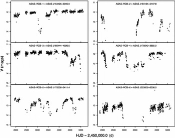
Figure 7. All Sky Automated Survey (ASAS-3) light curves of likely merger products R Coronae Borealis Stars ASAS-RCB-1 to ASAS-RCB-6 showing their characteristic, dramatic, and random dust obscuration events (Section 6.1). It is not known what the relationship between the merger history and the dust production properties are. Credit: image adapted from Figure 6 of Tisserand et al. (Reference Tisserand, Clayton, Welch, Pilecki, Wyrzykowski and Kilkenny2013).
The prevalence of close binaries amongst massive stars (Kiminki & Kobulnicky, Reference Kiminki and Kobulnicky2012; Sana et al., Reference Sana2012a, Section 2.1) leads us to the inevitable conclusion that many will interact and merge (de Mink et al., Reference de Mink, Sana, Langer, Izzard and Schneider2014). Should a sample of O stars be selected for single stars, as is typical in constructing observing surveys, up to half of these stars are likely to have once been binaries. If they have undergone mass transfer, their stellar structure, internal rotation profile, and nucleosynthetic history are likely to be quite different to a single star of equivalent mass. The number of these objects can be constrained by direct comparison with stellar clusters (Schneider et al., Reference Schneider2014), and modern binary population synthesis models agree remarkably well with observed main-sequence stellar mass functions if binaries are included. The most massive stars, such as the ~ 320 M⊙ R136a1 (Crowther et al., Reference Crowther, Schnurr, Hirschi, Yusof, Parker, Goodwin and Kassim2010), are also quite likely to be binary star mergers (Schneider et al., Reference Schneider2014). This said, a recent investigation of the R136a cluster by Crowther et al. (Reference Crowther2016) favours a scenario where not all very massive star are merger products, leaving open the question of how to form such stellar monsters.
6.2. Polluted white dwarfs
The class of WDs known as DZ includes stars with prominent metal lines in their spectra (van Maanen, Reference van Maanen1917; Weidemann, Reference Weidemann1960). The timescales for settling of metals in the atmospheres of WDs is short compared to the cooling time of the WDs. In many of these objects, it is therefore difficult to explain the presence of metals above the photosphere. Between a quarter and half of all WDs exhibit some degree of pollution (Zuckerman et al., Reference Zuckerman, Koester, Reid and Hünsch2003, Reference Zuckerman, Melis, Klein, Koester and Jura2010; Barstow et al., Reference Barstow, Barstow, Casewell, Holberg and Hubeny2014; Koester, Gänsicke, & Farihi, Reference Koester, Gänsicke and Farihi2014). The hottest WDs (T ≳ 20 000 K) can achieve metal levitation (Chayer, Fontaine, & Wesemael, Reference Chayer, Fontaine and Wesemael1995; Chayer, Reference Chayer2014; Koester et al., Reference Koester, Gänsicke and Farihi2014), but the cooler WDs must have recently accreted the metals (Koester, Reference Koester2009). Early explanations of the pollution phenomenon included accretion from the interstellar medium (Aannestad & Sion, Reference Aannestad and Sion1985; Sion, Aannestad, & Kenyon, Reference Sion, Aannestad and Kenyon1988), but it was not clear why some of the DZ WDs have helium atmospheres, because gas accreted from the interstellar medium would be mostly hydrogen.
Zuckerman & Becklin (Reference Zuckerman and Becklin1987) interpreted G29-38, a WD with a prominent infrared excess, as having a brown dwarf companion. Later, a certain number of DZ WDs were discovered to have similar infrared excess flux and a better interpretation was that these WDs were instead surrounded by small dusty disks, inside their Roche limits.
Alcock, Fristrom, & Siegelman (Reference Alcock, Fristrom and Siegelman1986) was the first to make the connection between the polluted WDs and the accretion of an asteroid or comet onto the WD. The arrival of an asteroid or comet at the Roche limit of the WD would result in it being pulverised, making a disk that would be visible at infrared wavelengths. Material from the disk is then accreted onto the surface of the WD, polluting the star. To date, approximately 30 such disks have been discovered, constituting approximately 1–3% per cent of the studied WDs (Farihi, Jura, & Zuckerman, Reference Farihi, Jura and Zuckerman2009). Occasionally, such WD debris disks are accompanied by a gaseous component, as is the case, for example, in SDSS J0845+2257 (Wilson et al., Reference Wilson, Gänsicke, Koester, Toloza, Pala, Breedt and Parsons2015).
Abundance analyses of DZ WD surfaces (e.g., Dufour et al., Reference Dufour, Kilic, Fontaine, Bergeron, Melis and Bochanski2012; Xu et al., Reference Xu, Jura, Koester, Klein and Zuckerman2014; Wilson et al., Reference Wilson, Gänsicke, Koester, Toloza, Pala, Breedt and Parsons2015) concluded that the observed elemental abundance distribution is similar to that of an asteroid with the average abundance of bulk Earth material (Figure 8). Subsequent analyses claimed to have detected patterns produced by asteroids of different compositions, such as those that have differentiated, or by water-carrying asteroids (in GD 61; Farihi et al., Reference Farihi, Gänsicke and Koester2013).

Figure 8. Compilation by Xu et al. (Reference Xu, Jura, Koester, Klein and Zuckerman2014) of all polluted white dwarfs (Section 6.2) with measured abundances for O, Mg, Si, and Fe. The abundances are always the dominant elements in a variety of extrasolar planetesimals, resembling bulk Earth. The abscissa marks white dwarf effective temperature, the ordinate their surface gravity. The size of each pie correlates with the accretion rate. Hydrogen-dominated white dwarfs: 1: G29-38 (Xu et al., Reference Xu, Jura, Koester, Klein and Zuckerman2014), 7: PG 1015+161, 8: WD 1226+110, 9: WD 1929+012, 10: WD 0843+516 (Gänsicke et al., Reference Gänsicke, Koester, Farihi, Girven, Parsons and Breedt2012); helium-dominated white dwarfs: 2: WD J0738+1835 (Dufour et al., Reference Dufour, Kilic, Fontaine, Bergeron, Melis and Bochanski2012), 3: HS 2253+8023 (Klein et al., Reference Klein, Jura, Koester and Zuckerman2011), 4: G241-6, 5: GD 40 (Jura et al., Reference Jura, Xu, Klein, Koester and Zuckerman2012), 6: GD 61 (Farihi et al., Reference Farihi, Brinkworth, Gänsicke, Marsh, Girven, Hoard, Klein and Koester2011; Farihi, Gänsicke, & Koester, Reference Farihi, Gänsicke and Koester2013). All white dwarfs except 3 and 4 have a dust disk. Bulk Earth: Allègre, Manhès, & Lewin (Reference Allègre, Manhès and Lewin2001). Comet Halley: Jessberger, Christoforidis, & Kissel (Reference Jessberger, Christoforidis and Kissel1988). Credit: figure adapted from Figure 18 of Xu et al. (Reference Xu, Jura, Koester, Klein and Zuckerman2014).
Questions do arise as to why the metal abundance patterns in some DZ WDs cannot always be explained by accretion, as is the case, for example, for SDSS J0845+2257, where the carbon abundance is too high to derive from accreted bodies and may be indigenous to the WD (Wilson et al., Reference Wilson, Gänsicke, Koester, Toloza, Pala, Breedt and Parsons2015).
The central star of planetary nebula NGC 6543, the Helix, has a 24-μm excess caused by the presence of a disk which could derive from disrupted Kuiper belt objects (Su et al., Reference Su2004). This disk may also be a left over from processes that took place during the AGB, as is likely the case for other central stars of PNe (Clayton et al., Reference Clayton, De Marco, Nordhaus, Green, Rauch, Werner and Chu2014) and post-AGB stars (Van Winckel et al., Reference Van Winckel2009).
The DZ WDs can therefore best be explained if they interacted with an asteroid, implying that 20–30% of all WDs have preserved parts of their planetary systems. This not only indicates that asteroid families commonly survive stellar evolution, but that an undetected, perturbing planet must exist at large distances from WDs in many cases.
6.3. The origin of non-spherical planetary nebulae and the unexplained bright edge of the planetary nebula luminosity function
The debate over what generates non-spherical PNe continues (De Marco, Reference De Marco2009; Kwitter et al., Reference Kwitter2014). On the theoretical front, there is still no viable quantitative theory to explain how single stars form highly non-spherical PNe, although there could be ways to form mildly elliptical shapes (e.g., Soker & Clayton, Reference Soker and Clayton1999). Single stars cannot sustain the interplay of rotation and magnetic fields that can alter the geometry of the AGB super-wind from a spherical, or almost spherical distribution (Soker, Reference Soker2006; Nordhaus et al., Reference Nordhaus, Blackman and Frank2007; García-Segura et al., Reference García-Segura, Villaver, Langer, Yoon and Manchado2014). Naturally, only a small fraction of PN can derive from interacting binaries because only a small fraction of binary systems has the appropriate orbital period to interact on the AGB (Section 2.2). Yet, 80% of all PN are non-spherical (Parker et al., Reference Parker2006), only some of which could be explained at the moment by single stars.
Alongside this problem, there is a host of additional key observations, which any comprehensive theory of PN formation must be able to explain:
-
(1) At least 15–20% of PNe have post-CE central stars (Section 4.2.2) in their centres, detected by light variability due to irradiation, ellipsoidal effects or eclipses in the close binaries (see Figure 9 and Section 3; Bond, Reference Bond, Kastner, Soker and Rappaport2000; Miszalski et al., Reference Miszalski, Acker, Moffat, Parker and Udalski2009a). These derive from those close main sequence binaries with progenitor primary masses between 1 and 2 M⊙, companion masses ≲1 M⊙, with an orbital separation shorter than 2–3 times the maximum AGB stellar radius of the primary of about 600 R⊙(Villaver & Livio, Reference Villaver and Livio2009; Mustill & Villaver, Reference Mustill and Villaver2012; Madappatt et al., Reference Madappatt, De Marco and Villaver2016). The expected fraction of post-CE central strs of PN is of the order of 5–10% (Han et al. Reference Han, Podsiadlowski and Eggleton1995; Nie, Wood, & Nicholls Reference Nie, Wood and Nicholls2012; Madappatt et al. Reference Madappatt, De Marco and Villaver2016) lower than the lower limit imposed by observations. This is not explained by current theory.
-
(2) Post-CE binary central stars are preferentially found inside bipolar nebulae, although some post-CE central stars are in elliptical PN (De Marco, Reference De Marco2009; Miszalski et al., Reference Miszalski, Acker, Parker and Moffat2009b; Hillwig et al., Reference Hillwig, Jones, De Marco, Bond, Margheim and Frew2016a), often with jets (Figure 10). The scale heights of spherical and bipolar PN are quite different (130 vs. 325 pc; Corradi & Schwarz Reference Corradi and Schwarz1995), which points to a larger progenitor mass in bipolars. There is also an association of bipolar PN with those of type I (N/O > 0.8; Kingsburgh & Barlow Reference Kingsburgh and Barlow1994), which must derive from progenitors with a mass larger than 3–5 M⊙ (Karakas et al., Reference Karakas, van Raai, Lugaro, Sterling and Dinerstein2009). Only stars with initial mass larger than 5 M⊙ can make type I PN. However, there could be mixing processes that allow stars with initial mass as low as 3 M⊙ to develop type I abundances. It is hard to reconcile the relatively large percentage of type I PN (~ 20%; Kingsburgh & Barlow Reference Kingsburgh and Barlow1994), with the initial mass function, that indicates that the fraction of stars more massive than 3 M⊙ is of the order of few per cent. It is even harder to understand the association of post-CE PN with a more massive population, although Soker (Reference Soker1998a) noted that the fact that more massive main sequence stars have binary companions more often (Section 2), and that they grow to larger radii, would promote a correlation between type I PN, post-CE PN, and bipolarity.
-
(3) Nie et al. (Reference Nie, Wood and Nicholls2012) used a binary population synthesis model calibrated to the fraction of giant stars that exhibit the sequence E phenomenon (Section 3.1), to predict how many PNe derive from a binary interaction. They concluded that 49–74% of PNe come from non-interacting binaries and single stars. However, they also predicted a fraction of single central stars in the range 3–19%, which cannot be reconciled with the much larger multiplicity fraction of the progenitor population (50 ± 4% for Solar-type stars; M MS = 1 − 1.3M⊙; Raghavan et al. Reference Raghavan2010, Section 2.1). A way to reconcile these numbers with data from main-sequence stars is to assume that not all 1–8 M⊙ stars make a visible PN. If AGB stars that interact with a companion made a brighter PN, then the detected fraction of post-interaction PN would be inflated.
-
(4) The bright edge of the PN luminosity function is almost invariant and, if one allows for small metallicity-dependent corrections, it predicts the distance to external galaxies with excellent precision for both old ellipticals and young spiral galaxies (Ciardullo, Reference Ciardullo2010). This indicates a ubiquitous population of relatively massive central stars in all galaxies. This disagrees with the prediction that PN in old elliptical galaxies have lower mass central stars. Ciardullo et al. (Reference Ciardullo, Sigurdsson, Feldmeier and Jacoby2005) argued that the data is consistent with PN from blue straggler stars (Section 3.3) populating the bright end of the luminosity function.

Figure 9. Observed V, R, and I phase-folded light curves of the post-common envelope central binary star of planetary nebula HaTr 4 for a period of 1.74 days. The variability is due to a combination of irradiation of the main sequence companion by the hot central star as well as eclipses. Such close binaries comprise at least 15 per cent of all central stars of planetary nebula. The solid and dashed lines correspond to two models using a Wilson-Devinney code using different parameter sets, as described in Hillwig et al. (Reference Hillwig, Bond, Frew, Schaub and Bodman2016b). Credit: image adapted from Figure 1 of Hillwig et al. (Reference Hillwig, Bond, Frew, Schaub and Bodman2016b)

Figure 10. The planetary nebula Fleming 1, with its prominent jets, was ejected during a common envelope (Section 4.2.2) interaction between an AGB star and its companion. The core of the AGB star and the companion are today at the core of the nebula (Section 6.3). Credit: image from Figure 2 of Boffin et al. (Reference Boffin, Miszalski, Rauch, Jones, Corradi, Napiwotzki, Day-Jones and Köppen2012).
6.4. The effects of binary interaction on the population of Wolf–Rayet stars and luminous blue variables
The fact that about 70% of massive stars interact with a companion (Section 2) reinforced the suspicion that previously known massive star phenomena may have a binary origin, at least in a fraction of the objects. Here, we concentrate in particular on the WR phenomenon (Section 6.4.1), luminous blue variables (LBVs; Section 6.4.2), and core collapse supernovae (see also Section 6.5).
6.4.1. Wolf–Rayet stars
WR stars (Wolf & Rayet, Reference Wolf and Rayet1867) are rare, luminous stars with strong emission lines, occasionally with P-Cygni profiles of helium, nitrogen, carbon, and oxygen indicating strong, mass-losing winds. WR stars dominated by nitrogen lines are called ‘WN’. The ‘WC’ and ‘WO’ types have emission lines of, predominantly, carbon and oxygen, respectively. It is thought that they form a sequence in that the earlier phase, the WN, gives rise to the later phase, WC/O once the strong winds have eliminated the nitrogen-rich layer (for a review, see Crowther, Reference Crowther2007).
The winds of WR stars are line-driven as was discovered once UV-spectroscopy of massive stars became available (Morton, Reference Morton1967). The original explanation of this rare phenomenon leaned towards a binary interpretation, where the companion strips the mass off the massive star by Roche-lobe overflow (e.g., Paczyński, Reference Paczyński1966). However, the realisation that WR stars have high-mass loss rates, up to 10−4 M⊙ yr, as well as a series of population studies that reconciled the relative numbers of O and WR stars (Massey, Reference Massey2003), provided a reasonable, single-star explanation for the WR phenomenon. Later, the understanding that WR winds are clumped lead to a downward revision of the mass-loss rates deduced from UV and optical observations (Vink & de Koter, Reference Vink and de Koter2005) and, once again, the interpretation of the WR phenomenon included, at least in part, the effects of binary interactions.
There are several cases in which a WR star is known to have a binary companion. The binary fraction in the massive WR population is 40% both in the Galaxy and in other populations such as the Small Magellanic Cloud (Foellmi, Moffat, & Guerrero, Reference Foellmi, Moffat and Guerrero2003). This is somewhat contrary to the expectation that a lower metallicity would reduce stellar wind mass loss rates and leave only binary interactions to strip stars of their hydrogen, something that would have driven the Small Magellanic Cloud WR binary fraction up. It is also expected that in a binary, even lower mass stars may develop the WR phenomenon. However, Shenar et al. (Reference Shenar2016) found that in the Small Magellanic Cloud WR binaries have masses in excess of the limit above which single stars should be capable of entering a WR phase at those metallicities. Clearly, mass-loss has a large impact on the evolution of the star and its observed quantities, but just what the interplay of binarity and mass-loss is on the WR phenomenon remains at this time hard to pinpoint.
Langer (Reference Langer2012) argues that (1) the detected population of WR stars is not particularly impacted by binary interactions, in other words we can be reasonably sure that the current WR stars are not the product of mergers and (2) that there is a large population of low-mass, low luminosity WR stars that is thus far undetected. Their progenitors are massive Algols where the donor can be an O or at most an Of/WN star (Rauw, Vreux, & Bohannan, Reference Rauw, Vreux and Bohannan1999). The donor will likely develop into a WR star when it loses more mass to the companion in what Langer (Reference Langer2012) calls Case AB mass transfer. Their progeny would be the Be/X-ray binaries (Liu et al., Reference Liu, van Paradijs and van den Heuvel2006).
Aside from WR stars in short-period binaries (e.g., SMC AB6, with a 6.5 d period; Shenar et al. Reference Shenar2016), some WR binaries have periods from tens to hundreds of days and some are found to have colliding winds, as observed in X-ray light curves (e.g., WR21a; Gosset & Nazé Reference Gosset and Nazé2016). Occasionally, dust forms in the wake of these collisions and the WR can be observed as a pinwheel nebula such as WR104, discovered by Tuthill, Monnier, & Danchi (Reference Tuthill, Monnier and Danchi1999). Since the prototype, several other similar pinwheel nebulae have been discovered, such as WR98a (Monnier, Tuthill, & Danchi Reference Monnier, Tuthill and Danchi1999), as well as two in the Quintuplet star cluster (Tuthill et al., Reference Tuthill, Monnier, Tanner, Figer, Ghez and Danchi2006). This cluster is one of the most massive in our Galaxy and is named after the five mysterious red sources with very high luminosity, which have been interpreted both as young and evolved stars (Okuda et al., Reference Okuda1990). All five sources were resolved by the Keck telescope using speckle interferometry (Tuthill et al., Reference Tuthill, Monnier, Tanner, Figer, Ghez and Danchi2006) and two of these sources, with the largest sizes, are superimposed on a Hubble Space Telescope image of the cluster in Figure 11.
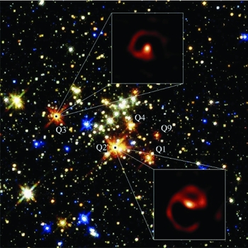
Figure 11. Multiwavelength Hubble Space Telescope, Near Infrared Camera and Multi Object Spectrograph near-infrared image of the Quintuplet cluster (for details of the image, see Figer, McLean, & Morris Reference Figer, McLean and Morris1999). The five red stars are labelled according to the nomenclature of Moneti, Glass, & Moorwood (Reference Moneti, Glass and Moorwood1994). All of them are ‘dustars’, dust-producing, binary Wolf–Rayet stars (Section 6.4.1). Inset images of Q2 and Q3 recovered with Keck telescope speckle interferometry are overlaid, with graphical indication showing the relative scaling between the Hubble and Keck images. Credit: image adapted from Figure S1 of Tuthill et al. (Reference Tuthill, Monnier, Tanner, Figer, Ghez and Danchi2006).
It is likely that a number of other WR stars with dust implied by high IR fluxes or with colliding winds implied by non-thermal radio emission (for example, WR104, WR98a, as well as WR48a WR112 and WR140; for a summary, see Monnier et al. Reference Monnier, Tuthill, Danchi, Murphy and Harries2007) may be such pinwheels but either too far or at a non-favourable inclination to be resolved (e.g., WR112; Monnier et al. Reference Monnier, Tuthill, Danchi, Murphy and Harries2007). Whilst these binaries may be too wide for violent phenomena to occur, an important aspect of their geometry is that their wind–wind collision zones seem to promote the manufacture of carbon dust, despite the hot environment, sometimes at rates as high as 10−6 M⊙ yr−1 (Williams, Reference Williams1995). It is not known how many dust-making WR stars (dustars) exist in the Galaxy today, but numbers such as 100–1 000 are not unlikely based on new surveys (Shara et al., Reference Shara2009, Reference Shara, Faherty, Zurek, Moffat, Gerke, Doyon, Artigau and Drissen2012) that are finding large numbers of the cooler, WC9 type WR stars near the Galactic centre. If this were the case, this type of WR binary would produce dust at rates commensurate to the classic dust producers, such as red supergiants, AGB stars, PNe, and supernovae (Marchenko & Moffat, Reference Marchenko, Moffat, St.-Louis and Moffat2007; Draine, Reference Draine, Henning, Grün and Steinacker2009).
6.4.2. Luminous blue variables
LBVs have for a long time been interpreted as massive stars at the transition between the end of hydrogen burning and the start of core helium burning that undergo eruptive phases of mass loss. In a scenario laid out first by Conti (Reference Conti1978), O stars go through strong mass-loss rates turning them into WR stars of class WNH (Smith & Conti, Reference Smith and Conti2008), before an LBV eruption frees them of all hydrogen and turns them into WC/WO WR stars and eventually type Ib and Ic supernovae (e.g., Crowther et al., Reference Crowther2000). At first, it was thought that the main mechanism by which LBVs shed large amounts of mass would be line-driven winds (Humphreys & Davidson, Reference Humphreys and Davidson1994; Lamers & Nugis, Reference Lamers and Nugis2002). In this scenario, the LBV outburst is due to an increase in the bolometric luminosity together with a decrease of the mass via mass loss, which leads to a high ratio of luminosity to mass, which in turn brings the star close to the Eddington limit. However, Smith & Owocki (Reference Smith and Owocki2006) showed that a more likely mechanism is a super-Eddington wind driven by continuum radiation pressure.
Several problems affect the standard LBV scenario and the evolution of massive stars in general. The LBV S Doradus had an outburst with a measured mass-loss rate far below that needed to explain the expanding pseudo-photosphere envisaged by classical LBV theory (de Koter, Lamers, & Schmutz, Reference de Koter, Lamers and Schmutz1996; Groh et al., Reference Groh, Hillier, Damineli, Whitelock, Marang and Rossi2009). Nor did the luminosity changes observed happen at constant bolometric luminosity (Groh et al., Reference Groh, Hillier, Damineli, Whitelock, Marang and Rossi2009). The brightness outburst in S Doradus seemed rather driven by a ‘pulsation’ of the envelope (Gräfener, Owocki, & Vink, Reference Gräfener, Owocki and Vink2012). Similarly, light echo spectra of the Great Eruption of η Carinae (Rest et al., Reference Rest2012) are inconsistent with a pseudo-photosphere and more in line with the spectra of transients NGC 4990-OT and V 838 Mon (Smith et al., Reference Smith2016b, see also Section 7.2), that are suspected binary mergers.
Further problems arise because the most likely progenitors of some type IIn supernovae (hydrogen-rich supernovae with narrow lines) have LBV-like mass-loss rates and in four cases progenitors are known, e.g., SN 1961V (Smith et al., Reference Smith2011b; Kochanek, Szczygiel, & Stanek, Reference Kochanek, Szczygiel and Stanek2011), 2005gl (Gal-Yam & Leonard, Reference Gal-Yam and Leonard2009), 2010jl (Smith et al., Reference Smith2011b), and 2009ip (Smith et al. Reference Smith2010, Foley et al. Reference Foley, Berger, Fox, Levesque, Challis, Ivans, Rhoads and Soderberg2011; see also Smith (Reference Smith2014) for a review). However, in the Conti scenario, LBVs do not explode as type II supernovae, rather they spend 0.5–1 Myr as WR stars, which then explode as type Ib or Ic supernovae.
Approximately, a dozen (eruptive) LBVs are known in the Galaxy and Magellanic Clouds (e.g., Clark, Larionov, & Arkharov, Reference Clark, Larionov and Arkharov2005) with another dozen known in external galaxies. Smith & Tombleson (Reference Smith and Tombleson2015) found that LBV stars are statistically more isolated than O and WR stars in the Galaxy and in Large Magellanic Cloud clusters, indicating that LBVs cannot in all cases be a phase in the evolution of O and WR stars. They proposed alternative binary scenarios for at least a fraction of the objects.
It was Gallagher (Reference Gallagher, Davidson, Moffat and Lamers1989) who first discussed the LBV phenomenon in connection with binary stars. Many papers discuss the famous η Carinae eruptions (Figure 12) arguing for and against a binary interpretation. A B-type companion was announced in 2005 (Iping et al., Reference Iping, Sonneborn, Gull, Massa and Hillier2005, see also Soker Reference Soker2001 and references therein), but it later transpired that the observations that were interpreted as a companion detection could have been explained by alternative effects (e.g., Martin et al., Reference Martin, Davidson, Humphreys, Hillier and Ishibashi2006). The 5.5-yr spectroscopic cycle (e.g., Zanella, Wolf, & Stahl, Reference Zanella, Wolf and Stahl1984) of emission lines periodically increasing in strength, also seen as an X-ray brightening (Ishibashi et al., Reference Ishibashi, Corcoran, Davidson, Swank, Petre, Drake, Damineli and White1999), tends to be explained as a companion in an eccentric orbit where the X-ray luminosity increases near periastron due to colliding winds and the spectroscopic event is due to mass ejection at periastron (e.g., Mehner et al., Reference Mehner, Davidson, Ferland and Humphreys2010). However, a direct detection of the companion is yet to be accomplished.

Figure 12. Hubble Space Telescope, Wide Field, and Planetary Camera 2 images of gas ejected during the Great Eruption of the luminous blue variable η Carinae (Section 6.4.2). False colour in five optical bands. The image is approximately 40 arcsec on a side. North is towards the bottom left corner, east is towards the bottom right corner. Credit: image courtesy of the Hubble Site, associated with press release STScI-2009-25.
Iben (Reference Iben, Morse, Humphreys and Damineli1999) suggested that the Great Eruption of η Carine was due to a merger in a triple system, but it is difficult to understand further eruptions in the same system. Soker (Reference Soker2004b) envisaged how the Great Eruption could be interpreted as a binary interaction at the time of periastron and even extended this interpretation to some ‘supernova impostors’ (see Section 7.2.1). Accretion at periastron passage would power jets that eventually form the Homunculus, the bi-polar structure that is so well known today (Figure 12).
However, some aspects of this presumed interaction are inconsistent with observations (Smith, Reference Smith2011). In particular, one question is the distance of the periastron passage compared to the photospheric radius and the Roche lobe of the primary. Staff et al. (Reference Staff, De Marco, Macdonald, Galaviz, Passy, Iaconi and Low2016a) showed that any mass transfer between the primary and the secondary at periastron passage shortens the period of the binary leading eventually to a CE phase and possibly a merger. This would mean that the 5.5 yr orbit would not be stable as is instead observed.
It is likely that there are multiple classes of LBVs and that the proximity of a companion plays a major role in many LBVs, particularly when the stellar mass is too low to exhibit single-star instabilities. Ultimately, just the range of parameters that drive binary evolution compared to those that regulate a single star, would help expain a broad range of behaviours, such that identifying specific classes is difficult. In Sections 6.5 and 7, we discuss the related phenomena of supernovae and supernova impostors, emphasising how upcoming transient surveys will give us a sufficient number of objects to start identifying broad behavioural classes.
6.5. Hydrogen-deficient, type I supernovae
Supernovae of type I are explosions, presumably of stars, that show no evidence for hydrogen in their spectra. These can be subdivided into the silicon-rich Ia, and types Ib and Ic, which have no, or weak silicon lines in their spectra, but have helium (Ib) or do not (Ic). The modern consensus is that the type Ia supernovae are thermal runaway explosions of carbon–oxygen WD (e.g., Hillebrandt & Niemeyer, Reference Hillebrandt and Niemeyer2000), whilst Ib and Ic supernovae are helium stars that undergo core collapse (e.g., Smartt, Reference Smartt2009). The mechanisms for explosion are quite different, but binary stars are related to both.
6.5.1. Type Ia supernovae
Type Ia supernovae are famous for having provided the standard candles required by cosmologists to deduce that the Universe is expanding (Leibundgut, Reference Leibundgut2001). They are not true standard candles, rather they are standardisable, meaning that their maximum brightness correlates with the width of their lightcurves (Phillips, Reference Phillips1993), at least in local type Ia supernovae. Thus, given their lightcurve width, their intrinsic brightness can be calculated, and hence their distance.
Despite their successful use as cosmological tools, we do not know for sure what causes a type Ia supernova. The most likely scenario is that type Ia supernovae are exploding carbon–oxygen WD with masses near the Chandrasekhar mass limit of about 1.4M⊙ (Wang & Han, Reference Wang and Han2012). WDs are no longer undergoing nuclear fusion and their gravitational collapse is resisted by electron degeneracy pressure. If such a WD accretes mass in a binary star system, the central density and temperature increase and, eventually, core carbon ignites. The degenerate nature of the star leads to a thermonuclear runaway and to the disruption of the entire star. It is necessary to invoke CE interactions (Section 4.2.2) to make stellar systems containing a carbon–oxygen WD in a suitably short orbit for any mass transfer to occur.
There are many outstanding theoretical problems related to type Ia supernovae. The details of the explosion matter greatly to the nucleosynthetic signature of its remnant. Whether the explosion is a subsonic deflagration, a supersonic detonation or some combination of the two is unclear at present. There are successful 2D and 3D models of type Ia supernovae (e.g. Fink et al. Reference Fink2014), although the explosion triggering is still largely based on simplified physics.
The total number of systems which explode as type Ia supernovae can be predicted by binary population synthesis models (Section 4.2.3). Whilst there are many uncertainties involved, not least the problem of CE evolution described above, estimates between different research groups are remarkably consistent (Toonen et al., Reference Toonen, Claeys, Mennekens and Ruiter2014). However, these theoretical estimates are a factor of 4 to 10 lower than observational rates (Claeys et al., Reference Claeys, Pols, Izzard, Vink and Verbunt2014). The problem is that we just do not know which stars explode as type Ia supernovae, or how their progenitor systems form in the first place. Double degenerate systems contain two WDs (Nelemans et al., Reference Nelemans2005) which, if they can merge to form a single WD in excess of the ignition mass, may explode. Such systems are observed, but it remains a great challenge to model their formation. Maybe triple systems offer a solution in some cases, increasing the rate of merging, but it is not clear that there are enough systems in the appropriate parameter space to match the observed type Ia supernova rate (Hamers et al., Reference Hamers, Pols, Claeys and Nelemans2013).
Single-degenerate systems remain candidates for type Ia supernova progenitors, but the evidence is mixed. They involve mass transfer from a giant or sub-giant star to a WD, which increases its mass beyond the limit for ignition. No type Ia supernova contains hydrogen, which would be expected from the majority of donor stars, thus putting this model in doubt or at least rendering it rare. An alternative is helium donors, which are likely significant (Claeys et al., Reference Claeys, Pols, Izzard, Vink and Verbunt2014). This said, despite repeated searches for companions, some of which imposed stringent limits on their absence (Schaefer & Pagnotta, Reference Schaefer and Pagnotta2012), strong evidence for a main-sequence companion was recently presented by Marion et al. (Reference Marion2016) and a UV signature detected by the Swift Telescope 4d after the explosion is consistent with supernova ejecta impacting a companion star in the case of iPTF14atg (Cao et al., Reference Cao2015).
A comparison of different scenarios that may lead to a type Ia supernova explosion can be found in Tsebrenko & Soker (Reference Tsebrenko and Soker2015) who also discuss the fraction of type Ia supernovae that may occur inside of a planetary nebula.
6.5.2. Type Ib,c supernovae
Type Ib and Ic supernovae are thought to be explosions caused by the collapsing cores of stars that have lost their hydrogen (Ib) and helium (Ic) envelopes. Because a massive star must lose much of its mass to expose its helium or carbon–oxygen core, binaries are naturally invoked as a cause (Podsiadlowski et al., Reference Podsiadlowski, Joss and Hsu1992; Eldridge et al., Reference Eldridge, Izzard and Tout2008). However, stellar wind mass loss is significant even in single massive stars (Vink, de Koter, & Lamers, Reference Vink, de Koter and Lamers2001) and, perhaps combined with rotation, is sufficient to lead to type Ib and Ic supernovae. The formation of progenitor systems of type Ib and Ic supernovae, the WR stars, can probably form by both wind mass loss and rotational mixing in rapidly spinning single stars (Yoon & Langer, Reference Yoon and Langer2005) as well as binary interactions.
Helium stars with masses in excess of 5 M⊙ should have been seen by various supernova progenitor search programmes, but they have not. This may imply that massive helium stars do not explode as supernovae, instead they collapse directly to black holes. Lower-mass helium stars are even more likely to form by of binary interactions because wind mass loss is weaker at lower luminosities and hence lower mass. Searches for progenitors may simply not be sensitive enough to see low-mass helium star progenitors of distant supernovae (Yoon et al., Reference Yoon, Gräfener, Vink, Kozyreva and Izzard2012).
Eldridge et al. (Reference Eldridge, Fraser, Smartt, Maund and Crockett2013) presented an extensive search for the progenitors of type Ib and Ic supernovae in all available pre-discovery imaging since 1998, finding that 12 type Ib and Ic supernovae have no detections of progenitors in either deep ground-based or Hubble Space Telescope imaging. They showed that the deepest absolute B, V, and R-band magnitude limits are between − 4 and − 5. By comparing these limits with the observed WR population in the Large Magellanic Cloud, they estimated statistically that a failure to detect such a progenitors by chance is unlikely. They proposed an alternative that the progenitors of type Ib and Ic supernovae evolve significantly before core-collapse.
Eldridge et al. (Reference Eldridge, Fraser, Smartt, Maund and Crockett2013) also reviewed the relative rates and ejecta mass estimates from light-curve modelling of type Ib and Ic supernovae, and found both data sets incompatible with WR stars with initial masses > 25 M⊙ being the only progenitors. Finally, they presented binary evolution models that fit the observational constraints and determined that stars in binaries with initial masses ≲ 20 M⊙ lose their hydrogen envelopes in binary interactions to become low-mass helium stars. They retain a low-mass hydrogen envelope until ~ 10−4 yr before core-collapse, so it is not surprising that Galactic analogues have been difficult to identify. The predictions of Eldridge et al. (Reference Eldridge, Fraser, Smartt, Maund and Crockett2013) may have been bourn out in the discovery of a possible progenitor of SN iPTF13bvn (Cao et al., Reference Cao2013) that is consistent with a lower mass helium star, but inconsistent with a WR progenitor (Eldridge et al., Reference Eldridge, Fraser, Maund and Smartt2015).
Crowther (Reference Crowther2013) concluded that supernovae type Ib and Ic are more frequently associated with HII regions than type II supernovae, pointing to a larger progenitor mass, though he could not differentiate between type Ib and Ic. Anderson et al. (Reference Anderson, James, Habergham, Galbany and Kuncarayakti2015) showed that type Ic are more often associated with Hα emitting galaxies than type Ib, pointing to a higher progenitor mass for that type. This conclusion is also in line with the study of Smith et al. (Reference Smith, Li, Silverman, Ganeshalingam and Filippenko2011c), who advocated a mixed origin for the supernovae type Ib and Ic, with single stars able to produce some supernovae type Ic, which would then have a higher progenitor mass. Additionally, single stellar evolution predicts an increase in the ratio of supernova type Ib and Ic to supernova type II with increasing metallicity, due to higher mass-loss rates at higher metallicity (e.g., Heger et al., Reference Heger, Fryer, Woosley, Langer and Hartmann2003; Ibeling & Heger, Reference Ibeling and Heger2013). However, an increase of the ratio with oxygen abundance, used as proxy for metallicity, was not observed by Anderson et al. (Reference Anderson, James, Habergham, Galbany and Kuncarayakti2015, Figure 13), except for the lowest metallicity bin, where a lower ratio was reported.

Figure 13. The ratio of supernovae type Ib and Ic to supernovae type II as a function of metallicity, measured from the oxygen abundance in HII regions. The lack of a decrease in this ratio with increasing metallicity argues for a mixed origin for these type of supernovae (Section 6.5.1). Credit: image adapted from Figure 10 of Anderson et al. (Reference Anderson, James, Habergham, Galbany and Kuncarayakti2015).
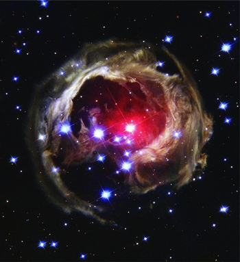
Figure 14. Hubble Space Telescope image of the gap transient V 838 Mon, taken on February 8, 2004 (Section 7.2.3). This gap transient is thought to be due to a merger of two stars. The dust illuminated by the outburst is not ejected by the object but has an interstellar origin. Composite image constructed using three filters: F435W (B), F606E (V), F814W (I). North is towards the top-left of the image. The image is 2.4 arcmin across or 4.2 parsec at a distance of 6 pc. Credit: Hubble Space Telescope program 10089, PI Noll.
In conclusion, there is little doubt that binary stellar evolutionary channels account for a substantial fraction and for the diversity of supernova types, though the interplay of single and binary evolutionary channels is likely to increase the complexity of the supernova phenomenon.
7 TRANSIENTS
Transients related to binary stellar evolution are either outbursts, or other periodic or semi-periodic light changes. Well-known transients include cataclysmic variables such as novae and dwarf novae (Table 1), which are observed locally and are very numerous. Other, more rare transients are supernovae, which being more luminous can be observed out to much greater distances. Occasionally, a transient is observed that has an unknown nature. These tend to be studied intensely, e.g., V 838 Mon (Figure 14), with over 300 articles since 2002, but seldom form a new class because of their rarity.
7.1. Surveys for transients
Transient surveys have increased the number of known transients and generated a sufficient number of objects that new classes have been established. Even with modest size telescopes, they have revolutionised the field of transient studies and, because many transients are likely binary phenomena, the field of binaries itself. Even before the latest wave of transient surveys, which we detail below, supernova searches were detecting transients that do not squarely fall within the supernova classification. For example, the Lick Observatory Supernova Search (LOSS) using a 76-cm robotic telescope (Filippenko et al., Reference Filippenko, Li, Treffers, Modjaz, Paczynski, Chen and Lemme2001).
Examples of more modern dedicated surveys are the Catalina Real-Time Transient Survey (CRTS; Drake et al. Reference Drake2009), the Palomar Transient Factory (PTF; Law et al. Reference Law2009), Pan-STARRS1 (Kaiser et al., Reference Kaiser, Stepp, Gilmozzi and Hall2010), and SkyMapper (Murphy et al., Reference Murphy, Keller, Schmidt, Tisserand, Bessell, Francis, Costa, Murphy and Bessell2009). All these surveys are optical in nature and use 1-m-class and 2-m-class telescopes. In addition, surveys designed to detect near Earth objects (e.g., LINEAR, Stokes et al. Reference Stokes, Evans, Viggh, Shelly and Pearce2000) are also used to detect transients (Palaversa et al., Reference Palaversa, Gezari, Sesar, Stuart, Wozniak, Holl and Ivezić2016). There are also transient surveys using non-dedicated telescopes and instruments, usually targeting specific parameter spaces, such as high cadence surveys for fast transients (e.g., Subaru Hyper Suprime-Cam Survey Optimised for Optical Transients, SHOOT; Tanaka et al. Reference Tanaka2016, or the High Cadence Transient Survey, HiTS; Forster et al. Reference Forster, Maureira, Gonzalez-Gaitan and Galbany2014).
Upcoming surveys such as the Zwicky transient survey (Smith et al., Reference Smith, Ramsay, McLean and Takami2014), will survey 3 750 deg2 an hour, 15 times faster than its predecessor the PTF. Finally, the Large Synoptic Survey Telescope (LSST; Ivezic et al. Reference Ivezic2008), with an 8.4-m mirror and a plan to scan 30000 deg2 of sky every third night, should detect a huge number of phenomena, many of which are currently unknown. Most will be so faint that they will require follow up by high-demand telescopes such as the James Webb Space Telescope or a 30-m class telescope.
Other surveys take different strategies. The Public European Southern Observatory Spectroscopic Survey of Transient Objects (PESSTO; Smartt et al. Reference Smartt2015), follows up photometrically and spectroscopically specific transients selected from publicly available sources and wide-field surveys.
At wavelengths other than optical, X-ray transient surveys reveal a range of binary interaction activities, primarily in high-mass X-ray binaries with black hole (e.g., Tetarenko et al., Reference Tetarenko, Sivakoff, Heinke and Gladstone2016) or neutron star (e.g., Bozzo, Falanga, & Stella, Reference Bozzo, Falanga and Stella2008) accretors. The new SPitzer InfraRed Intensive Transients Survey (SPIRITS; Kasliwal et al. Reference Kasliwal2014) should detect year-long transients produced by slow in-spiral because of outflow from the second Lagrangian point (Pejcha, Metzger, & Tomida, Reference Pejcha, Metzger and Tomida2016). It can also detect dust formation in explosive events (e.g., in V 1309 Sco, Nicholls et al., Reference Nicholls2013) and find transient events that have no optical counterpart. A large number of radio transient surveys have been operational for a long time (e.g., Williams et al., Reference Williams, Bower, Croft, Keating, Law and Wright2013) but the new capabilities of the Australian Square Kilometre Array Pathfinder, ASKAP (e.g. the Variables and Slow Transient, VAST, survey) and eventually the Square Kilometre Array will add a new dimension to the searches (see, e.g., Metzger, Williams, & Berger, Reference Metzger, Williams and Berger2015).
If we add to these upcoming surveys, the new capability of gravitational wave detection (Section 7.4), we see how their combined power provides us with a new tool to study interacting binaries and connect scattered events into a coherent picture.
7.2. Gap transients
The luminosity gap between the faint and numerous novae and the bright but rarer supernovae is being increasingly filled. Such transients used to be discovered by amateur astronomers (e.g., SN2008S, Arbour & Boles Reference Arbour and Boles2008) or serendipitously, as is the case for M31 RV that erupted in 1988 (Rich et al., Reference Rich, Mould, Picard, Frogel and Davies1989). Such discoveries were only sporadically followed up. The proliferation of new surveys such as the CRTS and PTF has increased the number of gap transients detected.
We distinguish three types of gap transients following the nomenclature of Blagorodnova et al. (Reference Blagorodnova2016): Supernova impostors, thought to be non-terminal eruptions in massive stars such as LBVs; intermediate luminosity optical (or red) transients (ILOTs/ILRTs), explained as faint terminal explosions and luminous red novae (LRNs), which are potential stellar mergers. The terminology ILOT is, however, variably used to encompass all gap transients, for example, by Kashi & Soker (Reference Kashi and Soker2016), who also envisaged, but not without controversy (Smith et al., Reference Smith2011b), a more unified interpretation for the entire class. The division above is based on interpretation, rather than on observational characteristics. Whilst a classification system should stay away from interpretation, it is possible that at this time the observational qualities of these transients are still too disparate and the observations too uneven to lead to a proper classification.
7.2.1. Gap transients: supernova impostors
Searches for supernovae have discovered eruptive events thought to be similar to LBV eruptions, which are too rare to be readily observed in our Galaxy. These have been called supernova ‘impostors’. Supernova impostors are characterised by type IIn spectra with lower peak luminosities than typical core collapse supernovae (MV ~ −13 instead of ~ −17; Van Dyk et al. Reference Van Dyk, Peng, King, Filippenko, Treffers, Li and Richmond2000).
It has been realised in the past decade that there is quite a diversity amongst the supernova impostors. Whilst some have high luminosity and may derive from high mass stars, some may come from stars with lower mass progenitors (Prieto et al., Reference Prieto2008; Thompson et al., Reference Thompson, Prieto, Stanek, Kistler, Beacom and Kochanek2009) that should not approach the Eddington limit, raising the possibility of alternative pathways to these phenomena, possibly including a binary companion. Some supernova impostors, with sustained high luminosity phases could be powered by an ejection that ploughs into circumstellar material, transforming kinetic energy into luminosity. However, we do not yet have a model that produces the circumstellar shell in the first place.
Examples of the supernova impostor class are η Carinae, R127, and S Doradus (Walborn et al., Reference Walborn2008) in the Large Magellanic Cloud, SN 2009ip (Fraser et al., Reference Fraser2013) or UGT 2773 OT2009-1 (Smith et al., Reference Smith, Andrews, Mauerhan, Zheng, Filippenko, Graham and Milne2016a). These eruptions happen in dusty environments created by past outbursts. Some impostors have been, in turn, interpreted as massive binary stars. For example, the X-ray signature in supernova SN 2010da is consistent with it being a high-mass X-ray binary (Binder et al., Reference Binder, Williams, Kong, Gaetz, Plucinsky, Dalcanton and Weisz2011, Reference Binder, Williams, Kong, Gaetz, Plucinsky, Skillman and Dolphin2016). Some supernova impostors could be powered by repeated interaction in massive eccentric binaries (e.g., Kashi, Soker, & Moskovitz, Reference Kashi, Soker and Moskovitz2013).
7.2.2. Gap transients: intermediate luminosity optical, or red transients
ILOTs/ILRTs such as SN 2008S (Prieto et al., Reference Prieto2008), NGC 300 2009OT-1 (Bond et al., Reference Bond, Bedin, Bonanos, Humphreys, Monard, Prieto and Walter2009), or iPTF10fqs (Kasliwal et al., Reference Kasliwal, Cenko, Kulkarni, Ofek, Quimby and Rau2011) at the luminous end of the gap have been interpreted as faint terminal explosions, because of the complete disappearance of the progenitor after the outburst. They are associated with dusty environments and are tentatively hypothesised to derive from electron-capture supernovae (Botticella et al., Reference Botticella2009) after a short and dusty transition phase lasting approximately 10 000 yrs. Kashi & Soker (Reference Kashi and Soker2016) interpret ILRTs as less massive versions of supernova impostors and they argue that both groups are non-terminal outbursts due to mass accretion onto a companion in an eccentric orbit. As we already pointed out in Section 4.2.1, this rests on finding a suitable accretion model, which at the moment is beyond our understanding.
7.2.3. Gap transients: luminous red novae
LRNe are thought to be violent binary interactions (Iben & Tutukov, Reference Iben and Tutukov1992; Soker & Harpaz, Reference Soker and Harpaz2003). The best studied example is V1309 Sco (Tylenda et al., Reference Tylenda2011a, Figure 15), a system discovered serendipitously, but which is in the OGLE field of view hence has a long baseline of pre-outburst observations. V 1309 Sco is very likely be a merger because the light curve before the outburst showed a contact binary, and this binary disappeared after the outburst.

Figure 15. The I band light curve of the gap transient V1309 Sco I- from Tylenda et al. Reference Tylenda2011a, showing a slow rise in brightness over ~ 4 yrs prior to the outburst (Section 7.2.3). The range of brightness seen before the dip at JC24500004500 is due to variability caused by ellipsoidal distortion in the pre-outburst, contact binary. Due to the absence of the binary after the outburst, this is the best observational example of a merger we have to date. Credit: image from Tylenda et al. (Reference Tylenda2011a)
Another well studied example of an LRN is V 838 Mon (Bond et al., Reference Bond2003), which was followed by several similar outbursts (e.g., Williams et al., Reference Williams, Darnley, Bode and Steele2015). More massive objects can be seen out to larger distances and as such it is likely that these more rare phenomena will be those observed more often. An example of a massive transient that likely shared many characteristics with V 838 Mon is M101-OT (Blagorodnova et al., Reference Blagorodnova2016). This object peaked in brightness in 2014 and 2016. Archival photometry shows a binary system with a mass ratio of 0.9 and a total mass of 20 M⊙ that underwent a CE phase as the primary ended core hydrogen fusion. The mass of the progenitor fills the gap between the lower mass examples such as V 838 Mon (5–10 M⊙) and the more massive examples such as NGC 4490-OT (30 M⊙; Smith et al., Reference Smith2016b). A model of the scenario also predicts that the binary survived the CE phase.
Smith et al. (Reference Smith2016b) also point out that NGC 4490-OT fits the correlation between merger mass and peak luminosity discovered by Kochanek (Reference Kochanek2014, see Figure 16), adding a more massive, more luminous data point. They also show that there could be a correlation between mass, peak luminosity, and the duration of the outburst. Finally, they point out how the light echo spectrum of η Car (Rest et al., Reference Rest2012) is similar to the spectrum of NGC 4490-OT and that of V 838 Mon at some epoch, connecting LRNe and supernova impostors. They propose that η Car could be an even more massive example within the same correlation, having had a brighter and longer lasting outburst.

Figure 16. Absolute magnitudes of the progenitors (open symbols) and transient peaks (filled symbols) in the V (squares) and I (triangles) bands, as a function of the progenitor mass estimates for gap transients (Section 7.2). The best power-law fits are also shown. Credit: adapted from Figure 5 of Kochanek (Reference Kochanek2014).
7.2.4. Gap transients: sundry
Other gap transients not fitting well within the characteristics of the previous classes are the. Ia supernovae, first conjectured by Bildsten et al. (Reference Bildsten, Shen, Weinberg and Nelemans2007, see also Shen et al. Reference Shen, Kasen, Weinberg, Bildsten and Scannapieco2010) to be surface detonations on CO WDs following accretion from a less massive, companion WD. The best case of such a supernova detected to date was described by Kasliwal et al. (Reference Kasliwal2010).
Another type of gap transients are the ‘calcium-rich gap transients’. Like type Ia supernovae, they have no hydrogen, but they tend to be 10–30 times fainter. They have very high calcium abundances, as inferred from their nebular phase spectra. Current (small) samples place them in the outskirts of galaxies (Kasliwal et al., Reference Kasliwal2012). Theories of their formation abound, but each has at least one serious flaw. For example Perets (Reference Perets2010) suggests that calcium-rich gap transient SN 2005E was a helium detonation on a WD accreting from a helium WD. Such sub-Chandrasehkar detonation models (Woosley & Kasen, Reference Woosley and Kasen2011) also do not reproduce the light curve. These transients were also explained as the tidal detonation of a low-mass WD, which could produce some of the calcium (Sell et al., Reference Sell, Maccarone, Kotak, Knigge and Sand2015): An intermediate-mass black hole passing by the WD in dense cluster environments could trigger the detonation; alternatively the black hole could be in orbit with the WD in a triple system where a wider companion tightens the inner binary.
7.3. Radio transients
The radio-transient sky is still largely unexplored. Fast radio transients are intense, millisecond bursts of uncertain origin, so far detected at 1.2 and 1.6 GHz. Their large dispersion measures and high galactic latitudes suggest that they have a cosmological origin (Lorimer et al., Reference Lorimer, Bailes, McLaughlin, Narkevic and Crawford2007). They are not associated with any known astrophysical object, but candidates include pulsar-planet binaries (Mottez & Zarka, Reference Mottez and Zarka2014), binary WDs (Kashiyama, Ioka, & Mészáros, Reference Kashiyama, Ioka and Mészáros2013), pulsars, and magnetars (Petroff et al., Reference Petroff2015). There are also predictions that neutron star mergers forming a neutron star with a mass larger than the non-rotating limit, may eventually spin down and collapse to form a black hole. As their field lines cross the newly formed horizon, they snap and the resulting outwordly propagating magnetic shock dissipates as a short radio burst (e.g., Ravi & Lasky, Reference Ravi and Lasky2014, known as the ‘blitzar’ model). In a different model, neutron star mergers would emit a fast radio burst just before they coalesce, when their magnetic fields become synchronised with the binary rotation (Totani, Reference Totani2013). If neutron star mergers did indeed produce fast radio transients, then the neutron star-neutron star merger rate should be at the high end of the range predicted (Abadie et al., Reference Abadie2010).
Slow radio transients might include instead supernovae and binary neutron star mergers, as well as tidal disruption of stars by supermassive black holes which, whilst not directly related to binary evolution, shed light on disks and jets (cf. Section 5.1). Surveys of slow transients are planned with a range of instruments (Caleb et al., Reference Caleb2016). The upcoming ASKAP will likely add vital evidence to what is already known by X-ray transient surveys (Macquart, Reference Macquart2014; Donnarumma & Rossi, Reference Donnarumma and Rossi2015).
7.4. Gravitational wave sources
The historical detection of gravitational waves by the Advanced Laser Interferometer and Gravitational Wave Observatory, LIGO, was interpreted as the merging of a binary black hole (Abbott et al., Reference Abbott2016d). Aside from providing a test of general relativity exactly a century after its formulation (Einstein & Sitzungsber, Reference Einstein and Sitzungsber1916), this detection has opened a new window on the study of binary stars. A phenomenal amount of information has been, and remains to be, derived from these detections (Abbott et al., Reference Abbott2016a). Crucially, this discovery proves the existence of a type of binary that was previously hypothetical.
A gravitational wave passing LIGO alters the differential length, L, of the interferometer’s perpendicular arms so that the measured difference is ΔL(t) = δLx − δLy = h(t)L, where L = Lx = Ly and h is the gravitational-wave strain amplitude projected onto the detector. The first detection took place on the 19th September 2015 and was truly bright with a strain amplitude of 1.0 × 10⁻²¹ (Figure 17, left panel). The two black holes were deduced to have masses of 36+5 −4 M⊙ and 29 ± 4 M⊙, whilst the final black hole mass was determined to be 62 ± 4 M⊙; 3.0 ± 0.5 M⊙ c 2 was radiated in gravitational waves, with a peak gravitational wave luminosity of 3.6+0.5 −0.4 × 1056 erg s−1 and a luminosity distance of 410+160 −180 Mpc. The merger must have formed at low metallicity or else the masses of the two black holes would have been decreased by stellar winds. It is still not clear whether the merger was a binary coalescence or resulted from a dynamic encounter in young or old dense stellar environment. They either formed at low redshift and merged promptly, or formed at higher redshift but took several gigayears to merge.

Figure 17. The gravitational-wave events (Section 7.4) of the only two confirmed detections so far: GW150914 (left panel—figure from Abbott et al. (Reference Abbott2016d)) and GW151226 (right panel) observed by the LIGO Hanford and Livingston detectors. Left panel: times are shown relative to 2015 September 14 at 09:50:45 UTC. Top row, left: H1 strain. Top row, right: L1 strain. GW150914 arrived first at L1 and 6.9 ms later at H1; for a visual comparison, the H1 data are also shown, shifted in time by this amount and inverted (to account for the detectors’ relative orientations). Second row: Gravitational-wave strain projected onto each detector in the 35–350 Hz band. Solid lines show a numerical relativity waveform for a system with parameters consistent with those recovered from GW150914. Shaded areas show 90% credible regions for two independent waveform reconstructions. Third row: Residuals after subtracting the filtered numerical relativity waveform from the filtered detector time series. Bottom row: A time-frequency representation of the strain data, showing the signal frequency increasing over time. Right panel: Times are relative to 2015 December 26 at 03:38:53.648 UTC. First row: Strain data from the two detectors. Also shown (black line) is the best-match template from a non-precessing spin waveform model. Second row: The accumulated peak signal-to-noise ratio as a function of time when integrating from the start of the best-match template, corresponding to a gravitational-wave frequency of 30 Hz, up to its merger time. Third row: Signal-to-noise ratio time series. Fourth row: Time-frequency representation of the strain data around the time of GW151226. In contrast to GW150914, the signal is not easily visible. Credit: Figure 1 of Abbott et al. (Reference Abbott2016d) and Figure 1 of Abbott et al. (Reference Abbott2016b).
A second signal was detected on the 26th December 2015 (Figure 17, right panel). The ‘Boxing Day’ event was interpreted as the merger of two black holes with initial masses 14.2+8.3 −3.7 M⊙ and 7.5 ± 2.3 M⊙, and a final black hole mass of 20.8+6.1 −1.7 M⊙ (Abbott et al., Reference Abbott2016c). This detection had a strain amplitude of 3.4+0.7 −0.9 × 10⁻²², smaller than GW150914, and the signal was spread over a longer time interval. The source had a peak luminosity of 3.3+0.8 −1.6 × 1056 erg s−1, a luminosity distance of 440+180 −190 Mpc and a source redshift of 0.09+0.03 −0.04.
A third signal was too faint to be classified as a detection and was instead named LTV151012 (Abbott et al., Reference Abbott2016c). Thus, the observing run that took place between 2015 September12 and 2016 January 19 detected two events in the total mass range 4–100 M⊙ (Abbott et al., Reference Abbott2016c).
The ability to locate the detected signal to within reasonable areas of the sky (5–20 sq. deg.) is crucial to hunt for electromagnetic counterparts to the gravitational wave source. For this, we must wait for an additional detector with a sensitivity within a factor of two of the other two (Figure 18). At present, it is likely that a third LIGO will be constructed in India (Abbott et al., Reference Abbott2016e).

Figure 18. Gravitational wave source localisation (Section 7.4) by triangulation possible for the 3-detector aLIGO-AdV network The three detectors are indicated by black dots, with LIGO Hanford labelled H, LIGO Livingston as L, and Virgo as V. The locus of constant time delay (with associated timing uncertainty) between two detectors forms an annulus on the sky concentric about the baseline between the two sites (labeled by the two detectors). For three detectors, these annuli may intersect in two locations, one coincident with the true source location (S), whilst the other (S’) is its mirror image with respect to the geometrical plane passing through the three sites. A precise localisation is key for follow-up observations that seek to identify an electromagnetic signature. Credit: image adapted from Figure 4 of Abbott et al. (Reference Abbott2016e).
It is likely that gravitational waves from neutron stars mergers will soon be detected. Observed merger rates of neutron stars and black holes will impose new constraints on the physics of binary interactions that precede the merger, including the elusive CE interaction (Section 4.2.1). Forecasts of the LIGO-observable merger rates range between 0.04 and 400 events per year (Abadie et al., Reference Abadie2010). It is likely that the rate is closer to the higher end of estimate range, considering the first detection took place soon after the start of the operations of Advanced LIGO. If an afterglow were to be detected (Loeb, Reference Loeb2016), additional properties such as redshift could open novel tests of cosmology.
Bursts of gravitational waves shorter than 1 s in duration are predicted from core-collapse supernovae (Ott, Reference Ott2009), neutron stars collapsing to black holes (Baiotti, Hawke, & Rezzolla, Reference Baiotti, Hawke and Rezzolla2007), cosmic string cusps (Damour & Vilenkin, Reference Damour and Vilenkin2001), star-quakes in magnetars (Mereghetti, Reference Mereghetti2008), pulsar glitches (Andersson & Comer, Reference Andersson and Comer2001), and signals associated with gamma ray bursts (Abadie et al., Reference Abadie2012). We also could expect a gravitational waves signal from sources emitting over long periods of up to hundreds of seconds and most likely associated with non symmetric hydrodynamic instabilities predicted to occur immediately following the formation of a neutron star in a core-collapse supernova (Abbott et al., Reference Abbott2016c).
More importantly, there is no telling what surprises might lurk in this categorically new type of astronomical data which, unless we have been exceedingly lucky, will be plentiful from LIGO, Virgo, and the soon to be built Indian counterpart.
8 CONCLUSIONS
The governing principles of stars were identified in the first half of the 20th century, when the source of their longevity was determined to be nuclear energy. Since then the understanding of stars has gained in depth and sophistication. As the field of stellar astrophysics matured, it increasingly took on a service role for other fields of astrophysics. For example, in order to determine how our Galaxy formed, ‘galactic archeologists’ need to track the point and time of origin of millions of stars (e.g., Martell et al., Reference Martell2016). To do this, they need precision kinematics and abundances of every star, something that has propelled forward studies of stellar structure and resulted in further improvements in the modelling of stellar interiors and photospheres.
In the context of stellar structure and evolution, the effects of companions were typically either not thought severe enough to alter the course of stellar evolution, or they were observed to be so severe to move the star into a class of its own, interesting only to a few scientists. Stellar astrophysicists have been and still are preoccupied with a series of complexities governing processes in single stars, and it is understandable that the effect of binarity be set aside not to complicate matters beyond the point when the system cannot be modelled.
It is only natural that interactions with companions can significantly impact the future evolution of a star. What has been missing to make connections between phenomena and duplicity more concrete are good statistics of the binary fraction, period, and mass ratio distributions, a knowledge that has recently improved. Today, it is clearer that to interpret observations of stars at any evolutionary phase, we must entertain the possibility that an interaction has taken place. Massive stars in particular often interact with companions that can therefore influence every stage of their lives, particularly the phases where they become giants and lose copious mass. Massive stars cause cosmologically detectable outbursts and are key players in injecting energy and momentum into their environments, something that drives galactic evolution. This means that we must strive to include these interactions in theories of massive star evolution.
These realisations have driven an increase of observational platforms (telescopes and surveys). Theoretical codes and methods that have been the pillars of stellar structure and evolution studies have been developed further to include binary interactions, alongside new codes and methods. Binary studies are becoming important not only in stellar evolution, but in a range of other fields in astrophysics, such as the study of jets, applicable to star and planet formation as well as active galactic nuclei, or the production of gravitational waves.
This underscores the importance of an improved theoretical framework to interpret the large amount of observations that are already accumulating. In particular, some of the key phenomena are those grouped under the heading of mass transfer. They are extremely complex and only a great improvement of our modelling capabilities will be able to match observations. 3D modelling is likely necessary, but adding the necessary complexity is still unfeasible. However, algorithms and computer power are both improving dramatically and with it will 3D simulations. As the backbone of simulations’ machinery is improved, a concerted effort to keep all branches of binary research working closely alongside is necessary.
One hundred years after Eddington figured out how stars work, we are adding a new ingredient to stellar evolution. Whilst increasing complexity, the inclusion of binary interactions also adds clarity, because now, new and old stellar phenomena have a chance to find an explanation within an expanded stellar evolution paradigm.
ACKNOWLEDGEMENTS
We are grateful to a number of colleagues, including an anonymous referee, who have commented on this manuscript, something that has improved this review. In particular, we thank: Igor Andreoni, Geoff Clayton, JJ Eldridge, Adam Jermyn, Mansi Kasliwal, Tony Moffat, Daniel Price, Ashley Ruiter, Nathan Smith and Noam Soker. OD would like to thank the Australian Research Council’s Future Fellowship Programme via grant FT120100452. RGI thanks the UK Science, Technology and Facilities Council for supporting his Rutherford Fellowship, grant number ST/L003910/1. This research has made use of NASA’s Astrophysics Data System Service.


