


1. Introduction
Thermally driven turbulent flows are ubiquitous in nature and industrial processes. As a general paradigm for modelling this common phenomenon, the Rayleigh–Bénard convection (RBC) has been studied extensively in scientific research (Ahlers, Grossmann & Lohse Reference Ahlers, Grossmann and Lohse2009; Lohse & Xia Reference Lohse and Xia2010; Chillà & Schumacher Reference Chillà and Schumacher2012; Xia Reference Xia2013; Ecke & Shishkina Reference Ecke and Shishkina2023), in which a layer of fluid is confined between two horizontal plates, heated from below and cooled from above. Under gravity or other body force fields, buoyancy is generated, inducing instability, driving thermal convection and forming manifold and involute flow structures (Niemela et al. Reference Niemela, Skrbek, Sreenivasan and Donnelly2001; Xi, Lam & Xia Reference Xi, Lam and Xia2004; Sun, Xia & Tong Reference Sun, Xia and Tong2005; Wang et al. Reference Wang, Jiang, Jiang, Sun and Liu2021; Guo et al. Reference Guo, Wu, Wang, Zhou and Chong2023). In recent years, apart from the classical RBC with rectangular cells, annular centrifugal Rayleigh–Bénard convection (ACRBC) has been put forward (Jiang et al. Reference Jiang, Zhu, Wang, Huisman and Sun2020; Wang et al. Reference Wang, Jiang, Liu, Zhu and Sun2022, Reference Wang, Liu, Zhou and Sun2023). Due to the use of a stronger centrifugal force to substitute gravity, a higher Rayleigh number can be achieved in ACRBC, enhancing the thermal convection to the ultimate regime (Jiang et al. Reference Jiang, Wang, Liu and Sun2022). The scaling law in ACRBC is found to be in agreement with the theoretical predictions (Grossmann & Lohse Reference Grossmann and Lohse2000, Reference Grossmann and Lohse2011). Similar to RBC, Taylor–Couette (TC) flow, where the flow is driven by two concentric cylinders rotating independently with constant angular velocity, is another canonical paradigm of the physics of fluids to model the flow driven by wall shear stress (Huisman, Lohse & Sun Reference Huisman, Lohse and Sun2013; Grossmann, Lohse & Sun Reference Grossmann, Lohse and Sun2016). In TC flow, differential angular speed induces instabilities and forms the secondary flow, including Taylor rolls. As similar exact global balance relations between the respective drive and the dissipation can be derived, a close analogy is put forward between RBC and TC flows, by which the Grossmann–Lohse theory is extended from RBC to TC flow (Bradshaw Reference Bradshaw1969; Eckhardt, Grossmann & Lohse Reference Eckhardt, Grossmann and Lohse2000, Reference Eckhardt, Grossmann and Lohse2007; Busse Reference Busse2012).
The comprehensive study of the interplay between buoyancy and shear holds significant importance in enhancing our comprehension of atmospheric motion and oceanic flow (Deardorff Reference Deardorff1972; Khanna & Brasseur Reference Khanna and Brasseur1998; Vincze et al. Reference Vincze, Harlander, von Larcher and Egbers2014; Feng et al. Reference Feng, Liu, Köhl and Wang2022). Numerous attempts have been made to integrate shear and buoyancy within a unified system, with the intent of investigating their mutual coupling effects, including wall-sheared RBC (Deardorff Reference Deardorff1965; Blass et al. Reference Blass, Zhu, Verzicco, Lohse and Stevens2020, Reference Blass, Tabak, Verzicco, Stevens and Lohse2021) and a TC system with an axial or radial temperature difference under gravity or a centrifugal force (Yoshikawa, Nagata & Mutabazi Reference Yoshikawa, Nagata and Mutabazi2013; Meyer, Yoshikawa & Mutabazi Reference Meyer, Yoshikawa and Mutabazi2015; Kang et al. Reference Kang, Meyer, Mutabazi and Yoshikawa2017; Leng et al. Reference Leng, Krasnov, Li and Zhong2021; Leng & Zhong Reference Leng and Zhong2022). Recently, based on the high similarity between ACRBC and TC systems, we have proposed an innovative system, namely the sheared ACRBC system, combining ACRBC with TC to study the coupling effect of shear and buoyancy (see Zhong, Wang & Sun (Reference Zhong, Wang and Sun2023), ZWS23 for short). In the new system, an ACBRC cell bounded by two independently rotating concentric cylinders is considered. It is a closed system and inherits the exact global balance relations from ACRBC and TC. The system becomes ACRBC when the two cylinders rotate at the same angular velocity and turns into TC flow when two cylinders rotate at different speeds with no temperature difference. In the large parameter domain of buoyancy strength and shear strength, it is found that an ACRBC flow is stable at first and then develops into a TC flow with the enhancement of shear. In such a system with a fixed geometry, the coupling mechanism of buoyancy and shear is well revealed.
To further reveal the coupling mechanism of buoyancy and shear in a sheared ACRBC system, it is necessary to consider the effect of the radius ratio  $\eta$, namely the ratio of radius of the inner cylinder to the outer cylinder. In the high-Reynolds-number TC flow, the momentum Nusselt number is found to increase with increasing radius ratio when $\eta \ge 0.5$ for fixed Taylor number and rotation ratio, and the value of the rotation ratio for optimal transport first increases with $\eta$ and then saturates for $\eta \ge 0.8$ (Grossmann et al. Reference Grossmann, Lohse and Sun2016). In the ACRBC system, the radius ratio has a significant impact as well. With $\eta$ decreasing from $1$, which means the geometry of the system changes and asymmetry increases, the onset critical Rayleigh number of ACRBC increases (Pitz, Marxen & Chew Reference Pitz, Marxen and Chew2017); when the convection is fully developed, the zonal flow in ACRBC is stronger and the heat transport efficiency is weaker for smaller $\eta$. Due to the asymmetry of the inner and outer walls, the bulk temperature deviates from the arithmetic mean temperature; and the deviation increases with decreasing $\eta$ (Wang et al. Reference Wang, Jiang, Liu, Zhu and Sun2022). Meanwhile, the study of the radius ratio is a key to link the sheared ACRBC system to the wall-sheared RBC, as these two systems may gradually become identical when the radius ratio tends to one. Therefore, in this paper, we concentrate on the radius ratio effect, attempting to give a more complete and systematic understanding of the coupling effect of buoyancy and shear in the sheared ACRBC.
The rest of the paper is organized as follows: the governing equations are introduced in § 2, and the results of linear stability analysis (LSA) and direct numerical simulation (DNS) are demonstrated in §§ 3 and 4, respectively. Finally, conclusions are presented in § 5.
2. Governing equations
In sheared ACRBC, an incompressible viscous fluid is bounded by an inner cylinder with radius  $r_i^*$ and an outer cylinder with radius $r_o^*$, rotating independently about the $z$ axis. Hereafter, the asterisk $*$ denotes the dimensional variables. The radius ratio is then defined as $\eta =r^*_i/r^*_o$. Figure 1 depicts two typical flow domains with $\eta =0.3$ and $0.8$. The inner cold cylinder with temperature $\theta _i^*$ rotates at a larger angular velocity $\varOmega _i^*$, while the outer hot cylinder rotates at a smaller angular velocity $\varOmega _o^*$. Also, $L^*=r^*_o-r^*_i$ is the gap width and $\varDelta ^*=\theta ^*_{o}-\theta ^*_{i}$ is the temperature difference between the two cylinders. No-slip and isothermal boundary conditions are applied at the two cylinder surfaces, and periodic boundary conditions are imposed on the velocity and temperature in the axial direction. In the rotating frame with averaged angular velocity $\varOmega _c^*=(\varOmega ^*_i+\varOmega ^*_o)/2$, an equivalent gravitational acceleration along the radial direction can be defined as $g_e^*={\varOmega _c^*}^2(r^*_i+r^*_o)/2$. Then, the free fall velocity $U^*=\sqrt { g_e^*\alpha ^*\varDelta ^* L^*}$, the gap $L^*$ and the temperature difference $\varDelta ^*$ are introduced as the velocity, length and temperature scales, respectively. The coefficient of thermal expansion $\alpha ^*$, the kinematic viscosity $\nu ^*$ and the thermal diffusivity $\kappa ^*$ of the fluid are assumed to be constant. Then the motion of the flow is governed by the non-dimensional Oberbeck–Boussinesq equation, which reads (Jiang et al. Reference Jiang, Zhu, Wang, Huisman and Sun2020; Zhong et al. Reference Zhong, Wang and Sun2023)
 \begin{align} \left.\begin{gathered} \boldsymbol{\nabla}\boldsymbol{\cdot}\boldsymbol{u}=0,\\ \frac{\partial\boldsymbol{u}}{\partial t}+\boldsymbol{u}\boldsymbol{\cdot}\boldsymbol{\nabla} \boldsymbol{u}={-} \boldsymbol{\nabla} p-Ro^{{-}1}\boldsymbol{e_z}\times\boldsymbol{u}+ \sqrt{\frac{Pr}{Ra}}{{\nabla}^2}\boldsymbol{u}-\theta\frac{2(1-\eta)}{1+\eta} \left(1+\frac{2u_\varphi}{Ro^{{-}1}r}\right)^2\boldsymbol{r},\\ \frac{\partial \theta}{\partial t}+\boldsymbol{\nabla}\boldsymbol{\cdot} (\boldsymbol{u}\theta)=\sqrt{\frac{1}{Ra\cdot Pr}}{\nabla}^2 \theta, \end{gathered}\right\} \end{align}
where  $\boldsymbol {u}=(u_r,u_\varphi,u_z)$ is the velocity vector, $p$ is the pressure (the density is contained within), $\theta$ is the temperature, $\boldsymbol {e_z}$ is the unit vector in the axial direction and $\eta =r^*_i/r^*_o$ is the radius ratio. Relative to $\varOmega ^*_c$, the non-dimensional boundary conditions read
 \begin{align}
\left.\begin{gathered}
r=r_i: \boldsymbol{u}=(0,\varOmega r_i,0),\quad \theta=0,\\
r=r_o: \boldsymbol{u}=(0,-\varOmega r_o,0),\quad \theta=1,
\end{gathered}\right\}
\end{align}
\begin{align}
\left.\begin{gathered}
r=r_i: \boldsymbol{u}=(0,\varOmega r_i,0),\quad \theta=0,\\
r=r_o: \boldsymbol{u}=(0,-\varOmega r_o,0),\quad \theta=1,
\end{gathered}\right\}
\end{align}
where  $r_i=\eta /(1-\eta )$ and $r_o=1/(1-\eta )$ are the non-dimensional radii of the inner and outer cylinders, and $\varOmega =(\varOmega ^*_i-\varOmega ^*_c)L^*/U^*$ represents the non-dimensional rotating angular velocity difference.

Figure 1. Schematic diagram of the flow configuration in the sheared ACRBC system with (a) a small radius ratio  $\eta =r^*_i/r^*_o=0.3$ and (b) a large radius ratio $\eta =0.8$ in the stationary reference frame. Here, $r^*_{i,o}, \varOmega ^*_{i,o}$ and $\theta ^*_{i,o}$ are the radius, angular speed and temperature of the inner and outer cylinders, respectively, and $L^*$ is the gap between two cylinders.
The above dimensionless governing equations and the boundary conditions reveal five control parameters in the current system: the Rayleigh number  $Ra$, the inverse Rossby number $Ro^{-1}$, the Prandtl number $Pr$, the angular velocity difference $\varOmega$ and the radius ratio $\eta$, in which $Ra$,
$Ra$,  $Ro$ and $Pr$ are defined as follows:
 \begin{equation} Ra=\frac{g_e^*\alpha^*\varDelta^*{L^*}^3}{\nu^*\kappa^*}, \quad Ro^{{-}1}=\frac{2\varOmega^*_cL^*}{U^*},\quad Pr=\frac{\nu^*}{\kappa^*}. \end{equation}
Certainly, one can replace several of these five parameters with some other commonly used ones, such as the famous Taylor number,  $Ta= (1+\eta )^6\varOmega ^2Ra/16\eta ^2(1-\eta )^2Pr$ (Zhong et al. Reference Zhong, Wang and Sun2023). In the current study, a practical alternative is the Richardson number, measuring the ratio between the buoyancy and shear strength, which reads
 \begin{equation} Ri(r)=\frac{N^2}{S^2}=\frac{2r(1-\eta){\dfrac{\partial\theta}{\partial r}}}{(1+\eta)\left(r{\dfrac{\partial(u_\varphi/r)}{\partial r}}+{\left.\dfrac{\partial u_r}{\partial\varphi}\right/r}\right)^2}. \end{equation}
Here,  $N=\sqrt {\varOmega _c^{*2}r^*\alpha ^*({\partial \theta ^*}/{\partial r^*}})$ is the buoyancy frequency and $S=r^*{({\partial (u^*_\varphi /r^*)}/{\partial {r^*}})}+({{\partial u^*_r}/{\partial \varphi ^*}})/r^*$ is the shear stain rate. Note that the definition (2.4) is a local form. In sheared RBC studies, $Ri$ can be defined directly by the temperature and velocity differences of the two horizontal plates (Blass et al. Reference Blass, Zhu, Verzicco, Lohse and Stevens2020, Reference Blass, Tabak, Verzicco, Stevens and Lohse2021; Zhang & Sun Reference Zhang and Sun2024). In the current sheared ACRBC system, however, adhering to such a definition is inappropriate due to the nonlinear radial distributions of both the temperature and velocity base flow. As will be shown later, the local $Ri$ calculated by the base flow changes dramatically along the radial direction, and this non-uniformity is further affected by the radius ratio. Therefore, we will first investigate the properties of local $Ri$ and find a proper global definition afterward.
As reported in ZWS23 with fixed  $\eta =0.5$, there exist three regimes in the parameter space $(Ra,\varOmega )$: the buoyancy-dominated, stable and shear-dominated regimes. In the shear-dominated regime, the shear is much stronger than the buoyancy and the flow behaves like TC flow. Moreover, the solution to the instability problem between the stable regime and the shear-dominated regime can be given by the generalized Rayleigh discriminant (Ali & Weidman Reference Ali and Weidman1990; Drazin & Reid Reference Drazin and Reid2004; Yoshikawa et al. Reference Yoshikawa, Nagata and Mutabazi2013) and has been widely discussed (Kang, Yang & Mutabazi Reference Kang, Yang and Mutabazi2015; Meyer et al. Reference Meyer, Yoshikawa and Mutabazi2015; Yoshikawa et al. Reference Yoshikawa, Meyer, Crumeyrolle and Mutabazi2015). Therefore, the effect of the radius ratio on this regime can be reasonably predicted. However, within the buoyancy-dominated regime, the stabilizing influence of shear on buoyancy-driven convection in sheared ACRBC necessitates further investigation into the underlying physics mechanism. Consequently, this paper focuses on the buoyancy-dominated regime, where the flow is quasi-two-dimensional in the $r{-}\varphi$ plane and becomes gradually stable as the shear increases. Various radius ratios within different $(Ra,\varOmega )$ will be considered.
3. Linear stability analysis
Our previous work ZWS23 has revealed that the unstable region of sheared ACRBC is well predicted by the linear theory at  $\eta =0.5$. Here, we further conduct LSA with respect to different $\eta$, with a particular emphasis on the inhibitory effect of weaker shear on Rayleigh–Bénard instability. As previously mentioned, as $\eta$ approaches 1, the current system tends to wall-sheared RBC. Investigating the similarities and differences in the stability properties of these two scenarios holds significance.
In the normal LSA approach, the flow field is decomposed into the base flow and perturbation field, i.e.
 \begin{equation} \boldsymbol{\psi}=\boldsymbol{\psi_0}+\boldsymbol{\psi'}, \end{equation}
in which  $\boldsymbol {\psi }=(\boldsymbol {u},p,\theta )$. The base state solution $\psi _0$ possessed by (2.1) is stationary and invariant in both the axial and azimuthal directions and depends only on $r$, which reads (Ali & Weidman Reference Ali and Weidman1990; Yoshikawa et al. Reference Yoshikawa, Nagata and Mutabazi2013)
 \begin{equation} \boldsymbol{u_0}=\left(Ar+\frac{B}{r},0,0\right), \quad \theta_0=\frac{\ln(r/r_i)}{\ln(r_o/r_i)}, \end{equation}
in which  $A=-(1+\eta ^2)\varOmega /(1-\eta ^2)$, $B=2r_i^2\varOmega /(1-\eta ^2)$. Note that $p_0$ can be determined from the other two fields, thus we omit its expression here for simplicity. The perturbation field $\psi '$ is expanded into normal modes (Meyer et al. Reference Meyer, Yoshikawa and Mutabazi2015; Kang et al. Reference Kang, Meyer, Mutabazi and Yoshikawa2017)
 \begin{equation} \boldsymbol{\psi'}=\boldsymbol{\hat{\psi}}(r)\exp(st+{\rm i}(n\varphi+kz)), \end{equation}
in which  $\boldsymbol {\hat {\psi }}$ is the radial shape function, $s$ is the temporal growth rate of perturbations, $n$ is the azimuthal mode number and $k$ is the axial wavenumber. Substituting (3.1)–(3.3) into the governing equations (2.1) and boundary conditions (2.2) and neglecting the high-order terms, one can get eigenfunctions with respect to $\boldsymbol {\hat {\psi }}$. This eigenvalue problem can be numerically solved by discretization on Chebyshev–Gauss–Lobatto collocation points. More details of the LSA approach can be found in Appendix A and our previous work ZWS23. In the current work, the number of collocation points is set at $512$ for good convergence. The LSA is performed over a large Rayleigh number range $10^3\leqslant Ra\le 10^9$, a radius ratio range $0.2\leqslant \eta \le 0.95$ and a rotating velocity difference range $10^{-3}\leqslant \varOmega \le 10$. The other two parameters, including the inverse Rossby number and the Prandtl number, are fixed, as $Ro^{-1}=20$ and $Pr=4.3$, according to our previous experiments of ACRBC (Jiang et al. Reference Jiang, Zhu, Wang, Huisman and Sun2020, Reference Jiang, Wang, Liu and Sun2022).
Figure 2 shows the LSA results revealing how the parameter space  $(Ra,\varOmega )$ is divided into the buoyancy-dominated regime and stable regime at $0.2\leq \eta \leq 0.95$. The variation of the critical Rayleigh number $Ra_c$ with $\varOmega$ is consistent with DNS, as will be discussed in § 4. When $\varOmega \rightarrow 0$, there is the onset of unsheared ACRBC, where the critical Rayleigh number $Ra_{c, ACRBC}$ tends to $Ra_{c, RB}=1708$ as $\eta$ gradually approaches $1$ (Pitz et al. Reference Pitz, Marxen and Chew2017; Wang et al. Reference Wang, Jiang, Liu, Zhu and Sun2022). Subsequently, upon introducing shear, the critical Rayleigh number experiences a gradual increment, ultimately leading to an intriguing phenomenon: when $Ra_c\ge 10^5$, the marginal-state curve prominently inclines, nearly reaching a vertical orientation. Notably, this trend in the variation of $Ra_c$ with $\varOmega$ remains consistent across various radius ratios, while a significant displacement of the marginal-state curve towards the left is observed as $\eta$ progressively escalates. At $Ra=10^7$, the critical $\varOmega$ shrinks by almost two orders of magnitude as $\eta$ increases from $0.2$ to $0.95$, which means a much smaller $\varOmega$ is needed to stabilize the convection for a larger $\eta$.

Figure 2. The critical Rayleigh number  $Ra_c$ vs non-dimensional rotating speed difference $\varOmega$ at $\eta =0.2,0.3,0.5,0.7,0.9,0.95$. Each curve indicates the marginal states at one radius ratio $\eta$, namely the flow is unstable on the left side of the curve and stable on the right side. The horizontal dashed line represents the critical Rayleigh number $Ra_c=1708$ of RBC.
It is important to note that the smaller  $\varOmega$ does not imply weaker shear when $\eta$ varies. As $r_i=\eta /(1-\eta )$ and $r_o=1/(1-\eta )$, the radii of both inner and outer cylinders increase with $\eta$. Consequently, the velocity differences between two cylinders, i.e. $\varDelta _u=\varOmega (r_i+r_0)$, may be not small. While it might be natural to substitute $\varDelta _u$ for $\varOmega$, the results under this parameter do not exhibit consistent behaviour. The intrinsic radially non-uniform shear rate distribution in the current system prevents us from simply characterizing global properties using $\varDelta _u$. This can be revealed by the local Richardson number calculated by the base flow, namely substituting (3.2a,b) into (2.4), which reads
 \begin{equation} Ri_b(\hat{r})=\frac{(1-\eta)^7(1+\eta)}{-8\eta^4\ln\eta}\varOmega^{{-}2}\left(\hat{r}+\frac{\eta}{1-\eta}\right)^4, \end{equation}
where  $\hat {r}=r-r_i\in [0,1]$ is the normalized radius. Obviously, $Ri_b$ increases with $\hat {r}$. For the same $\varOmega$, the ratio between the minimum $Ri_b(0)$ at the inner wall and the maximum $Ri_b(1)$ at the outer wall is $\eta ^4$. For large $\eta =0.95$, $Ri_b$ is more evenly distributed; while for small $\eta =0.2$, $Ri_b(0)/Ri_b(1)=0.0016$, indicating extremely high inhomogeneity. Note that the radius $r$ cancels in the expression of $N$, thus the buoyancy strength is uniformly distributed and the inhomogeneity of $Ri_b$ mainly comes from the shear. Figure 3 displays the radial distribution of $Ri_b$ at the marginal state shown in figure 2. As $\eta$ increases from $0.2$ to $0.95$, the pronounced non-uniform distribution gradually becomes uniform. A very interesting finding is that the curves representing different radius ratios approximately intersect at one point ( $\hat {r}\approx 0.45$) for $Ra=10^4$ and $Ra=10^6$, while for $Ra=10^7$, the converging curved lines spread out a little. This implies that the critical $Ri_b$ is almost the same near the middle region for different $\eta$. Therefore, an appropriate global Richardson number can be defined as
 \begin{equation} Ri_g=Ri_b(0.45). \end{equation}
Figure 3. The local Richardson number  $Ri_b$ defined by the base flow varies with normalized radius $\hat {r}=(r-r_i)$ for the marginal states at different $\eta$ and (a) $Ra=10^4$, (b) $Ra=10^6$ and (c) $Ra=10^7$.
With the newly defined  $Ri_g$, we convert the marginal-state curves $Ra_c(\varOmega )$ to $Ra_c(Ri_g)$, and the results are shown in figure 4(a). When $Ra_c\leq 10^6$, we are delighted to find that all the curves collapse into a single line, except for a small deviation at $\eta =0.2$. When $Ra_c$ exceeds $10^6$, the curves that have collapsed together begin to spread out slightly. We take a closer look in figure 4(b), picking up four Rayleigh numbers from $10^5$ to $10^8$ to figure out how the critical $Ri_g$ varies with $\eta$. It is shown that, for lower $Ra\le 10^6$, the critical $Ri_g$ varies little with $\eta$; while for larger $Ra$, the critical $Ri_g$ increases with $\eta$ at first and then decreases. Considering that the three-dimensional wall-sheared RBC will never become stable under a strong horizontal shear (Blass et al. Reference Blass, Zhu, Verzicco, Lohse and Stevens2020, Reference Blass, Tabak, Verzicco, Stevens and Lohse2021), the corresponding critical Richardson number should be zero (infinite shear). In figure 4(b), as $\eta$ approaches $1$, the sheared ACRBC system is supposed to converge more closely to the wall-sheared RBC system; however, all the curves tend to maintain a positive value rather than zero, which seems to contradict the absence of a stable state in the three-dimensional wall-sheared RBC. This inconsistency comes from the fact that the unstable modes of the latter system mainly grow in the spanwise direction, namely the direction perpendicular to the shear and buoyancy, which would be stabilized by strong rotation in sheared ACRBC (Jiang et al. Reference Jiang, Zhu, Wang, Huisman and Sun2020). At large $Ro^{-1}$, the strong Coriolis force suppresses the vertical disturbances, which is a manifestation of the Taylor–Proudman theorem and can also be quantitatively described by the generalized Rayleigh discriminant (Bayly Reference Bayly1988; Yoshikawa et al. Reference Yoshikawa, Nagata and Mutabazi2013). In the streamwise direction, we believe that the inhibitory effect of shear on the instability should be similar for both systems. To confirm this statement, we conduct additional LSA on a two-dimensional wall-sheared RBC system and illustrate the results in figure 4(a) as well. Note that the global Richardson number has a simple definition here, i.e. $Ri_g=g\alpha ^*\varDelta ^*L^*/{\varDelta ^*_u}^2$ (Blass et al. Reference Blass, Zhu, Verzicco, Lohse and Stevens2020). Indeed, the results of wall-sheared RBC agree well with sheared ACRBC, indicating that the streamwise instability mechanisms of the two systems are the same. This also implies that $Ri_g$ defined as (3.5) serves well as a global control parameter for the current system.

Figure 4. (a) The critical Rayleigh number  $Ra_c$ vs the global Richardson number $Ri_g$ for six radius ratios. The black line indicates the critical Rayleigh number vs the Richardson number of the transverse rolls in wall-sheared RBC. (b) A closer look at (a), showing the critical global Richardson number vs the radius ratio for $Ra=10^5,10^6,10^7,10^8$.
Based on the results of wall-sheared RBC, as shown by the black line in figure 4(a), we can further investigate the deviations at  $Ra_c\ge 10^7$, namely smaller critical $Ri_g$ appears at around $\eta =0.3$ while larger critical $Ri_g$ appears at around $\eta =0.7$. Meanwhile, the trends of $Ri_g$ varying with $\eta$ under different $Ra$ in figure 4(b) can be analysed as well. In figure 3(c), the curves do not intersect at a single point at $Ra=10^7$, signifying that the designated value of $\hat {r}=0.45$ may no longer hold its ground as a good representative position as a typical instability mode. To investigate the nature of alterations of critical modes at high Rayleigh numbers, the eigenfunctions $(\boldsymbol {u'}, \theta ')$ of the critical modes for $\eta =0.3$ and $\eta =0.7$ are displayed in figure 5, offering deeper insights into the intricate dynamics at play. When no shear is applied, i.e. $Ri_g=\infty$, there are three hot–cold perturbation roll pairs for small $\eta =0.3$ and nine pairs for large $\eta =0.7$. Such roll pairs will develop into the convection rolls when $Ra>Ra_c$, and the number of roll pairs is determined by the circular roll hypothesis, which implies that the aspect ratio of convection rolls is approximately equal to one (Pitz et al. Reference Pitz, Marxen and Chew2017; Wang et al. Reference Wang, Jiang, Liu, Zhu and Sun2022). As both shear and buoyancy strengths increase along the marginal-state curve, the critical wavenumber gradually decreases for both $\eta =0.3$ and $\eta =0.7$. This is due to the fact that the perturbation modes are elongated in the azimuthal direction under the action of shear, which is similar to the behaviour of plumes under shear (Goluskin et al. Reference Goluskin, Johnston, Flierl and Spiegel2014; Blass et al. Reference Blass, Zhu, Verzicco, Lohse and Stevens2020). The perturbation roll pairs are slightly off centre towards the inner wall, corresponding to the chosen radius $\hat {r}=0.45$ for the global Richardson number. Until $Ra=10^5$, there is only one roll pair in the case of $\eta =0.3$. An interesting phenomenon is discovered as $Ra$ increases to $10^6$: the critical mode moves towards the outer wall and the wavenumber begins to increase with $Ra$. However, for $\eta =0.7$, this phenomenon does not happen. The roll pairs are still located near the middle and the wavenumber remains unity when $Ra\ge 10^6$. In figure 6(a), we summarize the variation of critical azimuthal wavenumber $n_c$. There are two different trends of variation of $n_c$ with $Ra$. For small $\eta$, $n_c$ decreases at first, drops to $1$ and then increases again. It is observed that, for smaller $\eta$, $n_c$ decreases to $1$ earlier and increases earlier while, for large $\eta \ge 0.7$, $n_c$ decreases from a high value with increasing $Ra$, finally drops to $1$ and holds on. Within the considered range of $Ra$, the re-increase of the critical wavenumber is absent for large $\eta =0.7$ and $0.9$, but it may occur at much higher $Ra$.
$Ra$.

Figure 5. Eigenfunctions  $(\boldsymbol {u'}, \theta ')$ of the critical modes for (a–e) $\eta =0.3$ and ( f–j) $\eta =0.7$ at corresponding Rayleigh numbers and global Richardson numbers. The contour denotes the temperature distribution and the vectors denote the velocity.

Figure 6. (a) The critical azimuthal wavenumber  $n_c$ vs $Ra$ at $\eta =0.3,0.5,0.7,0.9$. (b) Variation of energy generation proportions $-W_{Ta}/W_{cB}$ and $D_\nu /W_{cB}$ with the global Richardson number $Ri_g$, for the modes of azimuthal wavenumber $n=1$ and $n=6$ at $Ra=10^7, \eta =0.3$. The blue vertical dashed line shows the critical $Ri_g$ for $n=6$ and the red vertical dashed line shows the critical $Ri_g$ for $n=1$.
The physical interpretation of the above phenomena is twofold. Firstly, the current annular system inherently constrains the infinite growth of the azimuthal wavelength, which does not exist in wall-sheared RBC. Consequently, when  $n_c$ decreases to $1$ and $Ra$ further increases, the critical shear strength, originally applicable to the modes with longer wavelength, no longer applies to the mode for which the wavenumber remains unity. The elongation of the perturbation filed for this mode does not further increase, resulting in a smaller corresponding critical shear strength. This explains the phenomenon of larger $Ri_g$ at approximately $\eta =0.7$ and higher $Ra$, as depicted in figure 4(b). Meanwhile, in figure 4(a), this can also explain the fact that the curves for large radius ratios deviate sequentially to larger $Ri_g$ from the marginal-state curve of wall-sheared RBC when $Ra\ge 10^7$. Secondly, the radially non-uniform distribution of shear strength in the current system causes the most unstable mode to shift toward the outer wall. As seen in figure 3, for small $\eta$, the shear strength near the outer wall is significantly smaller than that from the centre to the inner wall. Considering the stabilizing effect of shear on unstable modes, when $Ra$ is sufficiently large (corresponding to a longer distance between the two walls), the unstable modes tend to develop preferentially near the outer wall. At this point, the critical shear strength at $\hat {r}=0.45$ overestimates the dominated mode near $\hat {r}=1$. This elucidates the phenomenon of smaller $Ri_g$ at around $\eta =0.3$ and higher $Ra$, as observed in figures 4(a) and 4(b).
The above discussion can be further demonstrated from the perspective of energy. The kinetic energy equation of perturbations is expressed as (Yoshikawa et al. Reference Yoshikawa, Nagata and Mutabazi2013, Reference Yoshikawa, Meyer, Crumeyrolle and Mutabazi2015; Meyer et al. Reference Meyer, Yoshikawa and Mutabazi2015)
 \begin{equation} \frac{{\rm d}K}{{\rm d}t}=W_{Ta}+W_{cB}-D_\nu, \end{equation}
where  $K$ is the kinetic energy, $W_{Ta}$ is the rate of energy exchanged from the inertial shear flow, $W_{cB}$ is the power of centrifugal buoyancy and $D_\nu$ is the energy dissipation rate due to viscosity. Detailed expressions for each of the above terms can be found in (3.2) of our previous paper ZWS23. Note that $W_{Ta}$ is usually negative in the ACRBC system, implying that the energy released by centrifugal buoyancy is consumed by both dissipation and azimuthal shear flow. We select the cases at $\eta =0.3$ and $Ra=10^7$, concentrating on how the energy generation terms of the two kinds of modes with azimuthal wavenumber $n=1$ (located in the middle) and $n=6$ (located closer to the outer cylinder with stronger shear) vary with increasing shear, and the results are illustrated in figure 6(b). Here, we consider the proportions of energy generation terms relative to the buoyancy term, i.e. $-W_{Ta}/W_{cB}$ and $D_\nu /W_{cB}$, the sum of which reaching one indicates the marginal state. As shown in figure 6(b), both the inertial term and viscous term consume greater proportions of the energy of buoyancy for $n=1$ and $n=6$ with the shear enhancement, indicating that the shear suppresses the growth of instability induced by buoyancy. When comparing the modes with $n=1$ and $n=6$, we discover that under weak shear (high $Ri_g$), the proportions of total energy consumption are close between the two modes. As $Ri_g$ tends to the critical value for $n=1$, as denoted by the red vertical dashed line in figure 6(b), the viscous proportion of the mode with $n=6$ is a bit larger than that of the mode with $n=1$, but the inertial proportion is much smaller for the former, making the corresponding mode unstable. That is, the outward shifting of the perturbation mode is advantageous for reducing the energy converted to the shear flow, this in turn promoting the development of the mode. Therefore, the critical mode changes from the middle mode to the outward mode with smaller critical $Ri_g$, as denoted by the vertical blue dashed line in figure 6(b), which is consistent with our previous reasoning.
4. Direct numerical simulation
Based on the LSA results, fully nonlinear numerical simulations are performed using an energy-conserving second-order finite-difference code AFiD (van der Poel et al. Reference van der Poel, Ostilla-Mónico, Donners and Verzicco2015; Zhu et al. Reference Zhu2018), which has been validated many times in the literature (Verzicco & Orlandi Reference Verzicco and Orlandi1996; Ostilla-Monico et al. Reference Ostilla-Monico, van der Poel, Verzicco, Grossmann and Lohse2014; Jiang et al. Reference Jiang, Zhu, Wang, Huisman and Sun2020, Reference Jiang, Wang, Liu and Sun2022). The current simulations are performed on a two-dimensional (2-D) cyclic cross-section, with the radius ratio  $\eta \in [0.3,0.9]$. Previous studies have demonstrated that the flow in the sheared ACRBC is quasi-two-dimensional in the buoyancy-dominated regime (Jiang et al. Reference Jiang, Zhu, Wang, Huisman and Sun2020; Zhong et al. Reference Zhong, Wang and Sun2023). Therefore, we believe that the 2-D simulations can provide valuable insights into the physics of sheared ACRBC. Two Rayleigh numbers $Ra=10^6$ and $10^7$ are selected and the global Richardson number $Ri_g$ varies from the critical value to $10^2$, as shown in figure 7. The critical $Ri_g$ predicted by LSA has been validated by additional cases in the stable regime, which are not presented in the figure for simplicity. We have performed the posterior check on the relevant scales including the Kolmogorov scale and the Batchelor scale to guarantee adequate resolutions (Silano, Sreenivasan & Verzicco Reference Silano, Sreenivasan and Verzicco2010). Meanwhile, the Courant–Friedrichs–Lewy (CFL) conditions are used as CFL $\le 0.7$ to ensure computational stability (Ostilla et al. Reference Ostilla, Stevens, Grossmann, Verzicco and Lohse2013; van der Poel et al. Reference van der Poel, Ostilla-Mónico, Donners and Verzicco2015). Moreover, enough simulation time is ensured to limit the error in the statistics. All the numerical details of the unstable cases are illustrated in Appendix B.

Figure 7. The distribution of main simulation parameters and the corresponding azimuthal resolutions  $N_\varphi$ in the $(\eta, Ri_g)$ domain under (a) $Ra=10^6$ and (b) $Ra=10^7$. The black solid lines denote the marginal state.
4.1. Initial development
In the DNS, small random perturbations are added to trigger the flow development. When the Rayleigh number  $Ra$ is larger than the critical $Ra$ (or the rotation angular speed difference $\varOmega$ is smaller than the critical $\varOmega$), the perturbations will first grow following the prediction of LSA, then become turbulent and finally reach the statistical steady state. To investigate the initial development, we calculate the perturbation energy $E'_k=\langle |\boldsymbol {u'}|^2\rangle _{V}/2$ from the instantaneous velocity fields and depict its time evolution for three typical cases, i.e. $(\eta, Ri_g)=(0.3, 1)$, $(0.3, 10)$ and $(0.7, 1)$, in figure 8(a). Meanwhile, we draw the LSA results calculated by the growth rate of the linear fastest-growing mode for each case, as indicated by the dashed lines. It can be seen that after the mode with the highest growth rate dominates, the perturbation energy grows in line with the predictions given by LSA until it approaches the peak, where the linear mode saturates and the nonlinear effects begin to make sense. Therefore, the instability and initial development of the flow field for different radius ratios in ACRBC can be well described by the linear theory.

Figure 8. (a) Time series of the mean perturbation energy  $E'_k=\langle |\boldsymbol {u'}|^2\rangle _{V}/2$ for three cases with $(\eta, Ri_g)=(0.3, 1)$, $(0.3, 10)$ and $(0.7, 1)$ at $Ra=10^7$. The dashed lines represent the predictions of LSA. (b–d) The perturbation temperature fields at the instants marked in panel (a) for corresponding cases.
Moreover, we have performed checks on the outward displacement of the critical modes given by LSA. Figures 8(b)–8(d) show the instantaneous temperature perturbation fields that are denoted in figure 8(a). Different initial modes can be found in the linear stage. For  $\eta =0.3$, when the shear is weak ( $Ri_g=10$), the perturbations develop in the entire space. Since this is not a critical mode, many pairs of hot and cold plumes can be observed. These plumes are elongated in the azimuthal direction by shear, which is similar to the modes obtained by LSA. Under the strong shear ( $Ri_g=1$), however, perturbations develop only in parts close to the outer cylinder, while perturbations close to the inner cylinder are suppressed. Correspondingly, in a large radius ratio system under the same strong shear $(\eta =0.7, Ri_g=1)$, the perturbations still occupy the whole domain. These phenomena are consistent with the LSA results.
4.2. Flow structures
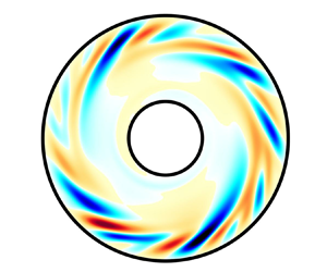
When the perturbations develop further to form convection, a statistically steady state can be found. In this section, we focus on the flow structures in this state. Figure 9 shows some typical snapshots of the instantaneous temperature field on the  $r-\varphi$ plane with increasing shear strength under $\eta =0.3$ and $0.7$ at $Ra=10^6$. Without shear, two pairs of convection rolls appear at $\eta =0.3$ while seven pairs appear at $\eta =0.7$. The fact that more pairs of convection rolls form at larger $\eta$ has been confirmed by previous LSA. Due to the Coriolis force, the cold and hot plumes turn to the right when crossing the bulk region, breaking the symmetry of one roll pair. The single roll of a pair in the plume deflection direction becomes larger and the other becomes smaller (Wang et al. Reference Wang, Jiang, Liu, Zhu and Sun2022). When the shear is applied, the movement direction of the two walls aligns precisely with the rotation direction of the larger roll, thereby further enhancing the asymmetry. Consequently, as the shear strengthens, the convection rolls gradually diminish until they cease to exist.

Figure 9. Typical snapshots of the instantaneous temperature field on the  $r-\varphi$ plane at $Ri_g=\infty,10,5,2,1$ for (a–e) $\eta =0.3$ and ( f–j) $\eta =0.7$. $Ra=10^6$.
Since there are fewer convection rolls for a small radius ratio, they quickly disappear when shear becomes stronger. For  $\eta =0.3$, only one strong cold plume and several hot plumes remain at $Ri_g=5$, as shown in figure 9(c). Due to the high temperature of the bulk regime, the hot plume is not easily observed compared with the cold plume. In fact, there is a rising hot plume immediately adjacent to the cold plume, and the two form a convection roll. With the shear of the boundary, the plumes will move azimuthally. The number of hot temperature perturbations near the outer wall seems to be greater than that of the temperature perturbations near the inner wall because the surface of the outer cylinder is much larger than the surface of the inner cylinder, which is one of the manifestations of the asymmetry in ACRBC. With the further enhancement of the shear, the cold plume disappears, while significant long tilting hot plumes derive from the outer cylinder. This phenomenon again validates the outward shift of the critical modes discovered in the LSA, which indicates that the thermal convection pattern is also affected by the inhomogeneous distribution of the shear, and the influence is more pronounced at small radius ratios.
Under  $\eta =0.7$, since more convection roll pairs exist without shear; their disappearance occurs at smaller $Ri_g$. Until $Ri_g=1$, although no significant convection rolls are present, there are still many plumes detached from both the inner and outer cylinders, as shown in figure 9(j). This is partly due to the large inner wall area of the system with large $\eta$, which therefore allows for more plumes to be generated, and partly because the shear effect is more uniform, which means that the shear on the inner cylinder side is not as strong as that in the case with small $\eta$. When the shear is further enhanced, the plumes on the inner and outer cylinder surfaces are further suppressed as well.
In the snapshots of the temperature field, differences in the bulk temperatures for different  $\eta$ are another concern. For ACRBC without shear, the bulk temperature increases from $\theta _m=0.5$ as $\eta$ decreases from $1$. The enhancement of bulk temperature is caused by the asymmetry of ACRBC in the radial direction, and the effect of the radius ratio on the asymmetric temperature distribution is well described by Wang et al. (Reference Wang, Jiang, Liu, Zhu and Sun2022). In the sheared ACRBC system, this asymmetry has more profound implications for the flow dynamics. In figure 10 we plot the averaged temperature profiles of different $Ri_g$ under $\eta =0.3$ and $0.7$. It can be seen that at weak shear, the bulk temperature at $\eta =0.3$ is larger than that at $\eta =0.7$. With the increase of shear strength, the uniform bulk temperature gradually increases, meanwhile, the uniform bulk area shifts towards $\hat {r}=1$. For small $\eta =0.3$, a significant increase of bulk temperature and the corresponding shift happen at a larger $Ri_g=2$, where the cold plumes totally disappear, as shown in figure 9(d), while, for $\eta =0.7$, the bulk temperature remains nearly constant until $Ri_g=1$, indicating the robust bulk convective mixing. Afterward, the flow suddenly evolves to the laminar and non-vortical state. Again, this is consistent with the LSA results, illustrating that the inhomogeneity of the shear distribution affects the sheared ACRBC at different radius ratios with different intensities in various aspects including stability and flow structures.

Figure 10. Radial distribution of azimuthally and time-averaged temperature  $\langle \theta \rangle _{t,\varphi }$ at different shear strengths for (a) $\eta =0.3$ and (b) $\eta =0.7$. $Ra=10^6$.
4.3. Global transportation
The different flow structures for different  $\eta$ further affect the global transportation in sheared ACRBC. The heat transfer efficiency and the momentum transfer efficiency in the statistically steady state are measured by two Nusselt numbers: $Nu_h$ and $Nu_\omega$, defined as the ratios of the corresponding fluxes of the current system to the fluxes in the laminar and non-vortical flow cases (Eckhardt et al. Reference Eckhardt, Grossmann and Lohse2007; Wang et al. Reference Wang, Jiang, Liu, Zhu and Sun2022; Zhong et al. Reference Zhong, Wang and Sun2023)
 \begin{equation} \left.\begin{gathered} Nu_h=\frac{\sqrt{RaPr}\langle u_r\theta\rangle_{t,\varphi,z}-{\partial\langle\theta\rangle_{t,\varphi,z}/\partial{r}}}{(r\ln(\eta))^{{-}1}},\\ Nu_\omega=\frac{r^3[Ra/Pr\langle u_r\omega\rangle_{t,\varphi,z}-\sqrt{Ra/Pr}{\partial\langle\omega\rangle_{t,\varphi,z}/\partial{r}]}}{2B}, \end{gathered}\right\} \end{equation}
where  $\omega =u_\varphi /r$ is the angular velocity of the fluid, and $B$ is the parameter of the base flow defined in (3.2a,b). Here, $\langle {\cdot } \rangle _{t,\varphi,z}$ represents the temporal-, azimuthal- and axial-averaged value. In ACRBC without shear, i.e. $\varOmega =0$ or $Ri_g=\infty$, $Nu_h$ decreases with decreasing $\eta$ for a fixed $Ra$ (Wang et al. Reference Wang, Jiang, Liu, Zhu and Sun2022). Meanwhile, it is known that shear will suppress the heat transfer efficiency as well (Blass et al. Reference Blass, Zhu, Verzicco, Lohse and Stevens2020; Zhong et al. Reference Zhong, Wang and Sun2023). When shear is introduced in ACRBC, what would be the difference in the relationship of $Nu$ with shear strength at different $\eta$? To make a reasonable comparison of shear strengths for systems with different $\eta$, we still adopt the global Richardson number $Ri_g$ to represent the shear strength here.
The variations of the two Nusselt numbers with  $Ri_g$ at different $\eta$ are illustrated in figures 11(a) and 11(b) for $Ra=10^6$ and in figures 11(d) and 11(e) for $Ra=10^7$. With the increase of shear strength (decreasing $Ri_g$), $Nu_h$ decreases slowly at first and then rapidly when the flow approaches the marginal state. The value $Nu_h-1$ in the figures reflects the extent of heat transfer enhancement compared with heat conduction. This trend holds for different radius ratios and the two Rayleigh numbers. The transition in the rate of decline of $Nu_h$ can be clearly seen in the logarithmic coordinate system of figures 11(a) and 11(d), and exactly corresponds to the vanishing of convection rolls, as shown in figure 9. For example, the rapid decrease of $Nu_h$ occurs when $Ri_g<5$ for $\eta =0.3$ and $Ri_g<1$ for $\eta =0.7$. Therefore, the shear has smaller effects on the heat transfer before the breaking of the large convection rolls. This means that, for large $\eta$ with robust convection, a nearly constant $Nu_h$ can hold for a large range of $Ri_g$, as can be seen in figures 11(a) and 11(d).

Figure 11. Variation of (a,d)  $Nu_h$, (b,e) $Nu_\omega$ and (c, f) $\gamma$ with $Ri_g$ at $\eta =0.3$, $0.5$, $0.7$ and $0.9$. The data in the first row (a–c) are calculated at $Ra=10^6$, while the data in the second row (d–f) are calculated at $Ra=10^7$.
In the buoyancy-dominated regime of sheared ACRBC,  $Nu_\omega$ is smaller than $1$, which means that the drag on the boundaries is smaller than the drag of base flow (Zhong et al. Reference Zhong, Wang and Sun2023). For a weak shear, $Nu_\omega$ even becomes negative, indicating that the large convection rolls push the two cylinders to rotate. Therefore, in figures 11(b) and 11(e), $1-Nu_\omega$ is considered, which represents the role of thermal convection in wall motion. When shear is weak, the values of $Nu_\omega$ are close for different $\eta$. With enhanced shear, $1-Nu_\omega$ yields the same trend as $Nu_h-1$, namely decreasing slowly at first and rapidly afterward. The transition similarly occurs when the convection rolls disappear. Therefore, the global convection mode holds great significance for both heat and momentum transfer in sheared ACRBC.
To further investigate the relationship between heat and momentum transfer, we again adopt the perspective of energy. In the dimensional form, as  $u^*_\varphi /r^*\ll \varOmega ^*_c$ in the buoyancy-dominated regime, the global energy balance of our system can be derived from (2.1) (Eckhardt et al. Reference Eckhardt, Grossmann and Lohse2007; Wang et al. Reference Wang, Jiang, Liu, Zhu and Sun2022; Zhong et al. Reference Zhong, Wang and Sun2023)
 \begin{equation} \varepsilon-\varepsilon_{lam}=\sigma_r^{{-}2}Ta(Nu_\omega-1)+f(\eta)Pr^{{-}2}Ra(Nu_h-1), \end{equation}
where  $\varepsilon =(Ra/Pr)\langle (\partial _iu_j+\partial _ju_i)^2\rangle _{V,t}$ is the dimensionless mean energy dissipation rate, $\varepsilon _{lam}$ is the dimensionless mean energy dissipation rate of the laminar and non-vortical flow, $\sigma _r=(1+\eta )^4/16\eta ^2$ is the quasi-Prandtl number and $f(\eta )={2(\eta -1)}/{(1+\eta )\ln (\eta )}$ is a correction factor for the annular geometry. The two terms on the right side represent the energy injected by shear and buoyancy, respectively. As the momentum Nusselt number $Nu_\omega <1$, the first term on the right side is negative, indicating that the shear consumes energy and only the buoyancy provides. The ratio $\gamma$ of the energy consumed by shear and the energy injected by buoyancy reads
 \begin{equation} \gamma=\frac{\sigma_r^{{-}2}Ta(1-Nu_\omega)}{f(\eta)Pr^{{-}2}Ra(Nu_h-1)}=\frac{-8\eta^2\ln \eta(1-Nu_\omega)}{(1+\eta)(1-\eta)^3(Nu_h-1)}Pr\varOmega^{2}. \end{equation}
Figures 11(c) and 11( f) show how  $\gamma$ varies with $Ri_g$ at different radius ratios for $Ra=10^6$ and $10^7$, respectively. Basically, $\gamma$ increases with decreasing $Ri_g$ in an approximate power law relation. Interestingly, for $Ra=10^6$ and small $Ri_g$, the curves representing different radius ratios, which are separated in the other two figures, collapse together in the $\gamma -Ri_g$ relation, indicating that the energy allocation rules in the flow close to the stable state are similar for different $\eta$. Meanwhile, this implies that $Ri_g$ is not only applied for the initial linear instability but also for the fully developed flow field. At larger $Ri_g$, the shear is weak and the convection rolls are strong; $\gamma$ is larger for smaller $\eta$. The reason for this may be that the nonlinearities of large convection rolls introduce new factors related to $\eta$ to come into play, such as the curvature, Coriolis force and the zonal flow (Wang et al. Reference Wang, Jiang, Liu, Zhu and Sun2022). Consequently, a single $Ri_g$ cannot completely describe the effect of different radius ratios on the heat and momentum transfer of the system. For the cases with $Ra=10^7$, in which the convection rolls are more intense, the curves representing different $\eta$ are always slightly separated. As discussed in § 3, for high $Ra$, the outward shift of the critical mode and the confinement of the azimuthal wavelength make the critical $Ri_g$ vary slightly. Nevertheless, considering the comprehensive results above, $Ri_g$ behaves well in characterizing the overall trend of heat and momentum transfer of sheared ACRBC at different radius ratios.
5. Conclusion
In the present study, we investigate the effect of the radius ratio on the sheared ACRBC system by LSA and DNSs. Guided by the description of Zhong et al. (Reference Zhong, Wang and Sun2023), since the temperature only works as a passive scalar in the shear-dominated regime, we concentrate on the buoyancy-dominated regime of sheared ACRBC, where the quasi-2-D thermal convection is gradually suppressed by increasing imposed shear. Through the LSA, we observe that, as the radius ratio  $\eta$ increases from $0.2$ to $0.95$, the marginal-state curve $Ra_c(\varOmega )$ shifts along the $-\varOmega$ direction, which means a smaller $\varOmega$ is required to stabilize the flow. Considering the inhomogeneity of the shear strength distribution due to the geometric asymmetry, a global Richardson number $Ri_g$ is defined in terms of the most representative local Richardson number. With the newly defined $Ri_g$, the marginal-state curves under different radius ratios collapse together in the parameter domain $(Ra, Ri_g)$, also consistent with the marginal-state curve $Ra_c(Ri)$ of the wall-sheared RBC in the streamwise direction. This demonstrates that the stabilization mechanism in the direction of shear flow is identical for the two systems. In addition, due to the geometrical limitation of the maximum azimuthal wavelength, the marginal-state curves in sheared ACRBC are offset from those of the wall-sheared RBC under high-intensity shear.
The equivalent aspect ratio of the system at low radius ratios is smaller, which allows the system to accommodate fewer roll pairs according to the circular roll hypothesis (Wang et al. Reference Wang, Jiang, Liu, Zhu and Sun2022). When shear is applied, this causes the convection rolls as well as the thermal plumes in the system to disappear more quickly, thus allowing the heat transfer to be drastically suppressed in advance. Meanwhile, the strong asymmetry of the small radius ratio system causes significant disparity in the quantities of hot and cold plumes along with temperature elevation in the bulk region, and the imposition of shear further exacerbates these effects. Interestingly, even if the flow structures differ, the percentage of buoyant energy consumed by shear varies consistently with  $Ri_g$ for systems with different radius ratios. This, in turn, indicates that $Ri_g$ serves as a robust global parameter.
Moreover, apart from geometric asymmetry, strong shear inhomogeneity can have a significant impact on the sheared ACRBC of small radius ratios. In instability analysis, the inhomogeneity of shear leads to the outward displacement of perturbations in critical modes at high Rayleigh numbers. Meanwhile, it also causes the well-mixed convection region to shift outward under strong shear, which is reflected by the asymmetric temperature profiles in the numerical simulations.
By exploring the effect of the radius ratio on the sheared ACRBC system, we successfully match the stabilization mechanism of sheared ACRBC to that of wall-sheared RBC and answer the question as to why a stable regime appears in the former. Shear inhibits the streamwise perturbations and stabilizes the thermal convection, while the asymmetry of the system and the inhomogeneity of the shear distribution can also have an important effect on flow characteristics and stability. Moreover, we note that the global Richardson number we defined for sheared ACRBC works well at a low Rayleigh number, but it is not a good quantitative description of the instability at high Rayleigh numbers. How to quantitatively characterize the outward shift of perturbations and wavelength limitation of the geometry still needs to be explored in the future. In addition, as the thermal flow in this study is still in the classical regime, extending the current investigations to the ultimate regime poses an ongoing challenge. Which radius ratio value is preferable for the ultimate regime study? Does the interaction of shear and buoyancy change under very strong convection? Despite being limited by the huge demand for computational resources, this is an interesting question that deserves future exploration.
Funding
This work was supported by the National Natural Science Foundation of China under grant no. 11988102, and the New Cornerstone Science Foundation through the New Cornerstone Investigator Program and the XPLORER PRIZE.
Declaration of interests
The authors report no conflict of interest.
Appendix A. Linear stability analysis details
Below, we provide more details of the LSA. Following (3.1) and (3.2a,b), the flow field is decomposed into the base flow and perturbation field. Taking the decomposition into the governing equation (2.1), ignoring the nonlinear term and using the normal modes form in (3.3), one can get the resulting equation for the radial shape function  $\boldsymbol {\hat {\psi }}(r)=(\boldsymbol {\hat {u}}(r),\hat {p}(r),\hat {\theta }(r))$
 \begin{align} \left.\begin{gathered} (D+r^{{-}1})\widehat{u_r}+{\rm i}nr^{{-}1}\widehat{u_\varphi}+{\rm i}k\widehat{u_z}=0,\\ \left(s+\frac{{\rm i}nu_0}{r}\right)\widehat{u_r}-\frac{2u_0}{r} \widehat{u_\varphi}={-}D\hat{p}+Ro^{{-}1}\widehat{u_\varphi}+\sqrt{\frac{Pr}{Ra}}\left( \nabla^2\widehat{u_r}-\frac{\widehat{u_r}}{r^2}-\frac{2in\widehat{u_\varphi}}{r^2}\right)\\ \quad -\frac{2(1-\eta)}{(1+\eta)}r \left[\left(1+\frac{2u_0}{Ro^{{-}1}r}\right)^2 \hat{\theta}+\frac{4\theta_0}{Ro^{{-}1}r}\left(1+\frac{2u_0}{Ro^{{-}1}r}\right)\widehat{u_\varphi}\right],\\ \left(s+\frac{{\rm i}nu_0}{r}\right)\widehat{u_\varphi}+\left(Du_0+\frac{u_0}{r}\right) \widehat{u_r}={-}\frac{{\rm i}n}{r}\hat{p}-Ro^{{-}1}\widehat{u_r}+\sqrt{\frac{Pr}{Ra}}\left(\nabla^2\widehat{u_\varphi}- \frac{\widehat{u_\varphi}}{r^2}+\frac{2{\rm i}n\widehat{u_r}}{r^2}\right),\\ \left(s+\frac{{\rm i}nu_0}{r}\right)\widehat{u_z}={-}{\rm i}k\hat{p}+\sqrt{\frac{Pr}{Ra}}\nabla^2\widehat{u_z},\\ \left(s+\frac{{\rm i}nu_0}{r}\right)\hat{\theta}+(D\theta_0)\widehat{u_r}=\frac{1}{\sqrt{RaPr}}\nabla^2\hat{\theta}, \end{gathered}\right\} \end{align}
where operators  $D=\textrm {d}/\textrm {d}r$ and $\nabla ^2=D^2+D/r-n^2/r^2-k^2$ are introduced for simplification. The equations can be transferred into a generalized eigenvalue problem with the eigenvalue $s$ (Kang et al. Reference Kang, Meyer, Mutabazi and Yoshikawa2017), as
 \begin{equation} \mathcal{L}\boldsymbol{\hat{\psi}}(r)=s\mathcal{B}\boldsymbol{\hat{\psi}}(r), \end{equation}
where  $\mathcal {L}$ and $\mathcal {B}$ are the operator matrixes from (A1). The boundary conditions of the generalized eigenvalue problem come from (2.2), which reads
 \begin{equation} \boldsymbol{\hat{u}}(r_i)=\boldsymbol{\hat{u}}(r_o)=0,\quad\hat{\theta}(r_i)=\hat{\theta}(r_o)=0. \end{equation}
Then, this generalized eigenvalue problem is solved by the Chebyshev spectral collocation method. After discretization on Chebyshev–Gauss–Lobatto collocation points, the eigenvalue problem is transferred into calculating the generalized eigenvalues and eigenfunctions of matrixes, which can be easily solved with a small computational cost (Yoshikawa et al. Reference Yoshikawa, Nagata and Mutabazi2013; Meyer et al. Reference Meyer, Yoshikawa and Mutabazi2015). In our work, the number of Chebyshev–Gauss–Lobatto collocation points  $N$ is set at $512$ to guarantee good convergence. After solving the generalized eigenvalue problem, the temporal growth rate $s$ is solved as the eigenvalue, and the corresponding perturbation mode $\boldsymbol {\hat {\psi }}(r)$ is solved as the eigenfunction. The mode with maximum real growth rate $\sigma =real(s)$ over all wavenumber sets $(n,k)$ is the most unstable mode; once $\sigma >0$, the flow is unstable and this perturbation mode grows.
Appendix B. Numerical details
The parameters of the main simulations considered in this work are listed in table 1. The columns from left to right indicate the Rayleigh number  $Ra$, the radius ratio $\eta$, the non-dimensional rotation velocity difference $\varOmega$, the global Richardson number $Ri_g$, the resolution in the radial and azimuthal direction $(N_r, N_\varphi )$, the Nusselt number of heat transfer $Nu_h$ and its relative difference of two halves $\epsilon _{Nu_h}$, the Nusselt number of momentum transfer $Nu_\omega$ and its relative difference of two halves $\epsilon _{Nu_\omega }$ and the posterior check on the maximum grid spacing $\varDelta _g$ by the Kolmogorov scale $\eta _K$ and the Batchelor scale $\eta _B$. The Kolmogorov scale is estimated by the criterion $\eta _K=(\nu /\varepsilon )^{1/4}$, where $\varepsilon$ is the mean energy dissipation rate calculated by (4.2). The statistical errors are estimated by the differences between the first half and the second half, as $\epsilon _{Nu_{h,\omega }}=|(\langle Nu_{h,\omega }\rangle _{0-T/2}-\langle Nu_{h,\omega }\rangle _{T/2-T})/({Nu_{h,\omega }}-1)|$.
Table 1. Simulation parameters.


