


1. Introduction
Mountain glaciers are key indicators and unique demonstration objects of global climate change (Reference HoughtonHoughton and others, 2001). As a consequence, they are an ‘essential climate variable’ in the terrestrial part of the Global Climate Observing System (GCOS/GTOS). The corresponding monitoring network, the Global Terrestrial Network for Glaciers (GTN-G), is run by the World Glacier Monitoring Service (WGMS) in close cooperation with the Global Land Ice Measurements from Space (GLIMS) initiative (Reference BishopBishop and others, 2004; Reference Bamber and KnightBamber, 2006; Reference Kääb and KnightKääb, 2006; cf. GCOS, 2003, 2004; Reference HaeberliHaeberli, 2004). The monitoring network uses an integrated, multi-level strategy, which helps to bridge the gap between detailed local process-oriented studies and global coverage by combining in situ measurements (mass balance, length change) with remote-sensing data and digital terrain information (areas, elevations, topographic parameters, inventories) and numerical modelling (thickness estimates, energy balance, flow modelling). The primary aim of this paper is to illustrate this concept by integrating a rich basis of existing data for the case of the European Alps, where especially dense information has been available through historical times. It thereby first (a) analyzes mass change through time at a sample of individual glaciers as a direct expression of changing energy and mass (precipitation) fluxes between the atmosphere and the Earth surface, and then (b) combines the corresponding results with overall changes in glacier area and volume for the entire mountain chain with a view to corresponding impacts on landscapes, the water cycle, geomorphic processes or natural hazards. The study refers to primary goals of long-term climate-related monitoring programmes, i.e. early detection, model validation and assessing impacts of change. After a brief overview of the multi-level system as defined for GTN-G, examples relating to (a) and (b) as given above are presented, and finally current major challenges for an integrated global glacier monitoring strategy are discussed.
2. The Multi-Level System for GTN-G
The multi-level system as defined for GTN-G follows the global hierarchical observing strategy (GHOST) and was first described by Reference Haeberli, Cihlar and BarryHaeberli and others (2000). It attempts to connect intensive local studies on individual glaciers with coverage of large glacier ensembles at the global scale by integrating the following steps (see Reference HaeberliHaeberli, 2004, for a more detailed discussion):
extensive and process-oriented glacier mass-balance and flow studies within the major climatic zones for calibrating numerical models (there are about ten glaciers with intensive research and observation activities that represent such sites; Storglaciären, northern Sweden, is an example (Reference Haeberli, Noetzli, Zemp, Baumann, Frauenfelder and HoelzleHaeberli and others, 2005));
regional glacier mass changes within major mountain systems, observed with a limited number of strategically selected stakes/pits combined with precision mapping at about decadal intervals: on about 50 glaciers annual mass-balance studies reflect regional patterns of glacier mass changes (Reference Haeberli, Noetzli, Zemp, Baumann, Frauenfelder and HoelzleHaeberli and others, 2005); however, spatial coverage still shows gaps in some of the major mountain systems such as the Himalaya, the New Zealand Alps and Patagonia (Reference Dyurgerov and MeierDyurgerov and Meier, 1997);
long-term observations of glacier length changes: a minimum of about ten sites within each major mountain range should be selected to represent different glacier sizes and dynamic responses; the representativeness of glaciers can be assessed by intercomparison (within and between regions) of geometrically comparable glaciers, dynamic fitting of glacier flow models to long time series of measured cumulative length change (Reference OerlemansOerlemans and others, 1998), and mass-change reconstructions using concepts of mass conservation (Reference Hoelzle, Haeberli, Dischl and PeschkeHoelzle and others, 2003);
glacier inventories repeated at intervals of a few decades using satellite remote sensing (continuous upgrading and analyses of existing and newly available data; modelling of data following the scheme developed by Reference Haeberli and HoelzleHaeberli and Hoelzle (1995)).
Basic elements of these recommendations have been explained before (Reference Haeberli, Hoelzle and SuterHaeberli and others, 1998) but still need further evaluation and testing. Strategically selected stakes/pits (a minimum of three) for determining high-frequency (annual) mass change in connection with repeated mapping should, for instance, document (a) effects near the equilibrium line where the largest glacier areas tend to be and where mass-balance sensitivity is largely determined (Reference Braithwaite and KnightBraithwaite, 2006); (b) the balance at the glacier terminus, which is used to convert cumulative long-term length change into average long-term mass change (Reference Hoelzle, Haeberli, Dischl and PeschkeHoelzle and others, 2003); and herewith (c) the mass-balance gradient in the ablation area as the main expression of climate sensitivity and flow forcing (Reference Dyurgerov and DwyerDyurgerov and Dwyer, 2001). Long-term observations at isolated index stakes without repeated mapping of the entire glacier are not recommended, because they cannot easily be related to other components of the integrated monitoring strategy and may even be confusing for a wider public. Concerning length change, geometry largely determines dynamic response characteristics (Fig. 1) and is clearly more important than local neighbourhood: small, low-stress cirque glaciers (‘glaciers réservoirs’) react to high-frequency signals but with small overall length change; mountain glaciers with intermediate size on relatively steep slopes (‘glaciers évacua-teurs’) filter out short-term climate influences but clearly show changes at decadal time intervals (e.g. in the Alps, the intermittent readvances and mass gains around 1920 and 1965–80); while long valley glaciers provide the strongest climate signals, but with a time resolution at the century scale. In general, glaciers with surge behaviour, calving instabilities or ablation by ice avalanching, but also glaciers subject to volcanic influences, heavily covered by debris or resting on thick sediment beds (causing corresponding longterm changes in bed level), are not suitable for climatic inferences. As an example for the European Alps, the long series of isolated local seasonal balance (accumulation) observations at two sites on Claridenfirn (starting in 1917) must be disregarded in this respect, as Claridenfirn is mostly an accumulation area with ice avalanches constituting the main ablation process, prohibiting geometric changes and, hence, making realistic mass-balance determinations impossible for simple topographic reasons.

Fig. 1. Cumulative length changes since 1900 of three characteristic glacier types in the Swiss Alps. Small cirque glaciers such as Pizolgletscher have low basal shear stresses and directly respond to annual mass-balance and snowline variability through deposition/melting of snow/firn at the glacier margin. Medium-sized mountain glaciers such as Glacier de Trient flow under high basal shear stresses and dynamically react to decadal mass-balance variations in a delayed and strongly smoothed manner. Large valley glaciers such as Aletschgletscher may be too long to dynamically react to decadal mass-balance variations, but exhibit strong signals of secular developments. Considering the whole spectrum of glacier response characteristics gives the best information on secular, decadal and annual developments. Data from WGMS.
Numerical modelling at various levels of complexity and remote-sensing information should help to extend the measured data in space and time, i.e. bridging the gap between local studies and global application. In this respect, there is a large potential for the use of modern geoinformatic techniques (i.e. geographic information systems (GIS)) that allow extraction of data and calculation of statistics for thousands of glacier entities automatically (Reference Kääb, Paul, Maisch, Hoelzle and HaeberliKääb and others, 2002; Reference Paul, Kääb, Maisch, Kellenberger and HaeberliPaul and others, 2002; Reference PaulPaul, 2004). The suite of numerical models that can be applied reaches from (a) simple but robust parameterization schemes (Reference Haeberli and HoelzleHaeberli and Hoelzle, 1995; Reference Hoelzle, Chinn, Stumm, Paul, Zemp and HaeberliHoelzle and others, 2007) to (b) more complex, physically based assessments (Reference Hoelzle, Haeberli, Dischl and PeschkeHoelzle and others, 2003) to (c) distributed glacier energy-balance models of varying complexity (e.g. Reference OerlemansOerlemans, 1992; Reference Arnold, Willis, Sharp, Richards and LawsonArnold and others, 1996; Reference Klok and OerlemansKlok and Oerlemans, 2002; Reference Machguth, Eisen, Paul and HoelzleMachguth and others, 2006b) and to (d) coupled mass-balance–glacier-flow models (e.g. Reference GreuellGreuell, 1992; Reference OerlemansOerlemans, 1997; Reference HubbardHubbard and others, 2000). In particular, (c) has the potential to calculate climate-change effects on mountain glaciers from (downscaled) meteorological data as computed by regional climate models (RCMs) and other gridded input datasets (Reference Paul, Kotlarski and HoelzlePaul and others, 2006; cf. Reference Salzmann, Frei, Vidale and HoelzleSalzmann and others, 2007, for analogous permafrost modelling). The following illustrates various methods of assessing past, current and future glacier mass changes by combining field data and/or remote-sensing information with numerical modelling. Such approaches build on a robust understanding of some of the most fundamental aspects related to the process chain linking climate and (medium-sized mountain) glaciers:
air temperature predominates in the temporal variability of the energy balance (e.g. Reference Braithwaite and KnightBraithwaite 2006; Reference Braithwaite and RaperBraithwaite and Raper, 2007; and references therein) and causes mass balances to be spatially correlated over large regions (spanning several hundred kilometres: Reference Letréguilly and ReynaudLetréguilly and Reynaud, 1990; Reference Cogley and AdamsCogley and Adams, 1998), an effect which is most likely due to combined influences from sensible-heat and longwave radiation (Reference OhmuraOhmura, 2001);
patterns of long-term precipitation have a strong influence on glacier variability in space (mass turnover, englacial temperatures, relation to periglacial permafrost, mass-balance sensitivity: e.g. Reference Letréguilly and ReynaudOerlemans, 2001; Reference Haeberli, Burn and SidleHaeberli and Burn, 2002; Reference Braithwaite and KnightBraithwaite, 2006) but change rather weakly in time (over decadal to centennial periods) and hence appear to have only secondary effects with respect to recent glacier fluctuations (e.g. Reference OerlemansOerlemans, 2005; Schöner and Böhm, 2007);
dynamic response times for complete adjustment to equilibrium conditions are slope-dependent, for the simple reason that they depend on ice thickness divided by the balance at the terminus (Reference Jóhannesson, Raymond and WaddingtonJóhannesson and others, 1989) and the balance at the terminus (in steady-state condition) tends towards zero with slope decreasing towards zero (Reference Haeberli and HoelzleHaeberli and Hoelzle, 1995); characteristic values are on the order of decades for typical (relatively thin and steep) mountain glaciers but may reach centuries for large (thick), flat glaciers;
geometric changes over such time intervals are primarily governed by mass conservation (Reference GreuellGreuell, 1992; Reference Boudreaux and RaymondBoudreaux and Raymond, 1997; Reference Hoelzle, Haeberli, Dischl and PeschkeHoelzle and others, 2003) rather than by specific aspects of glacier flow;
albedo and mass-balance/altitude feedbacks can have strong impacts (Reference Paul, Machguth and KääbPaul and others, 2005; Reference Raymond and NeumannRaymond and Neumann, 2005) and may even cause self-reinforcing ‘runaway effects’ (downwasting rather than retreat of glaciers where ‘vertical’ thickness loss is faster than the capacity of a glacier to ‘horizontally’ retreat); increasing debris cover, on the other hand, tends to decouple glaciers from atmospheric influences and can markedly slow down ice melting and strongly retard tongue retreat (Reference Smiraglia, Diolaiuti, Casati and KirkbrideSmiraglia and others, 2000). Sometimes, debris-covered glacier tongues may even lose contact with the main glacier and develop into a body of ‘dead ice’. Length-change measurements make little sense in such cases.
3. Mass Change Through Time at Individual Glaciers
3.1. Mass-balance measurements
Mass-balance measurements in GTN-G combine the direct glaciological method (stakes and pits: point measurements with high time resolution) with the photogrammetric/geodetic method (repeated mapping: survey of the entire glacier at lower time resolution) for optimal information and calibration. Field measurements are either carried out with extended stake/pit networks for detailed process understanding and development of numerical models, or use cost-saving approaches with reduced numbers of strategically chosen ‘index’ stakes, providing gross regional indications of change (Reference Haeberli, Hoelzle and SuterHaeberli and others, 1998).
Photogrammetrically/geodetically determined volume changes and glacier mass balances are available in the European Alps back to the late 19th century (Table 1). Uninterrupted in situ measurements since 1967 of mass balance at nine Alpine glaciers are shown in Figure 2. Near-equilibrium conditions until 1981 were followed by very strong and continued if not accelerating mass loss (0.7mw.e. a–1; trend of increase in mass loss 0.03– 0.04 mw.e. a–2). During the first 5 years of the 21st century, mean annual mass losses have been close to 1 mw.e. a–1. The hot, dry summer of 2003 alone caused a record mean loss of 2.45 mw.e., roughly 50% above the previous record loss in 1998.

Fig. 2. Annual (a) and cumulative (b) mass balance of nine glaciers with uninterrupted mass-balance determination (for the entire glacier) in the European Alps (Saint-Sorlin and Sarennes, France; Gries and Silvretta, Switzerland; Careser, Italy; Hintereis, Kesselwand, Vernagt and Sonnblick, Austria). Data from WGMS. The light dashed lines show an average mass loss of nearly 18 m, or 716 mma–1, (b) and an average increase in mass loss of 34 mma–2 (a) since 1980. The Silvretta values may be systematically too positive and should be corrected in the near future.
Table 1. Geodetically/photogrammetrically determined secular mass balances of alpine glaciers

It must be kept in mind that climatic conditions which remain constant in time would lead to geometric adjustment of glaciers to new equilibrium states and a corresponding zero balance. Continued non-zero balances indicate ongoing climate forcing (assuming feedbacks from albedo, elevation change, debris cover or dry/wet calving do not affect mass balance for the considered glaciers), and increasing deviations from zero balances reflect accelerating change. True values for continued or accelerated forcing would have to be modelled for glacier areas remaining constant in time (cf. Reference Elsberg, Harrison, Echelmeyer and KrimmelElsberg and others, 2001; Reference Harrison, Elsberg, Cox and MarchHarrison and others, 2005), an important future possibility for distributed energy- and mass-balance models.
3.2. Mass-balance reconstructions
Mass-balance values during earlier periods must be reconstructed. Models of variable complexity are available for this purpose. Information on cumulative glacier length changes thereby plays a key role for calibration and validation. For the time since the end of the Little Ice Age around 1850, reconstructions have been based on (a) a straightforward continuity consideration applied to cumulative length changes (Reference Haeberli and HoelzleHaeberli and Hoelzle, 1995; Reference Hoelzle, Haeberli, Dischl and PeschkeHoelzle and others, 2003), and (b) neural networks using present-day mass-balance measurements together with meteorological data that reach farther back in time (Reference Steiner, Walter and ZumbühlSteiner and others, 2005). The two approaches are completely independent and both provide long-term mass-balance averages of –0.25 to –0.3mw.e. a–1, i.e. three to four times less than the most recently observed values. The generally observed retreat of Alpine glacier tongues leaves no doubt that these secular trends and values are representative for the entire mountain chain. Backward reconstructions beyond the mid-19th century are much less homogeneous, especially with respect to temporal changes. This effect so far remains unexplained, but may relate to the fact that statistical models are calibrated with direct measurements on glaciers of already reduced size but then extrapolated for periods with considerably larger glaciers and, most likely, different sensitivities and response characteristics.
The continuity approach (a) was also applied to longer-term cumulative length changes of Grosser Aletschgletscher, Switzerland, (Reference Haeberli and HolzhauserHaeberli and Holzhauser, 2003) which was reconstructed in detail from historical documents, moraine dating and fossil trees for the past 3500 years (Reference Holzhauser, Magny and ZumbuhlHolzhauser and others, 2005). Over the past two millennia, characteristic century to half-century mass-balance averages (mean ±0.3 and maximum ±0.5mw.e. a–1) are comparable to the loss rates since the Little Ice Age and they were far below those observed since 1981. In fact, the mass losses observed since the mid-1980s (about 0.75 mw.e. a–1) exceed the maximum, and even double the maximum, characteristic long-term loss rates during the past two millennia (Fig. 3). Such comparisons help to confirm the spatial representativeness of half-centennial to centennial mass-balance averages with their uncertainty range or variability in sensitivity (roughly ±50% of the calculated mean) as a function of individual glacier geometry (hypsography) and local to regional differentiation of climate forcing (Reference Haeberli and HoelzleHaeberli and Hoelzle, 1995; Reference Haeberli and HolzhauserHoelzle and others, 2003).

Fig. 3. Measured and reconstructed mass balances in the European Alps for (a) the past 2000 years and (b) the past 500 years. Data from WGMS (measured thickness change 1890–2000 and mass balance 1967–2004), Reference Steiner, Walter and ZumbühlSteiner and others (2005) (neural networks; last 500 years) and Reference Haeberli and HolzhauserHaeberli and Holzhauser (2003) (continuity model; past two millennia); cf. also Tables 3 and 4 in the Appendix. The essential information on rates of mass change is reflected in the slopes of the curves; the vertical position of the curves is somewhat arbitrary.
Distributed mass-balance models taking into account local effects such as those from topography, local albedo or snow redistribution by wind and avalanches not only narrow the uncertainty by providing safer estimates of ablation at glacier margins in complex topography, but also help to explain the variable climate sensitivity of individual glaciers (e.g. Reference Klok and OerlemansKlok and Oerlemans, 2002; Reference Machguth, Eisen, Paul and HoelzleMachguth and others, 2006b; Reference Paul, Machguth, Hoelzle, Salzmann, Haeberli, Orlove, Wiegandt and LuckmanPaul and others, in press). Realistic estimation of local precipitation and accumulation patterns (cf. Reference Machguth, Paul, Hoelzle and HaeberliMachguth and others, 2006a) thereby remains the primary challenge, influencing the results considerably more than the relatively well-established calculation of the summer energy balance and the resulting ablation patterns (e.g. Reference HockHock, 2005).
3.3. Consequences of the recent mass loss
The increasingly fast mass and ‘vertical’ thickness loss clearly points to an accelerating trend in climatic forcing. The corresponding additional energy flux calculated as the latent heat of the disappearing ice (around 10Wm–2 as an average of the past 5 years) is about twice the estimated present-day radiative forcing alone (severalWm–2; Reference WildWild and others 2005) and most probably relates to important feedback mechanisms. The albedo feedback from disappearing firn in former accumulation areas has long-term consequences: the extreme summer 2003 essentially eliminated all remaining firn from the surface of many smaller and medium-sized glaciers. In addition, these bare surfaces strikingly darkened because of wind-blown dust from the snow-free and dry mountains around. As a consequence, the melting snow cover in springtime now uncovers a low-albedo surface, which suffers from strongly enhanced melt (Reference Paul, Machguth and KääbPaul and others, 2005).
Rapid thickness loss with limited tongue retreat also reduces driving stresses and flow within the ice. In such a situation, effects from mass-balance/altitude feedback become fundamentally important, especially for large, thick glaciers which cannot lose exposed ablation areas fast enough. Thereby, total surface lowering (integrated over time) must be compared with the mass-balance/altitude gradient. Due to glacier dynamics, local surface lowering can be considerably more rapid than local ablation (negative mass balance) alone; it represents a cumulative phenomenon which can lead to irreversible runaway effects (‘downwasting’ or even ‘collapse’ rather than ‘retreat’). Observed and reconstructed mass losses are therefore also a function of glacier size (Reference Hoelzle, Haeberli, Dischl and PeschkeHoelzle and others, 2003), with large glaciers reducing their thickness more rapidly than small ones. Morphological phenomena of downwasting (flat longitudinal and concave transversal surface profiles, abundant debris cover, collapse holes above subglacial drainage channels, lake formation) have now become visible on many glacier tongues (Fig. 4). With continued thickness losses of 1 mw.e. a–1 or even more, the glaciers with longterm mass-balance time series may disappear within a few decades from now (cf. the experiments with distributed modelling of equilibrium-line altitudes by Reference Zemp, Haeberli, Hoelzle and PaulZemp and others (2006, Reference Zemp, Hoelzle and Haeberli2007) or with dynamically fitted mass-balance/flowmodels by Reference OerlemansOerlemans and others, 1998). This constitutes a serious challenge for long-term monitoring programmes (Reference Paul, Kääb and HaeberliPaul and others, 2007b).

Fig. 4. Roseggletscher in the eastern Swiss Alps, with a collapse hole on its thin tongue. Photo by C. Rothenbühler, summer 2003.
4. Changes in Total Alpine Glacier Cover
4.1. Assessment of total glacier volume
With the compilation of glacier inventories, treatment of entire mountain ranges became possible by combining time series measured at selected glaciers with statistical information on the whole glacier ensemble at suitable time slices. The first calculations for the European Alps as a pilot study for worldwide applications have already indicated the dramatic overall loss in glacier cover for the past century and even more so for realistic scenarios of atmospheric temperature rise during the 21st century (Reference Haeberli and HoelzleHaeberli and Hoelzle, 1995). A primary challenge with such efforts is the realistic estimation of glacier thickness and corresponding ice volumes. The often-used volume/area scaling (Reference Bahr, Meier and PeckhamBahr and others, 1997) is problematic, as it correlates a statistical variable (area) with itself (area in volume) and, hence, suppresses the large scatter (roughly 30% standard deviation for mountain glaciers) in area/thickness relations, which are statistically more reasonable.
A more process-oriented approach applies geometry-dependent driving stresses in combination with mass turnover as defined by the mass-balance gradient and the altitudinal extent of glaciers (Reference Haeberli and HoelzleHaeberli and Hoelzle, 1995). An even simpler and astonishingly elegant consideration assumes that relative volume change is closely comparable to relative area change, because mean glacier thickness (averaged for the changing glacier area) tends to remain constant (even with pronounced overall changes in glacier mass!): by calculating total volume loss from mass-balance time series and mean area during the investigated time interval, and by assuming that percentages in area loss correspond to percentages in volume loss, total volume can be directly approximated (Reference Paul, Kääb, Maisch, Kellenberger and HaeberliPaul and others, 2004). Results for the total glacier volume in the Alps from the three approaches differ by about ±20% around a mean (100–140km3 for the 1970s; Reference Zemp, Haeberli, Hoelzle and PaulZemp and others, 2006), but have their specific advantages: the area/thickness relation is the easiest to apply; the driving-stress solution enables the best understanding of individual thickness variability; while the ‘area–volume percentage’ solution may provide the safest overall estimate.
4.2. Calculation of ongoing volume changes
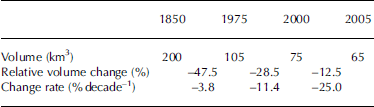
Best estimates for total volumes and volume changes (Table 2; cf. Reference HaeberliHaeberli and others, 2004; Reference Paul, Kääb, Maisch, Kellenberger and HaeberliPaul and others, 2004; Reference Zemp, Haeberli, Hoelzle and PaulZemp and others, 2006) show that glaciers in the European Alps lost about half their total volume (roughly 0.5% a–1) between 1850 and around 1975, another 25% (1% a–1) of the remaining amount between 1975 and 2000, and an additional 10–15% (2–3% a–1) in the first 5 years of this century. The latter estimate is obtained from the mean value of the mass-balance observations at nine Alpine glaciers in combination with the new satellite-derived glacier areas from 1998/99 (Reference PaulPaul, 2004) and a simple model of calculating total glacier volume from mean thickness (Reference Maisch, Wipf, Denneler, Battaglia and BenzMaisch and others, 2000).
Table 2. Estimated ice volumes in 1850, 1975, 2000 and 2005, and changes in the European Alps. The increase in volume-change rates indicates continued or even enhanced climate forcing, but might also be influenced by the different lengths of the periods considered. Data from Reference Zemp, Haeberli, Hoelzle and PaulZemp and others (2006)
Completely new perspectives are coming up with repeated satellite-derived digital terrain models. Even though problems of resolution and accuracy must be carefully evaluated (Reference Berthier, Arnaud, Vincent and RémyBerthier and others, 2006), relative changes as an expression of variable sensitivities can be investigated and used to assess how representative mass-balance time series from selected glaciers are and how they can be best extrapolated to the entire mountain range. Preliminary results from the Swiss Alps indicate a trend towards more negative balances on large, flat glaciers than on smaller ones (Fig. 5).

Fig. 5. Changes in glacier elevation in the region of Zermatt, Swiss Alps, with Gomergletscher at the lower right, from differencing the SRTM3 DEM (resampled to 25 m) from the year 2000 and the swisstopo DEM25 L1 from about 1985. Irregular black areas indicate data voids in the SRTM DEM, which are usually located outside the glacier perimeter. The grey values denote elevation changes from –80m (darkest grey value) to +10m (brightest grey value) and are plotted in classes of half standard deviations. North is at top and image width is 38 km.
4.3. Calculation of potential future changes
Extrapolation for the future based on scenarios of atmospheric warming and relations between mass balance and temperature/precipitation at the equilibrium-line altitude (ELA) as calibrated with long-term mass-balance measurements and gridded climatologies leave no doubt that in such climate scenarios most of the glacier cover in the European Alps is likely to disappear within decades (Reference Zemp, Haeberli, Hoelzle and PaulZemp and others, 2006, Reference Zemp, Hoelzle and Haeberli2007).
Modern data from satellite images as combined with digital terrain information (Reference Kääb, Paul, Maisch, Hoelzle and HaeberliKääb and others, 2002; Reference Paul, Kääb, Maisch, Kellenberger and HaeberliPaul and others, 2002, Reference Paul, Maisch, Rothenbuühler, Hoelzle and Haeberli2007a) greatly enhance the possibilities for numerical modelling and visualization of large samples. Figure 6 is an attempt to combine hypsographic modelling with digital glacier outlines, a satellite image and a digital elevation model (DEM) to visualize a likely sequence of individual glacier decay for a larger region within the Alps. Thereby, simple geometrical rules like a steady-state accumulation-area ratio (AAR) of 0.6 and parameterizations of the ELA sensitivity to temperature change are assumed (Reference Paul, Maisch, Rothenbuühler, Hoelzle and HaeberliPaul and others, 2007a). Such dramatic changes will have strong and predominantly negative impacts on landscape evolution, water supply, erosion/sedimentation, slope stability and natural hazards. Monitoring and spatio-temporal modelling of glacier changes must help with anticipating and mitigating the consequences of such extreme deviations from our historical–empirical knowledge basis and from Holocene conditions of dynamic equilibria.

Fig. 6. Glacier extent for the Aletsch region in 1973 (black outlines) and modelled extent for six shifts of the steady-state ELA using an AAR of 0.6. The legend gives the greyscale that will disappear due to the corresponding shift in ELA. For an ELA rise of 600 m, only the darkest regions will remain. The background is a Landsat satellite image acquired at 31 August 1998. Landsat data © Eurimage/Swiss National Point of Contact for Satellite Images (NPOC).
5. Perspectives and Future Tasks
Several further applications of the multi-level glacier monitoring strategy can be envisaged for the future:
Validation of length change measurements over longer periods from comparisons with satellite data and the related extension of the currently annually measured sample to other remote but climatically interesting regions which are still underrepresented in the existing observational network (e.g. Patagonia and Tierra del Fuego; central Asian high mountains; New Zealand; or the glaciers around Greenland and on Arctic islands (Reference Paul and KääbPaul and Kääb, 2005)). This would also allow a rough first-order estimate of the related long-term mass changes in such regions (cf. Reference Hoelzle, Haeberli, Dischl and PeschkeHoelzle and others, 2003, 2007).
Assessment of firn lines from (maybe annual) satellite data (e.g Reference Rabatel, Dedieu and VincentRabatel and others, 2005) over large areas, and calculation of the related glacier mass balance by comparison with results from distributed mass-balance models.
Application of such distributed mass-balance models over entire mountain ranges (Reference Machguth, Paul, Hoelzle and HaeberliMachguth and others, 2006a; Reference Paul, Machguth, Hoelzle, Salzmann, Haeberli, Orlove, Wiegandt and LuckmanPaul and others, in press) by incorporating extrapolated and gridded datasets of the required input parameters (e.g. precipitation, albedo, potential global radiation) for solving the problems in the accumulation area, which are not obvious if only glacier melt is calculated and models are applied to (e.g. Reference Arnold, Willis, Sharp, Richards and LawsonArnold and others, 1996; Reference Brock, Willis, Sharp and ArnoldBrock and others, 2000) or tuned for individual glaciers (e.g. Reference Klok and OerlemansKlok and Oerlemans, 2002).
Extrapolation of mass-balance measurements at individual ablation stakes and snow pits from such distributed models instead of the simple regressions applied today could presumably help to obtain more realistic mass-balance profiles, as local topographic variability could be much better taken into account (e.g. Reference Arnold, Rees, Hodson and KohlerArnold and others, 2006).
Direct use of output from regional climate models (after appropriate downscaling) to run mass-balance models instead of the sensitivity studies usually applied. This would help to assess the impacts of future climate change (including a changed variability) much more realistically (Reference Paul, Kotlarski and HoelzlePaul and others, 2006).
The approaches and examples presented here demonstrate the large potential of assessing climate-change effects on entire mountain ranges by combining field data with remote-sensing information and numerical modelling. Therefore, two of the most important tasks are the compilation of digital glacier outlines and DEM data at appropriate spatial resolution and on a global scale. While for the latter the near-global availability of the ~90m (30m in the US) resolution Shuttle Radar Topography Mission (SRTM) DEM (e.g. Reference Rabus, Eineder, Roth and BamlerRabus and others, 2003) is a huge step forward (if not a quantum leap), the compilation of digital glacier outlines from remote-sensing data (or digitizing of former inventories) is still in its early stages. The GLIMS project (e.g. Reference BishopBishop and others, 2004; Reference KargelKargel and others, 2005) certainly marks an important starting point, but, due to the small swath width of the Advanced Spaceborne Thermal Emission and Reflection Radiometer (ASTER) sensor (i.e. one-ninth of the Landsat Thematic Mapper (TM)/Enhanced Thematic Mapper Plus (ETM+)), compilation of the data over larger glacierized regions with frequent cloud cover (Himalaya, Canadian Arctic Archipelago, Alaska, etc.) will take additional time. This time should be utilized to communicate about, and finally agree on, standards for glacier definition that support the glacier delineation process, especially with respect to problems in the accumulation area (contributing slopes and hanging glaciers), near flat firn divides or with glaciers splitting up when decaying and retreating, but are still commensurable with existing standards in order to enable comparison with earlier inventories.
6. Conclusions
Integrated use of long-term in situ measurements, satellite images, digital terrain information and numerical models enables overall as well as locally differentiated assessments of ongoing climate-change effects on glacier covers of entire mountain ranges. The mass and volume losses of glaciers in the European Alps are not only fast but seem to be clearly accelerating. This acceleration trend is not only due to accelerated climatic forcing but includes strongly reinforcing feedback mechanisms (albedo, mass balance/altitude) and could lead to near-complete deglaciation of the Alps during the coming decades and the present century. High priority for future research should be given to similar assessments concerning other mountain regions with less dense data and/or shorter time series, and to assessing environmental consequences of such dramatic deviations from past conditions and near-equilibrium states.
Acknowledgements
This study is funded mainly by the Swiss Federal Office of Education and Science (BBW-Contract 901.0498-2) within the European Union programme ALP-IMP (contract EVK2-CT-2002-00148). D. Steiner kindly provided the Aletsch mass-balance data as reconstructed using neural networks. B. Brock, C. Stokes, R. Braithwaite and an anonymous reviewer provided constructive comments which helped improve the paper. We thank the national correspondents and principal investigators of the WGMS for collection and free exchange of important data over many years.
Appendix
Table 3. Thickness changes from selected Alpine glaciers 1889–2000. Compilation and calculation from data of WGMS (http://www.wgms.ch) and Reference Finsterwalder and RentschFinsterwalder and Rentsch (1981)

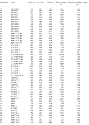

Table 4. Decadal mean annual thickness change of selected Alpine glaciers (calculated from Table 3), 1890–1999. In addition, decadal standard deviations and number of included glaciers are given


