


Introduction
Based on their depth, shallow-water systems are those that occur at depths less than 200 m (Prol-Ledesma et al., Reference Prol-Ledesma, Dando and de Ronde2005; Tarasov et al., Reference Tarasov, Gebruk, Mironov and Moskalev2005). This depth coincides with the maximum depth that the natural light can penetrate in the ocean; although natural light can penetrate deeper under the right conditions, significant light is rarely experienced beyond 200 m (Garrison & Ellis, Reference Garrison and Ellis2016). Shallow-water hydrothermal systems present a gaseous phase, absent in deep-sea hydrothermal systems (Tarasov et al., Reference Tarasov, Gebruk, Mironov and Moskalev2005), as a result, in the past they were called gasohydrothermal vents (Dando et al., Reference Dando, Hughes, Leahy, Niven, Taylor and Smith1995). Most of these hydrothermal systems are associated with volcanic arcs, so the gases are enriched in volcanic volatiles, which causes more acidic fluids and leaching of Mg and other elements, particularly metals, from host rocks (Yang & Scott, Reference Yang and Scott1996; Reeves et al., Reference Reeves, Seewald, Saccocia, Bach, Craddock, Shanks, Sylva, Walsh, Pichler and Rosner2011).
Shallow-water hydrothermal systems are also characterized by very low hydrogen sulphide (H2S) concentrations and smooth horizontal temperature gradients that are not as steep as in deep-sea hydrothermal systems, as had been recorded in some submarine hydrothermal systems around islands such as Vulcano (Italy), Ischia (Italy) and Faial (Azores, Portugal), and also in Milne Bay Province (Papua New Guinea) (Price & Giovannelli, Reference Price and Giovannelli2017). In addition, some shallow-water systems are being used as natural laboratories to study the effects of ocean acidification on biota and microbiota (Hall-Spencer et al., Reference Hall-Spencer, Rodolfo-Metalpa, Martin, Ransome, Fine, Turner, Rowley, Tedesco and Buia2008; Fabricius et al., Reference Fabricius, Langdon, Uthicke, Humphrey, Noonan, De'ath, Okazaki, Muehllehner, Glas and Lough2011; Engel et al., Reference Engel, Hallock, Price and Pichler2015), since CO2 and H2S emissions in shallow hydrothermal systems found in seawater with dissolved oxygen are oxidized to form sulphuric acid $( {{\rm H}_ 2{\rm S}{\rm O}_ 4} )$ and carbonic acid $( {{\rm H}_ 2{\rm C}{\rm O}_ 3} )$
 , which cause a drop in the pH levels of the seawater adjacent to hydrothermal vents and have been shown to remove or dissolve nearby carbon-secreting organisms, leading to potentially dramatic changes in the coastal marine ecosystem in terms of richness and abundance (Hall-Spencer et al., Reference Hall-Spencer, Rodolfo-Metalpa, Martin, Ransome, Fine, Turner, Rowley, Tedesco and Buia2008).
The infauna is better known in shallow-water than in deep-sea systems (Tarasov et al., Reference Tarasov, Gebruk, Mironov and Moskalev2005). It is worth highlighting that nematodes are the common denominator in both systems, and the highest abundances have been reported in shallow systems, such as in a shallow-water hydrothermal system of Milos Island in the Aegean Sea (Thiermann et al., Reference Thiermann, Windoffer and Giere1994; Dando et al., Reference Dando, Hughes, Leahy, Niven, Taylor and Smith1995), and in the Kraternaya Bight on the Kuril Islands in the Russian Federation (Tarasov, Reference Tarasov1999). The lowest abundances are seen in deep-sea systems, such as the deep-sea system of the North Fiji Basin (Vanreusel et al., Reference Vanreusel, Van Den Bossche and Thiermann1997).
Regarding the fauna of shallow-water systems, the presence of species that are also found in anthropogenically contaminated environments is frequent; one of these opportunistic or highly tolerant to stressful environments species groups is the capitellid polychaetes (Tulkki, Reference Tulkki1968; Fauchald & Jumars, Reference Fauchald and Jumars1979; Gamenick et al., Reference Gamenick, Abbiati and Giere1998; Tsutsumi et al., Reference Tsutsumi, Wainright, Montani, Saga, Ichihara and Kogure2001; Tarasov et al., Reference Tarasov, Gebruk, Mironov and Moskalev2005).
The study of shallow-water hydrothermal systems can help in the understanding of various biogeochemical processes, to establish the differences between continental and submarine hydrothermal activity, in the formation of mineral deposits and the geochemical cycle of elements in the oceans (Prol-Ledesma & Canet, Reference Prol-Ledesma and Canet2014). They are usually related to coastal volcanic activity (Tarasov et al., Reference Tarasov, Gebruk, Mironov and Moskalev2005), but they can also be found on continental margins affected by active processes of tectonic extension (Prol-Ledesma & Canet, Reference Prol-Ledesma and Canet2014), as is the case of Mexico, where a site is known in Punta Mita, Nayarit (Núñez-Cornú et al., Reference Núñez-Cornú, Prol-Ledesma, Cupul-Magaña and Suárez-Plascencia2000; Rodríguez-Uribe et al., Reference Rodríguez-Uribe, Núñez-Cornú, Chávez-Dagostino and Trejo-Gómez2020), and four sites on the coast of Baja California Peninsula: Punta Banda (Vidal et al., Reference Vidal, Vidal and Isaacs1978), Bahía Concepción (Prol-Ledesma et al., Reference Prol-Ledesma, Canet, Torres-Vera, Forrest and Armienta2004), Los Cabos (Prol-Ledesma et al., Reference Prol-Ledesma, Carrillo De La Cruz, Torres-Vera and Estradas-Romero2021) and Puertecitos (Arellano-Ramirez et al., Reference Arellano-Ramirez, Kretzschmar and Hernandez-Martinez2017) (Figure 1).
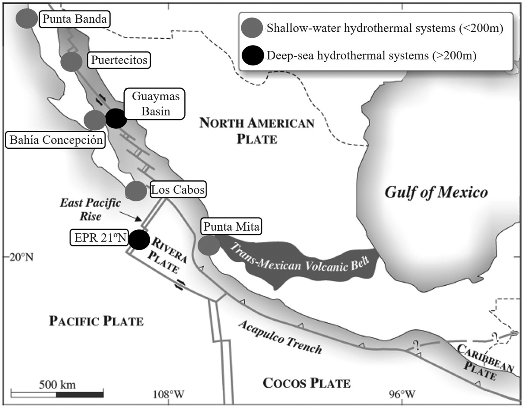
Fig. 1. Distribution of deep-sea and shallow-water hydrothermal systems in Mexico. Grey circles indicate shallow-water systems and black circles deep-sea ones. Modified map of Canet & Prol-Ledesma (Reference Canet and Prol-Ledesma2007).
In one of the five shallow-water hydrothermal systems in Mexico, in Bahía Concepción, in Baja California Sur, a study has been carried out on the benthic infauna that inhabits the sediments of this hydrothermal system (Melwani & Kim, Reference Melwani and Kim2008). This research focuses on the shallow-water hydrothermal system of Punta Mita (SWHSPM), located in Banderas Bay. This bay shares beaches of valuable tourist interest for the States of Nayarit and Jalisco, and the dominant ecosystem in this hydrothermal system has not yet been determined. Therefore, this research aims to characterize the distribution of the benthic infauna that coexist in the SWHSPM.
Materials and methods
Study area
The SWHSPM is located in the area of Fisura Las Coronas (Núñez-Cornú et al., Reference Núñez-Cornú, Prol-Ledesma, Cupul-Magaña and Suárez-Plascencia2000). Fernández de la Vega-Márquez & Prol-Ledesma (Reference Fernández de la Vega-Márquez and Prol-Ledesma2011) reported the main geological line-ups related to this fissure. These line-ups correspond to the extensional tectonism phase of the area, which is the most recent and the cause of the Puerto Vallarta graben (Fernández de la Vega-Márquez & Prol-Ledesma, Reference Fernández de la Vega-Márquez and Prol-Ledesma2011). The oceanic environment of Banderas Bay is influenced by four main ocean currents: the California current, North-equatorial current, reflux from the Gulf of California and coastal ocean current from Costa Rica (Prol-Ledesma et al., Reference Prol-Ledesma, Canet, Villanueva-Estrada and Ortega-Osorio2010). These currents bring arctic, subtropical and equatorial water to this bay.
In ~400 m of the beaches of Punta Pantoque in Banderas Bay, Nayarit, Mexico, at a depth of 9 m, three sites with hydrothermal activity (Figure 2) were selected: Site 1 (S1) (20°44′54.7″N 105°28′40.6″W), Site 2 (S2) (20°44′54.8″N 105°28′40.4″W) and Site 3 (S3) (20°44′54.9″N 105°28′38.4″W). These three sites were selected because they had some of the most prominent and well-formed hydrothermal vents, compared with other sites. The distance between S1 and S2 was ~7 m, between S2 and S3 ~58 m, and between S3 and S1 ~64 m.
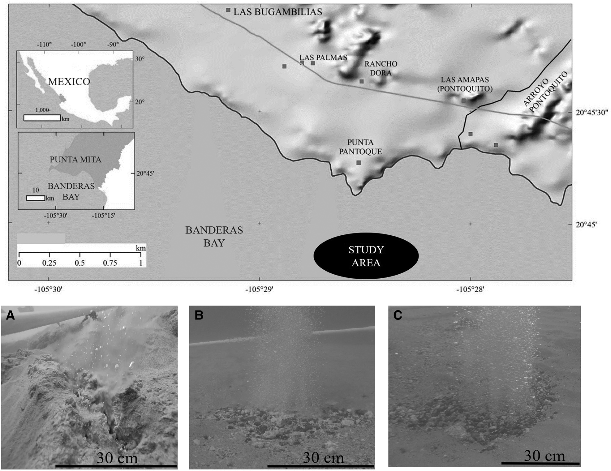
Fig. 2. Location of the study site. The black oval indicates the study area (modified from Rodríguez-Uribe et al., Reference Rodríguez-Uribe, Núñez-Cornú, Chávez-Dagostino and Trejo-Gómez2020). Pictures (A), (B) and (C) illustrate the main hydrothermal vents for each study site. (A) for site 1, (B) site 2 and (C) site 3.
Hydrothermal discharges in the SWHSPM originate mounds of calcareous tufa with Ba, Hg and Tl mineralization. These mounds are formed of finely laminated calcite aggregates, and on the surfaces of these they develop arborescent textures (Canet & Prol-Ledesma, Reference Canet and Prol-Ledesma2006). The basaltic rocks of the seabed, in the areas close to the fluid ascent ducts, are affected by hydrothermal alteration; altered basalts present plagioclase phenocrysts replaced by zeolites (heulandite and analcime) (Canet & Prol-Ledesma, Reference Canet and Prol-Ledesma2006).
The shallow depth of the SWHSPM determines the morphology and characteristics of the accumulations of hydrothermal precipitates, since the bottom is subject to the action of waves, storms and bottom currents, the waves preventing the formation of prominent mounds (Canet et al., Reference Canet, Prol-Ledesma and Melgarejo2000). In Figure 2A–C the main hydrothermal vents for each site are shown.
Sediment samples collection
Each study site was divided into three habitats (Figure 3), based on the bottom water temperature and the proximity to the mouth of each vent chimney. Habitat 1 (H1) is the closest to the discharge of hydrothermal fluids with an area of 0.16 m2; habitat 2 (H2) follows with 9 m2, and habitat 3 (H3) is the furthest from the hydrothermal influence with an area of 36 m2. In each habitat, a square area was considered. 10 × 10 cm PVC, 10 cm in diameter, plastic cores were used. On 23 November 2017, three sediment cores were collected by scuba diving in each habitat of each study site (N = 27), the approximate volume of each one was 785.40 cm3. The plastic core was inserted in the first 10 cm of the sediment or at a shallower depth if the substrate did not allow it. The 27 sediment samples were frozen at −20°C until processing, in an 11 ft Torrey® horizontal refrigerator.

Fig. 3. Diagram showing positions of the three habitats at each study site. The black circle represents the hydrothermal vent. (H1) habitat 1, (H2) habitat 2 and (H3) habitat 3.
Measurements of physicochemical parameters
To record the sediment temperature of each study site (0, 3, 5 and 10 cm), a TaylorTM analogue soil thermometer, 6099N model, 1″ diameter hood, 6″ stem was used, with a temperature range from −10 to 110°C. A YSITM Professional 1030 multiparameter probe (Pro1030) was used to record the pH, conductivity, salinity and seawater temperature at each study site.
Separation and taxonomic identification
The collected individuals were identified at the Marine Zoology Laboratory of the Instituto Tecnológico de Bahía de Banderas, Nayarit, Mexico. All the sediment cores (N = 27) were sieved in an 8″ ALCONTM brass sieve number 20 with a mesh size of 850 μm and later in a number 50 sieve of 300 μm. The individuals were fixed in 96% alcohol until identification. These individuals were observed using an Optika™ 50 × stereoscopic microscope (Via Rigla, Bergamo, Italy), and were identified to the class taxonomic level, through the literature of De León-González et al. (Reference De León-González, Bastida-Zavala, Carrera-Parra, García-Garza, Peña-Rivera, Salazar-Vallejo and Solis-Weiss2009) for polychaetes and Brusca et al. (Reference Brusca, Moore and Shuster2016) for the rest of the groups. The composition of the community was described with the indices of Shannon–Wiener's diversity (H′). Pielou's evenness (J′) and Simpson's dominance (λ) were also calculated (Zhou et al., Reference Zhou, Wang, Li and Bralts2017).
Organic matter content in sediment
The organic matter content was determined using the loss on ignition (LOI) method of Dean (Reference Dean1974), with 20 g of sediment taken from each sediment core (N = 27). An MMM™ stove, Incucell model, was used to remove humidity from samples, an Ohaus Scout™ precision balance, SPX2202 model, was used to weigh the samples, and a Thermolyne™ muffle, Furnace 48,000 model, where the treated samples were ignited at 550°C for 1 h.
Statistical analysis
A multivariate analysis of variance based on permutations (PERMANOVA) was applied in PRIMER™ + PERMANOVA version 6 software (Anderson et al., Reference Anderson, Gorley and Clarke2008) with two factors, sites, and habitats, nested habitats to sites, this with fixed effects (type I model), to determine if there is variation in abundance at the class level of the benthic infauna of the SWHSPM. As a measure of distance, the Sorensen index was used for the abundance data, which were previously transformed with fourth root (Downing, Reference Downing1979), to reduce the variation between the data, and 10,000 permutations were performed to test the statistical significance. The significance value was P ≤ 0.05 (Anderson, Reference Anderson2005).
PRIMER™ + PERMANOVA version 6 software (Anderson et al., Reference Anderson, Gorley and Clarke2008) was used to perform a principal coordinate analysis (PCO) (Gower, Reference Gower1966) with multiple correlations to associate the benthic infauna with the habitats and study sites. For this, the previous data matrix was used, and the similarity matrix was built with Euclidean distances.
For abiotic factors a PCO analysis was elaborated, previously a collinearity test was performed and only the most representative abiotic factors (pH, sediment temperature, water temperature, salinity and conductivity) were considered and those that explained the same as other factors were removed from the analysis. The data were normalized to Z values because they are factors of different nature (Legendre & Legendre, Reference Legendre and Legendre2012). After this, the similarity matrix with Euclidean distance was calculated.
Results
Benthic infauna
The number of individuals were 371, corresponding to eight classes: Malacostraca, Maxillopoda, Gastropoda, Bivalvia, Scaphopoda, Polychaeta, Leptocardii and Stenolaemata. The Malacostraca class was the most abundant in the three sites with 64.69% of the total abundance, followed by the Polychaeta class with 19.14% of the total. Figure 4 shows some representative individuals for each group. At S2 the highest abundance was found (58.22%), followed by S3 (30.73%) and S1 had the lowest (11.05%). The highest class richness was found in S3 and the lowest in S2 (Figure 5 and Table 1).
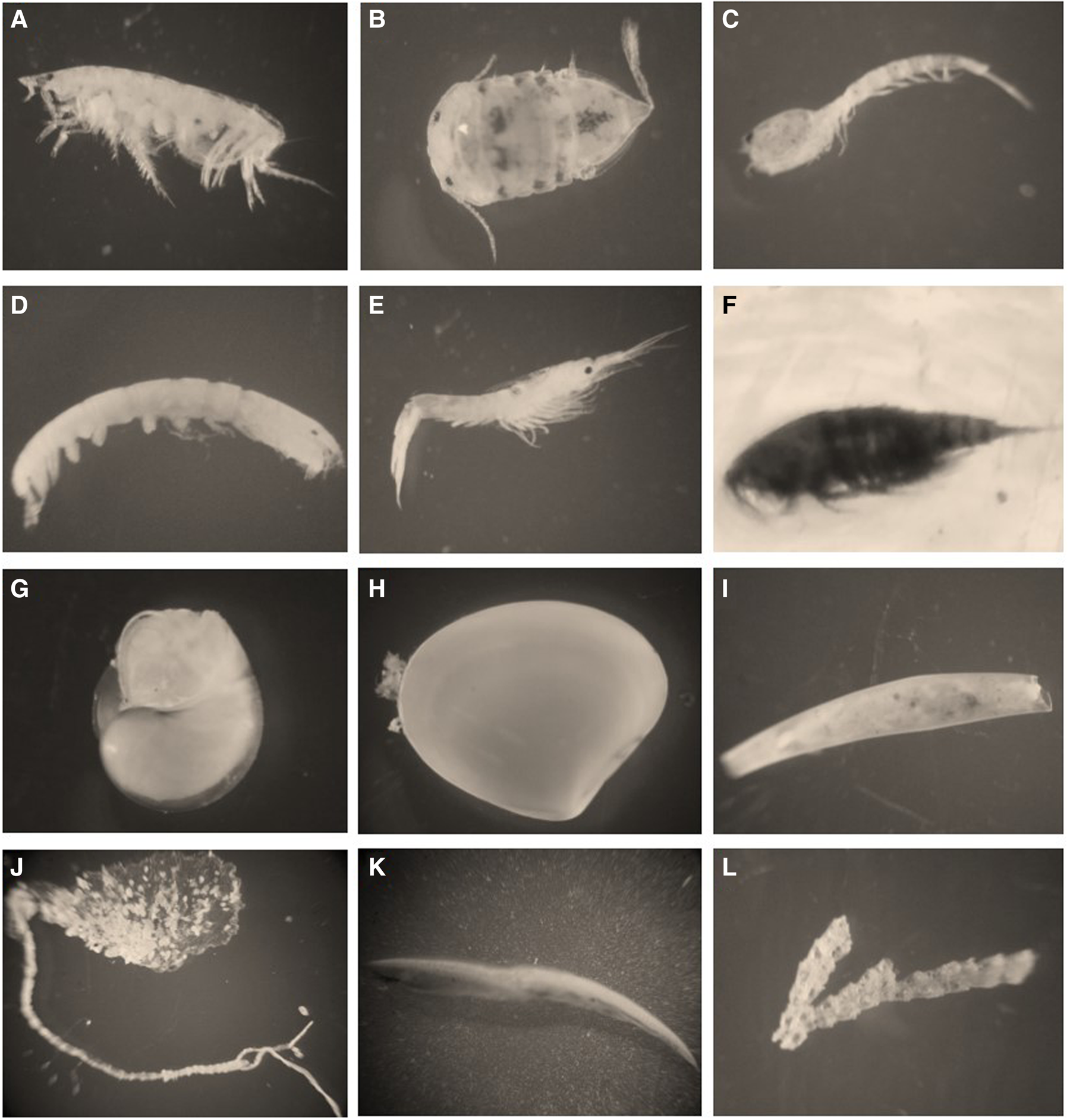
Fig. 4. Photographs of the representative individuals of each group in each taxonomic class: (A) Amphipods (Malacostraca); (B) Isopods (Malacostraca); (C) Cumaceans (Malacostraca); (D) Tanaidaceans (Malacostraca); (E) Decapods (Malacostraca); (F) Copepods (Maxillopoda); (G) Gastropods (Gastropoda); (H) Bivalves (Bivalvia); (I) Scaphopods (Scaphopoda); (J) Polychaetes (Polychaeta); (K) Amphioxus (Leptocardii); (L) Bryozoans (Stenolaemata C).

Fig. 5. Benthic infaunal total abundance at each study site indicated by the grey bars, and the total class richness is indicated by the black bars. The x-axis indicates the study sites (site 1, S1; site 2, S2; site 3, S3), and the y-axis indicates on the left side the abundance in the number of individuals, while on the right side indicates the total class richness per site.
Table 1. Benthic infaunal total abundance, and richness at the taxonomic class level, of the three study sites. Site 1 (S1), site 2 (S2), and site 3 (S3)

The Olmstead–Tukey diagram (Figure 6) shows that the Malacostraca and Polychaeta are dominant, Gastropoda and Maxillopoda are frequent, while rare classes are Leptocardii, Scaphopoda, Stenolaemata and Bivalvia.

Fig. 6. Olmstead–Tukey diagram. This diagram indicates that the Malacostraca and Polychaeta classes are the dominant ones in this research, while Scaphopoda, Leptocardii, Stenolaemata and Bivalvia are the rare ones. The x-axis shows the frequency of the classes in percentage, and the y-axis is the abundance in number of individuals (transformed with a square root). Black dots locate each class on the diagram.
In each study site, H1, which is the habitat directly affected by hydrothermal activity, presents the lowest abundance values in the three sites, while the highest values were in H2 (Tables 2 and 3).
Table 2. The number of individuals per habitat of each study site, with their respective abundance in percentage

Site 1 (S1), site 2 (S2), site 3 (S3), habitat 1 (H1), habitat 2 (H2) and habitat 3 (H3).
Table 3. Benthic infaunal total abundance of the three study habitats, and richness at the taxonomic class level

The results of the PERMANOVA analysis indicated that the number of individuals were significantly different between sites ( P = 0.0025), while the abundance also differed between habitats and sites ( P = 0.0089). The paired posteriori tests determined that the means of the three sites are different, S1 being different from S2 ( P = 0.0123), S1 different from S3 (P = 0.0403) and S2 different from S3 ( P = 0.0056); regarding the habitats, H1 is different from H3 (P = 0.0017) and there were no significant differences between H1 and H2, nor between H2 and H3 (Figure 7).

Fig. 7. Benthic infaunal abundance by the habitat of each study site. Black bars indicate the abundance of site 1 (S1), the light grey bars of site 2 (S2), and the dark grey ones of site 3 (S3). The uppercase letters above the bars indicate significant differences between the study sites, while lowercase letters indicate significant differences between habitats at each site. Habitat 1 (H1), habitat 2 (H2) and habitat 3 (H3).
The ecological indices for this community (Table 4) shown that the value of H′ was higher in S3, and S2 presented the lowest value. Meanwhile, the highest value of J′ was presented at S1 and S2, and the lowest at S3. Concerning the values of λ, they had the same behaviour as the J′ values.
Table 4. Ecological indices

Site 1 (S1), site 2 (S2), and site 3 (S3), Shannon–Wiener's diversity index (H′), Pielou's evenness index (J′) and Simpson's dominance index (λ).
Table 5 shows the ecological indices of the community of each habitat at each study site. In S1, it is observed that the highest value of H′ was in H2 and the lowest in H1, concerning J′ the highest value was in H3 and the lowest in H1, meanwhile the highest value of λ was in H1 and the lowest in H3. In S2, it is observed that the highest value of H′ was in H1 and the lowest in H3, concerning J′ the highest value was in H1 and the lowest in H3, meanwhile the highest value of λ was in H2 and the lowest in H1. In S3, it is observed that the highest value of H′ was in H1 and the lowest in H3, concerning J′ the highest value was in H1 and the lowest in H3, meanwhile the highest value of λ was in H3 and the lowest in H1.
Table 5. Ecological indices of each habitat in the three study sites

Shannon-Wiener's diversity (H′), Pielou's evenness (J′) and Simpson's dominance (λ), habitat 1 (H1), habitat 2 (H2), and habitat 3 (H3).
The galleries are tubes where benthic fauna are protected or hidden; 226 galleries were found of vermetids, polychaetes and tanaidaceans. The largest number of galleries were in H1 of the three study sites, with 139 galleries, meanwhile H2 had 56 galleries and H3 had 31 galleries. Figure 8 shows pictures of three representative galleries, of those found at sampling sites.

Fig. 8. Photographs of the most representative galleries of those found in the three study sites: (A) gallery found in H1 of S1, (B) gallery found in H1 of S2 and (C) gallery found in H1 of S3.
Physicochemical parameters
Table 6 shows the sediment temperature records at different depths (0, 3, 5 and 10 cm) in each habitat by study site. H1 in the three study sites recorded the highest temperatures, which increased as the depth of the sediment increased, meanwhile H3 presented the lowest values.
Table 6. Temperatures in °C of different depths (0, 3, 5 and 10 cm) of the sediment in each habitat of each study site

Recorded on 23 November 2017. Habitat 1 (H1), habitat 2 (H2), habitat 3 (H3), site 1 (S1), site 2 (S2) and site 3 (S3).
Four physicochemical parameters (pH, conductivity, salinity and temperature) in each habitat of each study site were recorded on two different dates (on 23 November 2017 and 4 June 2018). This was in order to observe these parameters in a cold season (November) and in a warm season (June). These parameters were recorded from 10:00–14:00 h, the means and the standard error are shown in Table 7.
Table 7. Physicochemical parameters in each habitat of each study site (N = 72)

Data were recorded on 23 November 2017 and 4 June 2018. Habitat 1 (H1), habitat 2 (H2), habitat 3 (H3), site 1 (S1), site 2 (S2) and site 3 (S3).
In Table 7, it is observed that there is an inverse relationship concerning temperature and the rest of the parameters (pH, conductivity and salinity), that is, the higher the temperature, the lower pH, conductivity and salinity; this was observed at all three study sites. Meanwhile, H1 of the three sites recorded the highest temperatures, having a greater difference of up to 60°C with respect to H3, which is the habitat without the influence of hydrothermal activity.
Organic matter
The average organic matter content found in the sediment samples for each habitat at each study site is shown in Table 8. The H3 of the three sites presented on average the lowest organic matter content (0.35 ± 0.012 g), meanwhile, H1 of the three sites presented on average the highest organic matter content (0.41 ± 0.035 g). Specifically, H1 of the S3 presented the highest content (0.048 ± 0.003 g).
Table 8. Organic matter contained in the sediment samples by the habitat of each study site

The average content is shown with its respective standard error. From the samples collected on 23 November 2017. Habitat 1 (H1), habitat 2 (H2), habitat 3 (H3), site 1 (S1), site 2 (S2) and site 3 (S3).
Relationship of the benthic infauna with environmental parameters
The principal coordinate analysis (PCO) at the class level (Figure 9) presents an explained variation of 67.9%, in the first two axes; 38% of this variation is explained in the first axis (PCO1), while 29.9% in the second (PCO2). The explained variation in this analysis suggests the existence of an affinity of the taxonomic classes with respect to the study sites. That is, there are differences in the classes present in the study sites, which are observed in S1 and S2 concerning S3. Meanwhile, S1 and S2 are located mostly in the positive values, S3 disperses from the negative to the positive values of the first axis. Specifically, Maxillopoda, Malacostraca, Polychaeta, Bivalvia, Stenolaemata, Scaphopoda and Leptocardi classes show an affinity for S3, except the Gastropoda class. And the Stenolaemata, Scaphopoda and Leptocardi classes do not show an affinity for S1 and S2.

Fig. 9. Principal coordinate analysis graph. Grey triangles indicate H1, black triangles H2, grey squares H3, and the classes are labelled with their name. The x-axis explains 38% of the total variation and the y-axis explains 29.9%. Habitat 1 (H1), habitat 2 (H2), habitat 3 (H3), site 1 (S1), site 2 (S2) and site 3 (S3).
The PCO of environmental factors (Figure 10) presents an explained variation of 99.1% in the two first axes, where PCO1 contains 97.9% of this variation and PCO2 1.2%. This suggests an affinity of the habitat types to the environmental factors. In other words, three groups are visibly grouped, group 1: the three H1 of the three sites, group 2: the three H2 of the three sites, and group 3: the three H3 of the three sites. Besides, an inverse relationship is also observed between the water temperature and the sediment temperature, with respect to the conductivity, salinity and pH. In particular, it is observed that H1 of the three sites correlates with the highest water and sediment temperatures, H2 with intermediate values of the five environmental factors analysed, while H3 of the three sites with the lowest water and sediment temperatures, and with the highest amounts of conductivity, salinity and pH.

Fig. 10. Principal coordinate analysis graph. Grey triangles indicate H1, black triangles H2, grey squares H3, and the environmental factors are labelled with their name. The x-axis explains 97.9% of the total variation and the y-axis explains 1.2%. Habitat 1 (H1), habitat 2 (H2), habitat 3 (H3), site 1 (S1), site 2 (S2) and site 3 (S3).
In Figures 9 and 10, it can be seen that the eight taxonomic classes have a greater affinity for H2 and H3 habitats at all three study sites, which are related to the lower temperatures of both the water and the sediment, as well as higher conductivity, salinity and pH measurements.
Discussion
The area of direct hydrothermal influence, called H1 of the three study sites in the SWHSPM presented the highest temperatures, both in the water and in the sediment, as well as the lowest values of pH, conductivity and salinity (these characteristics indicate the highest proportion of thermal water in the discharge and coincide with the calculated composition of the thermal end member that has high temperature, and a higher proportion of meteoric-origin water with lower salinity). This habitat has the lowest abundance of individuals and the highest abundance of galleries. Melwani & Kim (Reference Melwani and Kim2008) reported that the high temperatures in the shallow submarine hydrothermal system of Bahía Concepción, Mexico, excluded most of the species of infauna present in the zones adjacent to this hydrothermal system. They concluded that the hydrothermal influence zone and the transition zone housed species that have strategies to manage the effect of the high temperatures present in this system, which range from 50–90°C. The aforementioned agrees with what Kamenev et al. (Reference Kamenev, Fadeev, Selin, Tarasov and Malakhov1993), Dando et al. (Reference Dando, Hughes, Leahy, Niven, Taylor and Smith1995) and Tarasov et al. (Reference Tarasov, Gebruk, Shulkin, Kamenev, Fadeev, Kosmynin, Malakhov, Starynin and Obzhirov1999) reported, in that the macrofauna that inhabits the vicinity of a shallow hydrothermal influence must have certain types of protection from stressful physical conditions, in this case galleries.
The presence of galleries in the SWHSPM (vermetids, polychaetes and tanaidaceans) in all the habitats of the three sites makes it clear that benthic infauna has protection mechanisms against the hydrothermal influence of this hydrothermal system. We found that the highest abundances of galleries were found in H1 of the three sites, and this abundance decreased with increasing distance from the hydrothermal influence. Morri et al. (Reference Morri, Blanchi, Cocito, Peirano, De Biase, Aliani, Pansini, Boyer, Ferdeghini, Pestarino and Dando1999) suggested that the complexity generated by tubes and shells is a characteristic of fauna that inhabit shallow-water hydrothermal systems. Also, Chevaldonne et al. (Reference Chevaldonne, Desbruyeres and Childress1992) highlight that the use of tubes, shells and other calcareous remains can allow many species to survive the temperature differences around hydrothermal systems. The fact that the individuals of the benthic infauna in this study site build tubes or galleries may be a behavioural mechanism rather than a detoxification action for surviving in a habitat with hydrothermal activity (Gamenick et al., Reference Gamenick, Jahn, Vopel and Giere1996).
In this research we are reporting that the Malacostraca and Polychaeta were the dominant classes, where the Malacostraca class includes microcrustaceans, amphipods, isopods, cumaceans, tanaidaceans and copepods. Both classes were present in the three habitats of the three study sites; these individuals have higher mobility, compared with the classes that turned out to be the rarest, i.e. Scaphopoda, Stenolaemata, Leptocardii and Bivalvia, which includes individuals with low mobility. According to Melwani & Kim (Reference Melwani and Kim2008), mobility in species that inhabit submarine hydrothermal systems provides them with a strategy for survival when protection, tolerance or detoxification mechanisms are absent. Although swimmers have a more mobile strategy, other sediment-dwelling groups can also exploit mobility, either burrowing or crawling. The textural composition of the sediments of S1, S2 and S3 has been reported by Rodríguez-Uribe et al. (Reference Rodríguez-Uribe, Núñez-Cornú, Chávez-Dagostino and Trejo-Gómez2020), ~2 weeks apart, they collected the samples on 13 December 2017, where the very fine sand was the dominant grain size in the three sites.
The presence of the Leptocardii class was not recorded in any hydrothermal influence area. This class includes the cephalochordates; the adults are occasional swimmers since they prefer the benthic substrate for the locomotion, where they spend most of their time filtering their food (Garcia-Fernàndez & Benito-Gutiérrez, Reference Garcia-Fernàndez and Benito-Gutiérrez2009). Most probably the absence of these is due to the high temperatures of the sediment, since cephalochordates generally inhabit shallow marine waters near the coast (Del Moral-Flores et al., Reference Del Moral-Flores, Guadarrama-Martínez and Flores-Coto2016; Galván-Villa et al., Reference Galván-Villa, Ríos-Jara and Ayón-Parente2017).
The three H1 of the three study sites presented the lowest abundances of individuals and a benthic infauna community very similar to that found in the habitats farthest from the hydrothermal influence (H2 and H3), except for the Leptocardii class. This result is attributed to the stressful conditions of the habitat with the direct hydrothermal influence of the SWHSPM. Couto et al. (Reference Couto, Rodrigues and Neto2015) carried out a review of the papers on flora and fauna present in shallow-water hydrothermal systems in the Azores Islands in Portugal, and found that the individuals within these hydrothermal systems are similar to those found in the coastal and submarine areas of the archipelago (Cardigos et al., Reference Cardigos, Colaço, Dando, Ávila, Sarradin, Tempera, Conceição, Pascoal and Santos2005), but with lower abundances. Also, in the comparative study of Marques-Mendes (Reference Marques-Mendes2008) between the benthos communities affected by hydrothermal activity and another site without this activity, he concludes that the community present in the hydrothermal system has almost the same composition as the communities without hydrothermal activity, but with less abundance.
Hall-Spencer et al. (Reference Hall-Spencer, Rodolfo-Metalpa, Martin, Ransome, Fine, Turner, Rowley, Tedesco and Buia2008) reported how acidification caused by gas discharges in cold vent areas off Ischia in Italy significantly decreased the abundances of certain species of coralline algae, where the pH levels recorded were the lowest in the study (7.4–7.5). On the other hand, in the study of Álvarez-Castillo et al. (Reference Álvarez-Castillo, Hermoso-Salazar, Estradas-Romero, Rivas and Prol-Ledesma2018) carried out in the Wagner and Consag basins, Gulf of California, Mexico, where more than 300 sites with CO2 bubbles rising to the surface have been reported, they reported that lower meiofauna densities were also related to lower pH levels (6.06–6.48). The aforementioned is in agreement with our results since the lowest pH levels (7.64–7.74) were recorded in the areas of direct influence of the SWHSPM, which has been associated with a lower abundance of infauna in those study areas.
Quite contrary to the chemical conditions in SWHSPM, in sulphurous hydrothermal systems, the abundances of polychaetes are often increased, due to the high tolerance to hydrogen sulphide and anoxia (Melwani & Kim, Reference Melwani and Kim2008). Thus, in White Point hydrothermal vents (San Pedro Bay, USA) hydrogen sulphide was the most influential variable between the zones with and without hydrothermal activity, therefore the polychaetes Apoprionospio pygmaea and Prionospio heterobranchia, both of the family Spionidae were the most abundant in this site (Melwani & Kim, Reference Melwani and Kim2008). Nereid and capitellid polychaetes have already been documented to be able to tolerate long-term sulphide exposure (Vismann, Reference Vismann1990). The sulphidic habitats have been proposed as ideal refuges for animals capable of resisting sulphide toxicity (Bagarinao, Reference Bagarinao1992). It has also been reported that certain genera of algae have been shown to be resistant to natural amounts of pCO2 (Hall-Spencer et al., Reference Hall-Spencer, Rodolfo-Metalpa, Martin, Ransome, Fine, Turner, Rowley, Tedesco and Buia2008), for example, Caulerpa, Cladophora, Asparagopsis, Dictyota and Sargassum, and that they are directly related to low pH levels as reported in the cold vent areas off Ischia in Italy (Hall-Spencer et al., Reference Hall-Spencer, Rodolfo-Metalpa, Martin, Ransome, Fine, Turner, Rowley, Tedesco and Buia2008). Some of these algal species include invasive alien species that have already begun to alter shallow marine ecosystems worldwide (Boudouresque & Verlaque, Reference Boudouresque and Verlaque2002; Hall-Spencer et al., Reference Hall-Spencer, Rodolfo-Metalpa, Martin, Ransome, Fine, Turner, Rowley, Tedesco and Buia2008).
The high temperature (89°C) of the SWHSPM has an inverse relationship with pH and salinity, thus being the environmental factor that structures the benthic infaunal community, since it was the only environmental variable that differed significantly between the three habitats of the three study sites. Despite this, members of the communities adjacent to this hydrothermal system are not completely excluded, since the only class that does not occur in the area of hydrothermal influence is the Leptocardii, because they do not tolerate high sediment temperatures, while the remaining seven classes are present, only in lower abundances. In addition, the benthic individuals present in the hydrothermal influence area use protection strategies against extreme conditions, evidenced by the high abundance of galleries found in this habitat. The temperature and pH levels in the SWHSPM make this site a place with great potential for the study of ocean acidification, due to its shallow depth and proximity to the beach.
Acknowledgements
We thank Natalia Balzareti Merino for the coordination of diving activities, sampling and photography work (see Figure 2A–C). To Amilcar L. Cupul Magaña for the advice in the samples process and organic matter method. And a very special thanks to Rosa María Chávez Dagostino for all the advice, accompaniment and help in this research.
Author contributions
MCRU carried out the study, and conducted the compilation, analysis of the research, and drafted the manuscript. FJNC participated in the designed the study, acquired the financial support, and revised and edited the manuscript. RMPL participated in the design of the study, interpretation of the findings, and revised and edited the manuscript. PSS validated the taxonomic classification. All authors read and approved the final manuscript.
Financial support
This research was funded by Centro Mexicano de Innovación en Energía-Geotérmica (CeMIE-Geo). P24. Passive and magnetotelluric seismic exploration in the geothermal fields of La Caldera of La Primavera and Ceboruco Volcano, SENER-CONACyT 201301-207032.


