


Introduction
The first cases of community coronavirus 2019 (Covid-19) transmission in the United States were reported in California, Oregon, Washington state and New York state in late February 2020 [Reference Schumaker1]. A Santa Clara, California death on 6 February was deemed the country's first Covid-19 fatality after an autopsy was conducted in April [Reference Schumaker1]. A national emergency was declared by US President Donald Trump on 13 March 2020, and testing several days later revealed that Covid-19 had spread to all 50 states [Reference Schumaker1]. On 20 March, New York City was declared the US outbreak epicentre [Reference Schumaker1]. A study, released in April 2020 as a preprint, found via genetic analysis of Covid-19 cases in New York City that the majority of the viruses originated in Europe – revealing that transmissions had begun as early as January from countries with no travel monitoring [Reference Gonzalez-Reiche2]. As of 29 June 2020, the US had 2 496 628 confirmed Covid-19 cases, and 125 318 Covid-19 deaths [3].
Covid-19 challenges faced by the US include fair allocation of adequate medical resources [Reference Emanuel4], minimising mortality, avoiding overwhelming the health-care system and keeping the effects of lockdown policies on the economy within manageable levels [Reference Anderson5]. Epidemiological analysis of the virus proliferation is needed to assess the impacts of mitigation strategies including social distancing, sheltering-in-place (voluntary) and quarantines (enforced by authorities) [Reference Anderson5], as well as personal habits including frequent hand washing and wearing masks. We have developed a new compartmental model, extending the long-standing SIR (Susceptible, Infected, Removed) model [Reference Brauer, Castillo-Chavez and Feng6–Reference Chang8], to evaluate and compare several states' responses to Covid-19; with this model we can make estimates, using curve fitting of reported data, of the impact of contact suppression measures and the lifting of such measures. We find that, for the current situation where several states have relaxed stay-at-home measures, Covid-19 will become an endemic virus for at least two years; so it is not surprising that some states are reinstating the stay-at-home measures [Reference Lee9]. More in-depth projections (made by varying contact rates, detection rates and sequestration adherence), using Texas as a test case, suggest that a modest increase in the testing rate, a modest decrease in the contact rate or a significant increase in lockdown compliance could eradicate the virus within a year.
A new model
Our SQUIDER model incorporates additional processes into the classic SIR model: (i) making a distinction between known cases (which are publicly reported) and asymptomatic or mild cases which are not monitored or detected; (ii) including the effects of responses, with varying adherence by region, to the pandemic, whether direct, through quarantine or medical isolation of diagnosed cases, or less direct such as social distancing efforts and (iii) possible loss of immunity of recovered individuals, allowing some of them to be reintroduced into the Susceptible population. The model thus requires several new compartments, which we will denote as U (Undetected infected), E (undetected recovered) and Q (pseudo-Quarantine, a bin to hold a segment of the susceptible and undetected infected populations allowing us to model reduced human interactions due to social distancing). Furthermore, for modelling/fitting purposes we add a separate compartment D for known infecteds who die; while undetected infections, undetected deaths, undetected recoveries and quarantine adherence are not available, deaths from the virus are generally reported [10]. Figure 1 shows the connections among different compartments in our model.

Fig. 1. Schematic of the compartments, with the rates of transfer between the compartments.
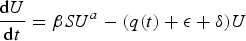
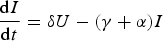
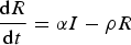
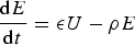
The rate equations are as follows:


Each compartment is normalised by the total population N; hence

Note that the coefficients α, β, δ, ε, γ and ρ are constants (to be evaluated from fits to data). Being normalised, our compartment variables are non-dimensional, and our rate coefficients have units of days to the power of −1, so the model could be described as a one-dimensional continuous dynamical system.
Before we go through the individual equations we should discuss some of the recurring terms and factors. First, the incidence rate βSUa, the average normalised new infections in time, is nonlinear when a ≠ 1. Here β is the contact rate, which is the average number of contacts a person has per day, multiplied by the probability of transmitting the disease when contact between a Susceptible and an Undetected infected occurs, i.e. the level of contagiousness. Detected Infecteds (I) are not involved since we assume that, post-diagnosis, the I group are generally in medical isolation or some other form of quarantine [Reference Parmet and Sinha11]. If a = 1, this term describes homogenous mixing of the Susceptible and Undetected infected populations [Reference Liu and Stechlinski12], which may not be accurate for states with isolated populations, low population densities, or many densely populated areas; the relationship may be sublinear or superlinear depending on the population being sparse or dense. Power law incidence rates (such as βSUa) have been shown to improve the accuracy of SIR models [Reference Novozhilov13, Reference Roy and Pascual14].
Second, the factor q(t) models the time dependence of social distancing and contact suppression, as well as the effects of subsequent lockdown release. Social distancing is modelled by transferring a proportion of the Susceptible and Undetetected infected populations at a time t 1 into the Q compartment. This does not imply that some large number of undiagnosed people are put into any actual physical quarantine, only that the available sub-groups for infecting (U) and for becoming infected (S) are reduced; alternatively, this might possibly be modelled by altering β or the power law dependency a in a time-dependent way. Mathematically, this transfer is realised within the ODE model by having q(t) be time-dependent – that is 0 until close to the time of sequestration; it then becomes large very quickly and then subsides quickly to 0 again; in other words, q(t) is a pulse. This pulse transfers populations between compartments – for example, from S and U to Q at the start of a lockdown, and from Q to S when lockdown is released. Note that the transferred population will stay in the Q compartment until a subsequent, negatively weighted q 2(t) pulse is generated. This pulse form was chosen, as opposed to a constant value used by some authors [Reference Xu15–Reference Maier and Brockmann17], because many states went into lockdown on a particular day with some, but not all, people self-isolating [Reference Gostin, Hodge and Wiley18, Reference Mervosh, Lu and Swales19]. In particular, the day t 1 where such measures take effect and the maximum pulse magnitude q 1 are of interest because they reflect the compliance (or lack thereof) of the state's population. A constant rate of sequestration, on the other hand, is not only somewhat unnatural in terms of social dynamics, but will result in the entire population eventually being sequestered unless there is some opposite movement taking people out of sequestration as well.
Equation 1 for the Susceptible population is reduced nonlinearly by new infections βSUa due to interactions, and explicitly reduced in a time-dependent way by sequestration q(t)S (not by any significant amount until we get close to the activation time t 1), as well as increased again by re-entrance at a rate ρ by the undetected recovered (E) and Recovered (R) groups. This term was added due to the WHO revelation that recovered Covid-19 patients may have little or waning immunity after exposure [20], later confirmed by an antibody study conducted on individuals who had recovered from Covid-19 infections [Reference Long21].
Equation 2, for Undetected infecteds, includes the increase due to contact with S members, and removal by various causes. The rate ε corresponds to the recovery rate in the basic SIR model. The detection rate δ specifies the proportion of Undetected infected individuals who are diagnosed with the virus (and are hence no longer undetected); it is added to the I compartment. Finally, this population is also effectively reduced due to social distancing q(t), e.g. residents of many states were encouraged to shelter at home and not seek testing/diagnosis unless they became symptomatic, in order to ease pressure on medical resources [22].
Equation 3 for the detected Infected population, describes increases due to testing at rate δ and decreases due to death with rate γ, and recovery with rate α. Since these individuals are isolated in designated hospital wards or under quarantine at home [Reference Parmet and Sinha11], hence unlikely to be a source of infection to the community at large, we felt there was no need for sequestration (i.e. q(t)) when social distancing went into effect. This is in agreement with the WHO guidance on quarantines segregating suspected exposed people [20].
Equation 4 describes the growth of detected Recovered, balanced by outflux of the Recovered population into the susceptible compartment at rate ρ due to little or waning immunity, expected for human coronaviruses [Reference Callow23]. Equation 5 describes the increase in Deceased detected individuals. Equation 6 describes the increase in the pseudo-Quarantine compartment due to official contact suppression measures q(t), which as stated above is only significant around the activation times t 1 and t 2. Equation 7 describes increases in the undetected recovered population at rate ε, and decreases in this population due to loss of immunity of E at rate ρ.
Assumptions
Several simplifying assumptions or idealisations have been made. To begin with, in our model the detected Infecteds (I) do not transmit the disease to the Susceptible (S) population. It is generally the case that in all such disease outbreaks (e.g. the 2014–2016 Ebola outbreak), even when strict quarantine measures are in place, medical service providers and other people rendering direct aid to victims are themselves vulnerable to infection; when the outbreak (in the non-healthcare worker population) is contained they may even make up the substantial proportion of cases [24]. However, in the current situation where the disease circulates through the general population and safety protocols are rigorously enforced by frontline health providers [Reference Ng25], the proportion of such cases relative to the general population is negligible.
Other simplifying assumptions: as mentioned above, we have opted to keep our contact rate β constant and instead vary the S and U compartment population levels to mimic social distancing effects (for example staying at home). In future versions of our model we may incorporate time-dependent β or a in order to disentangle population-wide transmission suppression (e.g. face masks and other protective gear for the public) from social contact suppression (cancellation of concerts and other public gatherings), but for the sake of simplicity in both coding and analysis we have opted for now to use only one time-dependent rate. In the same vein, the q(t) function removes Susceptibles and Undetected infecteds at the same rate (we have no reason at this time to differentiate the rates of change of these populations).
Similarly, people from the E and R compartments lose immunity at the same rate ρ. Indeed, it is possible that people who experienced milder forms of the disease (E) lose immunity faster than those who experienced more severe symptoms and sought out treatment (R) [Reference Long21]; however, we use a single rate ρ for simplicity. As other authors [Reference Moghadas16, Reference Kennedy26, Reference Li27], we did not consider our undetected recovery rate ε to be equivalent to α since it is possible that recovery rates are different for people with mild or no symptoms who do not seek medical care in comparison with people who do seek medical care (the I population). We additionally do not expect such mild or asymptomatic cases to be fatal [Reference Basu28]; therefore, people are not removed from the U compartment due to death. Note that, at least in the early days of the pandemic, increased overall deaths in comparison with the prior three years were not examined for signs that the virus was active among undiagnosed populations [Reference Weinberger29]. Finally, we do not consider the effects of births, vertical transmissions, immigrants, emigrants or deaths due to other diseases or trauma. The inclusion of deaths due to diagnosed virus cases makes the model not entirely static, but the disease's total deaths as a proportion of the total population is low enough that births and other such aspects can be safely omitted.
Results
Coefficient evaluation
Figure 2 shows fits of the model to data (cumulative confirmed case counts and deaths due to Covid-19) for Arizona, California, Florida, Illinois, Louisiana, New Jersey, New York State and Texas. The fits to cumulative case counts are all excellent – even for states such as Illinois, New Jersey and New York that have a distinct inflection in case counts. It is also apparent that some states, such as Arizona, California, Florida, Louisiana and Texas, have had rapidly rising case counts in June – likely due to easing of restrictions. This feature is captured by our q(t) – where application of a second, possibly negative pulse moves people from the Q to the S compartments as described above. Note that model fits to cumulative death counts deviate from the data starting in mid-May in some states (Arizona, California, Florida, Louisiana, New Jersey, New York and Texas). This may be due to improved medical treatments (such as dexamethasone [Reference Cain and Cidlowski30]), virus mutations resulting in a less deadly strain, or the postulated lack of reliability in confirmation of US Covid-19 deaths, which may be significantly undercounted [Reference Bump31]. Fit parameters are listed in Table 1. The contact and exclusion rates vary by less than 5%; however, reintroduction rate varies by 320%, detected recovery rate by 65%, re-release rate by 268%, stay-at-home effect by 103% and death rate by 59%. These variations, though large, are not surprising due to different states having been in different stages of the outbreak. For example, New York's and New Jersey's recovery rates are significantly lower than other states'. This could be due to the fact that these states had saturated hospital capacities during their peak outbreak [Reference Rothfield32, Reference Duffy33], causing slower recoveries due to decreased access to medical staff and treatments. Figure 3 additionally shows the dynamics of the U, E and R, as well as I and D (fitted compartments) over the fit period (22 January to 29 June 2020). Note that the U curves follow the I curves because individuals are transferred from U to I at a constant rate δ and out of I at a constant rate α + γ. In this figure, it appears that U and E cases in New York and New Jersey have stabilised, similar to the I + R cases in Figure 2. Presumably this is due to the outbreak occurring earlier in those states, and possibly because the official response has been more rigorous.
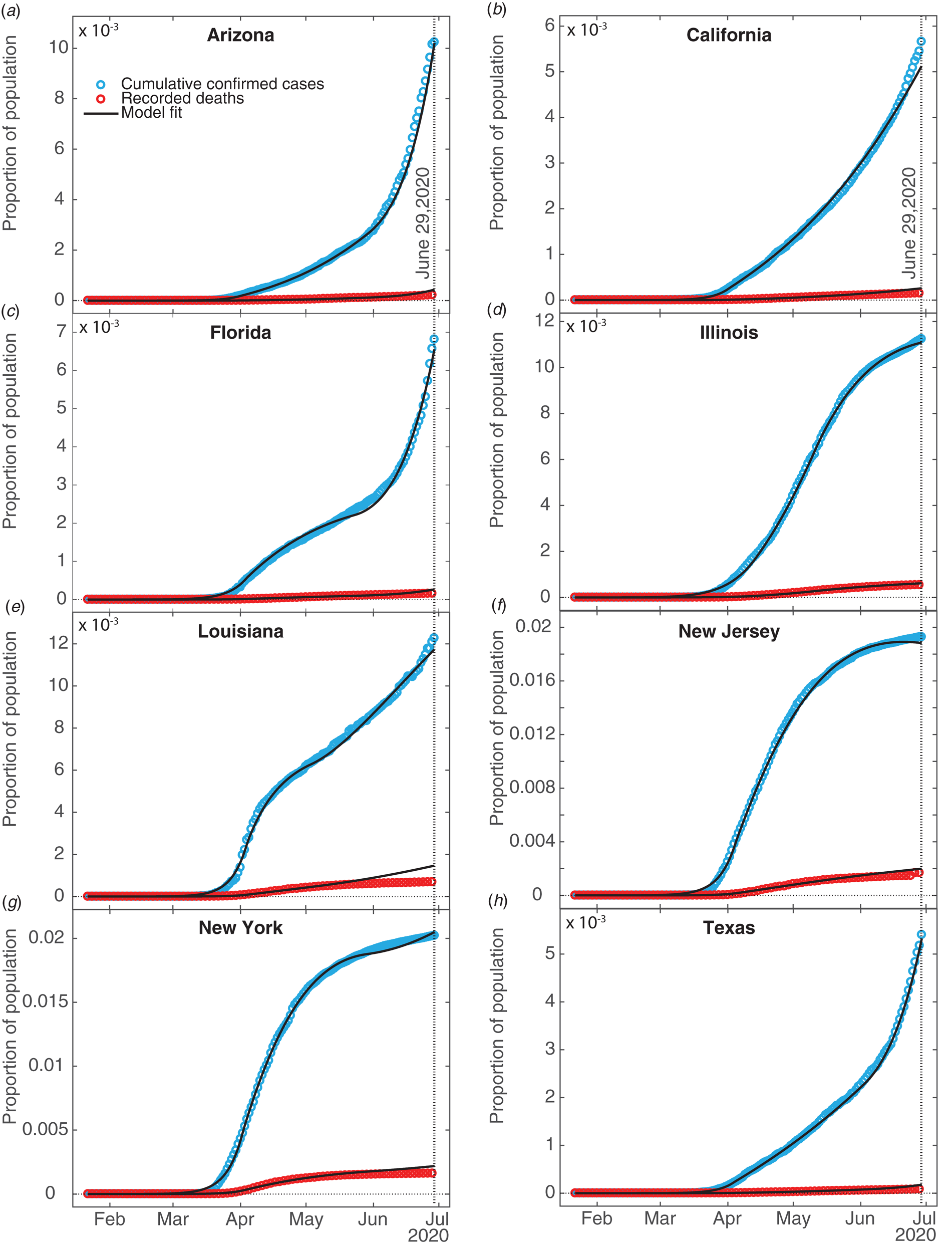
Fig. 2. SQUIDER model fits. Fits of our compartment model to recorded data on confirmed cumulative case counts and deaths; all fits have R 2 ≥ 0.996. Data were obtained from The Johns Hopkins University [34]. The vertical dotted line indicates the last date fitting data was obtained for.
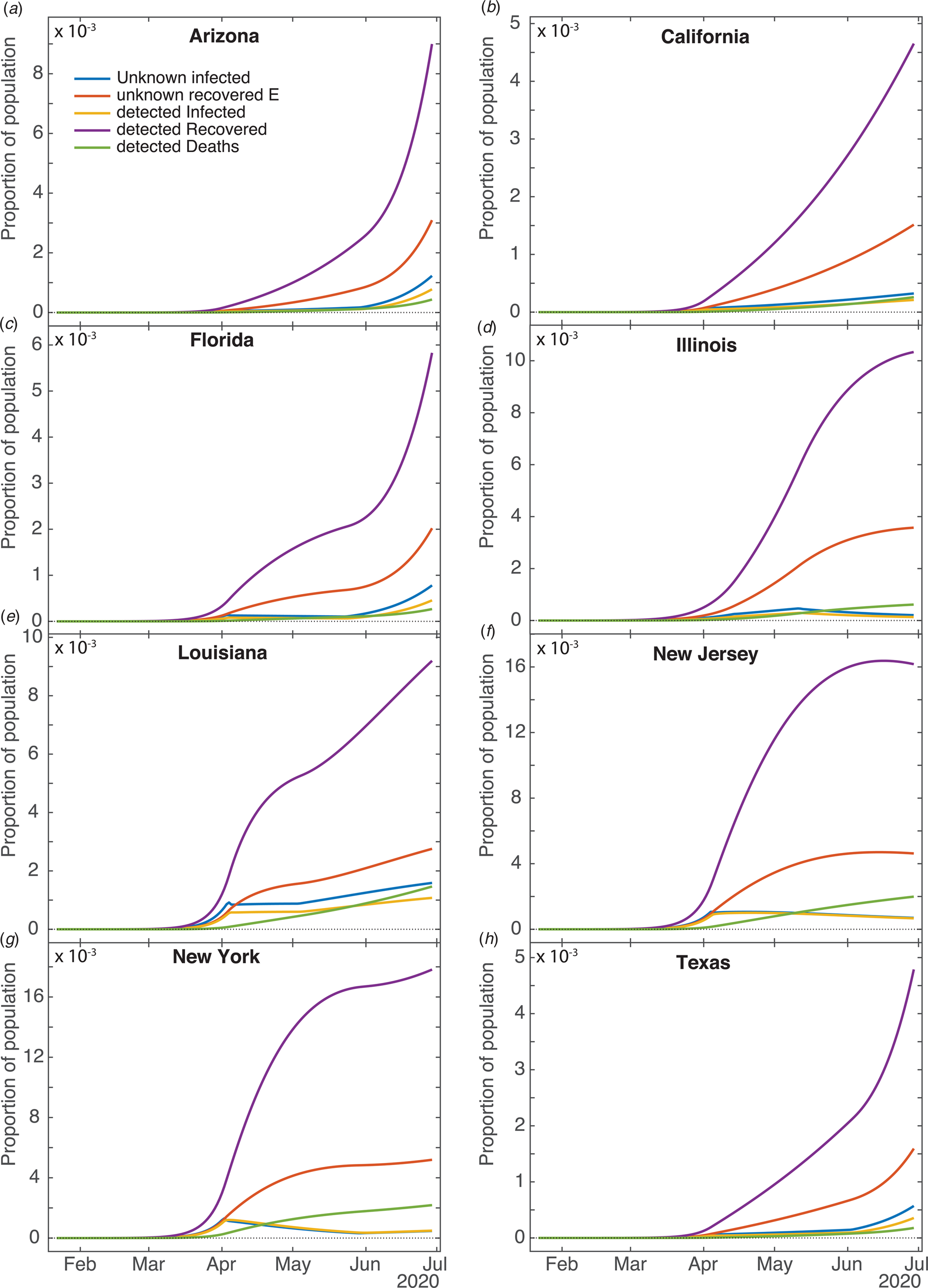
Fig. 3. Computed results for the other compartments for different states. Current unknown infected (U), unknown recovered (E), current detected Infected (I), detected Recovered (R) and detected Deaths (D).
Table 1. SQUIDER model fit parameters for selected US states
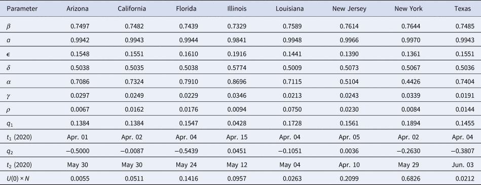
All rate parameters have units of days−1, times have units of days, positive qi values denote to proportions of the S and U compartments, negative q2 values denote to proportions of the Q compartment and the initial condition U 0 × N is given in units of individuals.
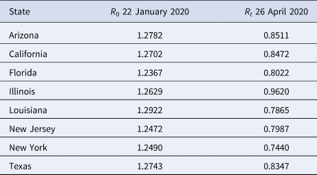
We compare our fit parameters with the classical SIR model which, to remind the reader, involves only Susceptible, Infected and Recovered compartments. The β and parameters correspond to the contact and recovery rates of the SIR model; the fit values imply that for unconstrained epidemic situations (with q(t) = δ = 0) the disease has a reproduction number R 0 = β/ε of around 5. The contact and recovery rates we find are consistent with several prior investigations [Reference Maier and Brockmann17, Reference Liu35]. See Table 2; for further discussion of how the basic SIR model fares in comparison with SQUIDER, see the appendices.
Table 2. Basic R 0 and effective Rt reproduction number values for selected US states
It is surprising that the detection rate δ is so high for all of the states (≈0.5); however, a recent nationwide coronavirus antibody study by the Spanish Health Ministry [Reference Jones36] suggests that the number of unknown infected and unknown recovered in large and heterogeneous jurisdictions, while significant, is not orders of magnitude larger than the number of confirmed cases. This goes against some prior speculation that the asymptomatic and undiagnosed cases might be as much as 10 times the official count [Reference Gaeta37], which would suggest a detection rate 5 times smaller than our δ values.
Returning back to Figure 2 and Table 1, the death rate from diagnosed cases γ falls between around 2% and 3.5%, which is well within the quite wide range of case-fatality rates reported for earlier phases of the pandemic [Reference Roser38]. The recovery rate α for diagnosed cases, seems somewhat high (in the 0.45–0.5 range for New York and New Jersey, and around 0.7–0.8 for the other states); this could reflect the fact that detection of any disease would normally occur after that disease has already partly run its course, but it should be kept in mind as well that this compartment has a minimal effect on the size of the fitted compartments I and D, so the fitting routine may not be as constrained in selecting the α value as the other fit parameters. The re-entry (due to loss of immunity) rate ρ is fairly low for most of the states, which indicates that this is not a significant factor for the initiation of the outbreak. Such low ρ values are not unreasonable since loss of immunity to corona viruses that cause common colds is typically slow, taking several months in some individuals, up to a year in others [Reference Callow23]. Indeed, one recent report found that antibodies in a high proportion of individuals who recovered from Covid-19 started to decrease by about 10% within 2–3 months after infection, suggesting a gradual loss of immunity [Reference Long21]. Surprisingly, Louisiana has a much larger ρ value than other states (≈0.17). This was selected by the fitting routine to account for the unexpected rising new cases during that states' lockdown period. As we see below, the reintroduction of people to the Susceptible compartment obviously results in an endemic infection in the predictions.
Our fitted peak initial sequestration values range over 0.1–0.2 for all states except Illinois (whose value is close to 0.04). The parameter t 1 enables prediction of what day self-isolation policies started having significant effects on case counts – see Table 1. To compare t 1 to states' directives, stay-at-home orders were issued in Arizona on 31 March, California on 19 March, Florida on 1 April, Illinois on 21 March, Louisiana on 23 March, New Jersey on 21 March, New York on 22 March, but was suggested in Texas on 2 April [Reference Mervosh, Lee and Popovich39]. There is a one week or so time lag between announced state action and its measured effect, which may or may not have a physiological basis [Reference Bartels and Achen40]. It is possible that Texas, Arizona and Florida residents were following local orders which prescribed sheltering in place sooner than the state orders: as examples Dallas had a state of emergency declared on 19 March, and Houston residents were urged to stay at home on 24 March [Reference Debenedetto and Watkins41].
Many states partially re-opened in May. Our fit parameter q 2 for the various states corresponds to the percentage of people moving between the Susceptible and Quarantine compartments – where a negative number indicates the percentage decreasing, moving from the Quarantine to the Susceptible compartment. Specifically, Arizona, Florida and Texas had significant numbers (>30%) exiting from stay-at-home conditions, whereas California and Louisiana had smaller numbers (<11%), Illinois had 4.5% additional people enter the Q compartment and New Jersey had a small Q entry (<0.5%). The date at which this occurred, t 2, can also be compared with the dates stay-at-home orders were lifted or expired – also in Table 1. Stay-at-home orders were relaxed or expired on 15 May in Arizona, low-risk businesses and some restaurants opened in California on 8 May; stay-at-home expired in Florida on 4 May, in Louisiana on 15 May, in New York on 28 May, and in Texas on 30 April. New Jersey, on the other hand, did not officially relax social distancing measures within the time range of our data. The time lag between t 2 and official dates may correspond to the end of the school year and people's perception of safety.
The initial values of the undetected infecteds U(0) are all less than one individual (some significantly), implying that none of the states we look at had any actual cases on 22 January (the first day for which we have data). While the ODE results can be scanned to find an estimate for the arrival of the first case (or first two, or five cases) in a jurisdiction, some caution should be exercised in applying this number, since magnitudes at this point are still too small to make statistically valid comparisons. Given that the model estimates there to have been at least 10 cases in the states studied (except Arizona, Florida and Illinois) by the 3rd or 4th week of February (the 1st week of February for New York) we think it is probable that Covid-19 was spreading considerably sooner in New York, New Jersey, Texas and Louisiana than previously assumed. This implies that stronger measures – such as travel bans, cluster identification, contact tracing and quarantine measures – were needed to fully contain the outbreak [Reference Pinotti42, Reference Chinazzi43]. California had reported cases already in late January, yet both the reported data and our ODE model show the main outbreak occurred well after New York or New Jersey. This is likely if the western states were dealing successfully with cases coming directly from Asia, but lost control of the outbreak when infected individuals started arriving from the eastern US or possibly Europe; possible differences between the Asian and European Covid-19 strains are not addressed here.
Model predictions
We have generated predictions using the current fits for two years beyond the first date of recorded US cases. Figure 4a–h show that the total number of infections increases substantially in most states from July 2020 to January 2021, except for Illinois, which apparently experienced its peak case count in May. It is predicted, however, that all states will have continued Covid-19 infections for the next two years, some with small secondary peaks occurring in the spring of 2021. California, Illinois and New Jersey do not have secondary peaks – this is likely due to these states having positive q 2 values (meaning more people enter Q than leave), small negative q 2 values or very small ρ values. Louisiana also does not have secondary peaks – most likely due to this state's large ρ value where reintroduction of sufficient individuals into the susceptible population damps out oscillations in the infected population [Reference Hethcote, Stech and van den Driessche44]. For oscillations to be present in compartment models, cycling of populations has to occur at an intermediate rate – having a high re-entry rate leads to steady infections; and having no re-entry results in eradication of the virus. Our projected daily deaths (Fig. 4i) show that Arizona, Florida, New York and Texas have secondary peaks in deaths after the first main peak. New Jersey and Illinois avoid a secondary peak, presumably because these states haven't yet reopened. We have performed fits to all of the states in the US and predict 11 326 089 cumulative cases, and 8 346 433 cumulative confirmed cases (for all fits R 2 ≥ 0.96), assuming no further interventions (such as additional lockdowns).
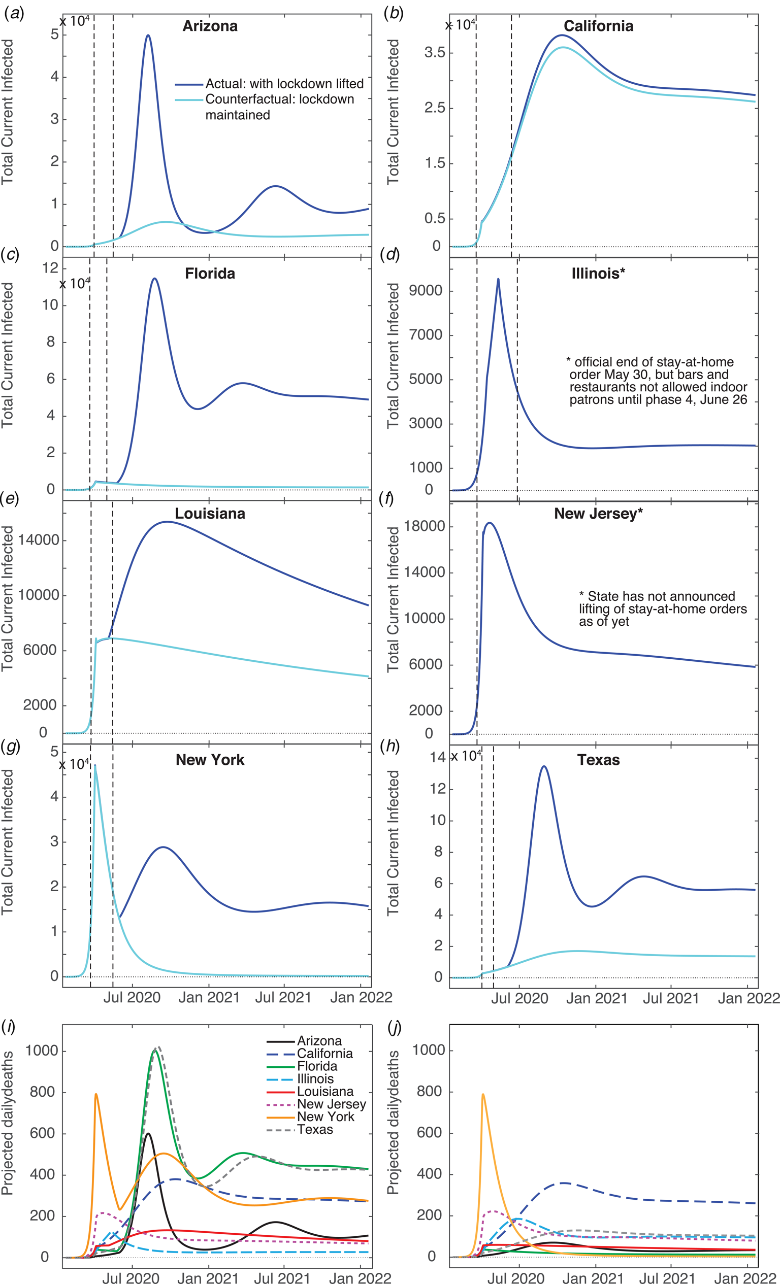
Fig. 4. Model predictions. Total infected (U + I), (I) and confirmed daily deaths (D) for two years beyond the first day of recorded infections generated from our model fits, and the counterfactual scenario of not having lifted stay-at-home orders. The left vertical dashed line indicates the day ‘shelter-in-place’ orders were implemented, and the right vertical dashed line marks the day where such orders were lifted. (I) Confirmed daily death counts for each state for model fits. (J) Confirmed daily death counts for the counterfactual scenario of not lifting orders.
We have also generated counterfactual estimates of case counts (Fig. 4a–h) for the hypothetical situation of sustained stay-at-home orders, i.e. hence disallowing transfer between Q and S. The daily peak total cases is ≈10 times lower for Arizona, Florida, Louisiana, New York and Texas, in comparison with trends predicted from current data. Keeping the stay-at-home orders had weaker effects in Louisiana and California than the other states – due to only releasing small numbers of their Q population back to S (≈10% for Louisiana, <1% for California). Our counterfactual daily deaths (Fig. 4j) show that maintaining staying-at-home could have significantly reduced deaths in Arizona, Florida, Louisiana, New York and Texas. California was not strongly affected because its residents did not fully re-open, and Illinois and New Jersey's counterfactual and factual projections do not differ since these states did not reopen.
Sensitivity to intervention level
Given our grim prediction (Fig. 4), it is natural to ask if there is some non-pharmaceutical intervention (i.e. something other than vaccines) that could improve the situation. We show the effects of actions such as mandating mask-wearing in public by reducing the contact rate β in Figure 5a for Texas. Decreasing β by 10% results in virtual eradication of Covid-19 in Texas within one year. Increasing the detection rate (i.e. test-and-trace) by approximately 15% will also eradicate the virus within a year, shown in Figure 5b, as will also doubling lockdown compliance q 1. These show that β is the most sensitive parameter with respect to reduction of infection rates, though the most practical approach in terms of trade-offs and compliance is simply for governments to increase testing.
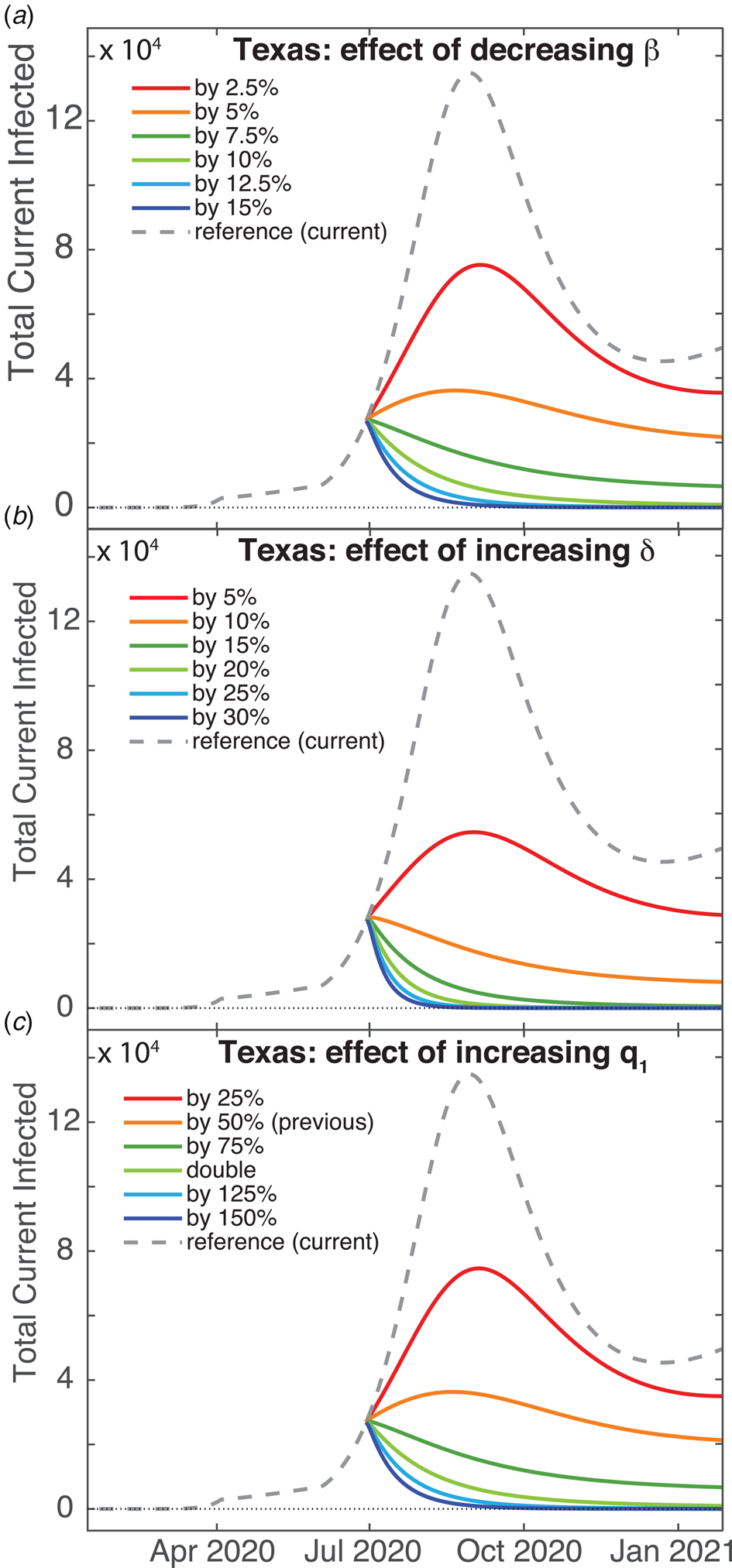
Fig. 5. Predictions for increasing the effect of non-pharmaceutical interventions for Texas. Total (U + I) case counts for: (a) Decreasing the contact rate β, (b) increasing the detection date δ and (c) increasing the sequestration compliance via quarantine rate q 1.
Discussion
Several studies have already modelled the growth of Covid-19 infections and deaths in the US or its various states. As expected for nonlinear systems, some predictions, even if accurate for a short time, can deviate significantly with increased time. A SEIR model (Susceptible, Exposed, Infected, Removed) was implemented on a network to simulate inter-state travel [Reference Peirlinck45]. They predict that, in the absence of countermeasures, the outbreak peaks on day 54 in their simulation (10 May 2020). Other SEIR-type models with additional compartments [Reference Xu15, Reference Moghadas16] including quarantine, also predict that the US outbreak peaks near 10 May 2020 [Reference Xu15], or peaks in the general population 15 weeks into the outbreak (approximately by the last week of April) if only 5% of the population practices self-isolation within a day of symptom onset [Reference Moghadas16]. A logistic model of Covid-19 growth in the US predicts that the cumulative number of cases plateaus by 14 May 2020 [Reference Kriston46]. Alternatively, a neural network parametric model was developed, which predicted that the US would reach the peak number of cases by 8 April 2020 [Reference Uhlig47]. Additionally, a sigmoidal Hill-type model predicts that the US will have 735 920 cases within 76 days of the outbreak, with 41 285 deaths [Reference Aboelkassem48].
More recent Covid-19 models make more dire predictions for the US. A simple SIRD (where D denotes deaths) model [Reference Al-Raeei49], fit to data up to 30 May 2020 predicts that there will be 3.8 million infected and 244 420 deaths by 1 September 2020. A SEIR-type model with additional compartments including unsusceptible (to take into account social distancing), hospitalised and critical populations was proposed by Kennedy et al. [Reference Kennedy26]. They took into account social distancing by removing individuals between the susceptible and unsusceptible compartments at a time-dependent rate. They predict that, for a relaxed social distancing scenario where 40% of the US population is unsusceptible and fitting to data up to 4 May 2020, there will be 60 million infections and 750 000 deaths by December 2020. Li et al. [Reference Li27] have developed a new compartmental model (named DELPHI) based on the SEIR model that also considers additional compartments – undetected, hospitalised and quarantined. Government interventions are taken into account with a time-dependent contact rate. Fitting to data up to 19 May 2020, the model predicts approximately 213 million Covid-19 cases by 15 July 2020, with restrictions on mass gatherings, travel and work.
Zou et al. [Reference Zou50] developed a SEIR model that takes unreported/untested cases into account (named SuEIR). This model, combined with machine learning on data from 22 March to 3 May and data validation between 4 May to 10 May 2020, predicts that Covid-19 infections would have peaked on 1 June 2020, and that there would have been 123 400 total deaths by 30 June 2020. In contrast, after we did our modelling, the IHME Covid-19 Forecasting Team [51] also used a compartmental (SEIR) model with inhomogeneous population mixing (as also ours) to test the impact of non-pharmaceutical interventions on infections and deaths, where changes in population mobility, mask use and social distancing mandates were captured with a time-dependent contact rate. They predict that there will be 430 000 cumulative deaths by 31 December 2020 if social distancing measures are removed, 295 000 deaths if social distancing mandates are imposed when 8 deaths per million residents is surpassed in each state, and 192 000 deaths for a scenario where 95% of the population wears masks and social distancing mandates are imposed at 8 deaths per million. In contrast, our model takes into account all of the critical parameters: undetected infected, possible loss of immunity, sequestration measures, finite detection rates and inhomogeneous mixing between the undetected infected and susceptible populations.
Our model predicts significantly more Covid-19 cases and deaths, with an extended duration past 2 years for the majority of states examined. We aim to extend our predictions to include mask use by incorporating a time-dependent β.
A Covid-19 SEIRS model (where recovered become susceptible again) including co-infection with additional human coronavirus strains and a periodic basic reproduction number R0 corresponding to seasonal forcing, combined with US data, predicts that wintertime outbreaks will occur for several years if immunity wanes – as also occurs with other coronaviruses [Reference Kissler52]. This study also predicts that the number of confirmed Covid-19 cases in the first wave strongly depends on the peak value of R0. Furthermore, social distancing was tested by reducing R0; applied once this may push the epidemic peak to the autumn, whereas intermittent application can reduce the total number of cases [Reference Kissler52].
Delays in transfers between compartments (such as our pseudo-quarantine), and in transferring between several compartments (effectively causing a delay) prior to re-entry in the susceptible population are known to cause oscillations in SIR-type models [Reference Hethcote, Stech and van den Driessche44] – reintroducing individuals into the susceptible compartment de-stabilises the steady rate of infections. Temporary immunity, modelled by our reintroduction of recovered and undetected recovered populations into the susceptible compartment, as well as relaxation of shelter-in-place orders, can produce yearly oscillations such as found in influenza and other human corona viruses (i.e. ‘common colds’) [Reference Callow23, Reference Kyrychko and Blyuss53]. It is possible that without a yearly vaccination program Covid-19 will become endemic in the United States with annual spikes in cases.
In conclusion, we have developed a compartment model taking into account social distancing, undetected infecteds and possible loss of immunity – all issues which are relevant for Covid-19. The model describes current data very well for the states selected for study; this more realistic picture of the disease growth is likely due to both using a larger number of compartments than traditional SIR-type models, and to considering additional nonlinearity in the infectious power of the disease. While projections based on the model are not wholly optimistic, they do point to the fact that it is quite possible to avoid more severe outcomes with stronger measures – increased detection, mask mandates and strict stay-at-home adherence – than have been pursued so far.
Appendices
Methods
All numerical simulation for equations 1–8, fits and data management were done in Matlab. Data for cumulative confirmed cases and deaths were obtained from the Johns Hopkins University (JHU) Center for Systems Science and Engineering, which has been making highly credible US and global Covid-19 time-series statistics available to the public on the GitHub [34] website. Raw data in the original CSV files were converted to Matlab table data structures for ease of access; since the US data were broken out by municipality/county, it was necessary to aggregate this to create each state-wide time series. 2019 estimates of state populations used for normalisation were acquired from the US Census Bureau [54].
Least-squares fits of numerically generated curves to the data were obtained with Matlab's lsqcurvefit using a trust-region-reflective algorithm; this is a variant of the conjugate gradient method designed for large-scale bound-constrained minimisation problems [55]. Hence one of the benefits of this fitting routine is that fit parameters can be given bounds or fixed values (the latter being especially useful during model development and testing). Fit parameters were: all model rate parameters (β, ε, δ, α, γ and ρ), power law exponent a, initial condition for unknown infecteds U(0), plus two pairs of parameters governing sequestration of populations due to social distancing – peak qi values and dates of application ti where i = 1,2. Fits were done in two stages. When work was begun on this project, we had data from 22 January to 9 May, which allowed us to make initial fits for all rate parameters, infectious power, initial conditions and lockdown effects. In the course of writing the results up, we realised we would need to incorporate the effect of breaking developments (cessation of state stay-at-home orders and new spikes in cases), so a second fit was done to determine the time and magnitude of the release of lockdown (q 2, t 2) keeping all of the previous parameter values unchanged.
The algorithm used by lsqcurvefit, like other gradient methods, iteratively navigates through a series of successively better solutions until it finds a local minimum, determined mainly by detection of apparent convergence of the target value (in this case, squared error). Since all the rates are bound between 0 and 1, the ti parameters were rescaled by the total time of the simulation to fall within the same range (this helps the fitting routine when determining step sizes while revising the current solution). Fits were made comparing certain selected and aggregated simulation results against normalised JHU data for cumulative confirmed cases and deaths, simultaneously. lsqcurvefit default values were used for tolerances, iterations and step size, but because the proportions of state populations were so small simulation results and normalised data were rescaled to increase the magnitude of the error, preventing the fit routine from prematurely settling for a solution (the scaling formula was chosen so that the norm of the rescaled test data was equal to the number of elements in the test data matrix).
Simulation results were generated using Matlab's ode45 function, which uses an explicit Runge−Kutta (4, 5) formula. Like almost all numerical ODE solvers, these work iteratively by extending a known value yt to t + Δt by evaluating the derivatives of y at t; RK methods use a sophisticated weighting scheme to correct for the deviations that accumulate using linear extrapolations to estimate a nonlinear function. Default settings were used for the solver, except that the maximum step size was constrained to be ≤ 0.5 days (this prevents the solver, which uses an adaptive step size, from accidentally stepping over the sequestration date t 1). The implementation of the model itself, coded in a function that is given as an argument to ode45, is for the most part straightforward; the only aspect that requires any further comment is the handling of the sequestration function q(t).
As mentioned in the model description, the effect of stay-at-home orders and other social distancing measures is modelled by shifting a segment of the susceptible and unknown infected population into the Q bin, where they cannot be infected or infect others, as the case may be. The interface of ode45 requires that the user supply a subroutine to evaluate the derivatives of the target function at time t, but does not allow direct manipulation of the target function values themselves in mid-run; as well, the user has no way to force the solver to do a derivative evaluation at any particular time. Since the system of ODEs works by transferring populations at various rates between compartments, we resolve these issues by using a timed pulse, i.e. a rate which is generally 0 or close to 0, but which may change any time the solver calls the model subroutine, being relatively large close to the set activation time. For this we use the value of a Gaussian curve at x = t with mean value ti, where the height and width are set so as to achieve the sequestration we desire (easily calculated using Matlab's normpdf function). Since ode45's adaptive step size decreases when it detects unexpected movement in the q rate, a well resolved sampling of different values near the peak ti is obtained. To make analysis more straightforward, we decided that the q i values given to the solver would be equal to the total sequestration effect (e.g. if we set q i to 0.15, then roughly 15% of the S and U compartments would be moved into the Q compartment within a day or two of ti). To achieve this, for sequestrations ≤0.625 we normalised the peak rate to the same value, and set the standard deviation to a value between 0.4 and 0.625 determined by trial and error and fit to a cubic polynomial. For sequestrations above 0.625, a much more complicated formula was needed to achieve the desired effect; since such high sequestration never appeared in any of the fits we will omit any further discussion of this, except to say that to get effective clearance (99.84%) of the entire relevant compartment(s) we use a Gaussian with both height and width set to ≈1.6. See Figure 6 for an example of how the S and Q compartments change over time due to the action of the q pulses.
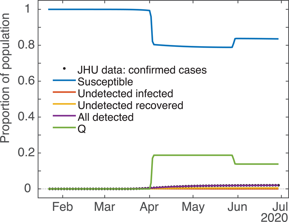
Fig. 6. Computed results for all the compartments (example: New York State). Demonstrating the effect of the ODE model's q pulses timed for 2 April and 29 May on the S (blue) and Q (green) population dynamics. qi values ≈20% and −25%, respectively. Due to the y-axis scale some compartments are partially occluded.
Lastly, for the purpose of doing counterfactual and hypothetical projections, the model implementation subroutine accepts an arbitrary number of peak rate/activation date pairs tacked onto the end of the parameter vector it takes as one of its arguments. This allows us to test the effect of doing several interventions of possibly different magnitudes. Also, a negative peak rate is implemented as returning the specified proportion of the sequestered population in Q back to S (since ode45 has no facility for keeping track of the ratio of S and U populations that were originally sequestered, it was felt that returning everyone to S was the most sensible approach). To make this feasible codewise, at any particular time t only the qi with peak time t ∗i closest to t is executed. In practice, if peaks are set too close to each other (e.g. within half a week or so) they may interfere with each other's ability to achieve full sequestration or release; but since this is essentially the case in real life as well we thought it not to be a priority to address this issue.
The basic SIR model and SQUIDER
As mentioned in the model description, a basic SIR model underlies the SQUIDER model, so the SIR dynamics given the measured contact and recovery rates and estimated initial condition can be computed by setting all other rate parameters to 0 and keeping the power law exponent a = 1. This can be considered a counterfactual case where no interventions of any kind (medical or social) were attempted. Figure 7a compares the result with the empirical cumulative case count. The plotted dynamics show the inevitable SIR dynamics when the basic reproduction number R 0 > 1 (for our New York fit it was ≈5.5), with the S compartment decreasing monotonically from 1 to 0, I compartment peaking, and the R compartment increasing monotonically from 0 to 1.
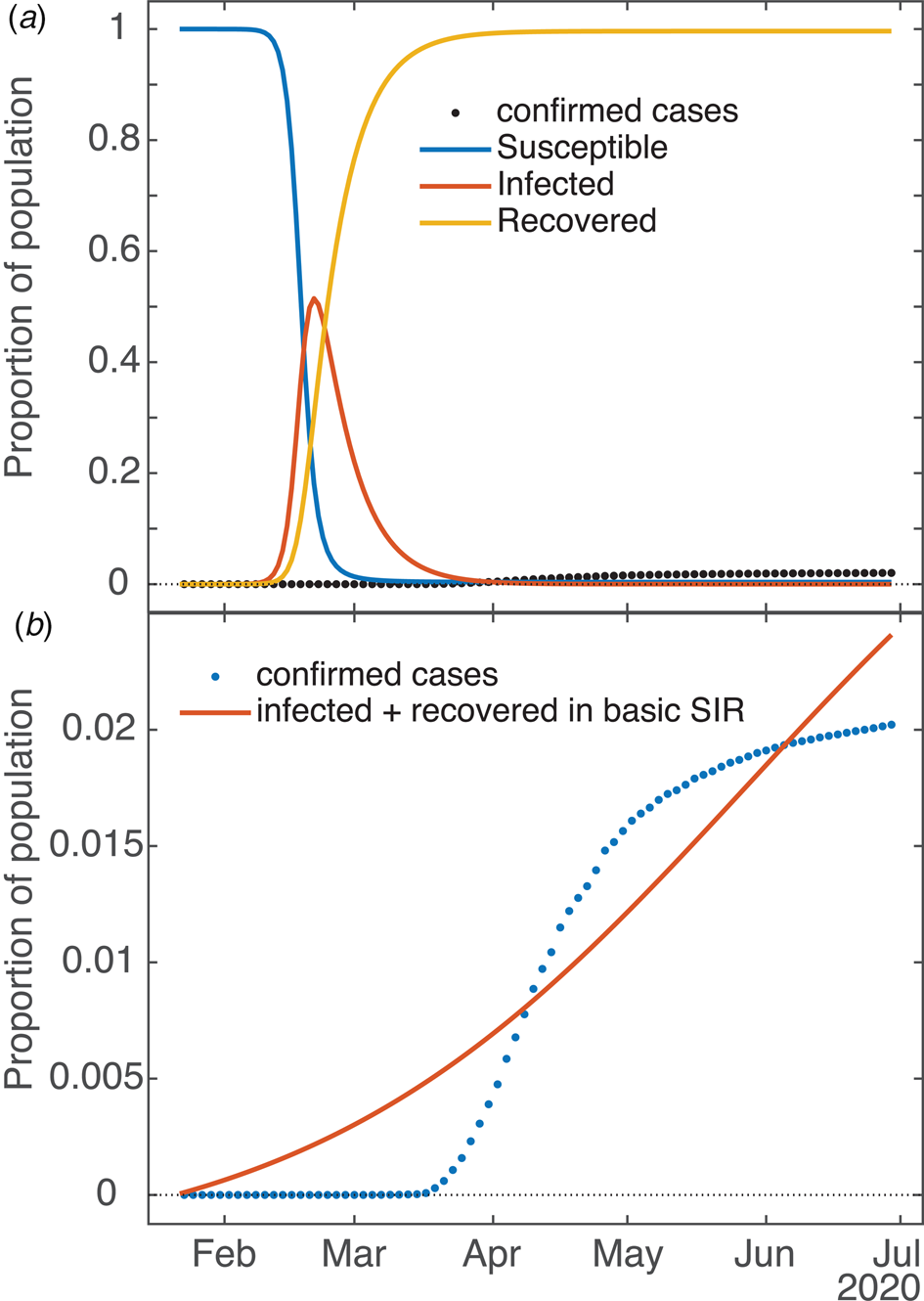
Fig. 7. Applicability of basic SIR model to COVID dynamics (example: New York State). (a) Dynamics of underlying SIR model in SQUIDER fit of NY data (i.e. using only β and values plus initial condition U 0 in the ODE simulation). (b) Attempted independent fit of basic SIR model to empirical data (cumulative cases = combined infected and recovered).
Is it possible to fit the basic SIR model to the available data with good results? Figure 7b shows one such attempt (again, the example is New York). One can see that the fitting routine has placed its relatively uninflected curve between the various inflections of the empirical data (so that, in fact, the signed errors mostly cancel each other), but is incapable of actually capturing the shape. In this case, for the simple SIR model the error measured by the fitting routine (norm of the residuals) was more than 10 times that of the SQUIDER fit to the same data. The R0 for this fit is 1.018, which matches well for the effective R obtained for New York and other states once they started taking measures against the virus (see next section). As mentioned in the previous section, which of the often multiple local minima the fitting routine finds is largely dependent on the starting guess for the parameter set; the one shown is definitely the best of the several attempts we made, but we admit we did not try all possible permutations (nor is it necessary). One work [Reference Al-Raeei49] made predictions using fits of a SIRD model (SIR with a separate Deaths compartment, similar to our detected deaths) to data from various countries. Their fits were obtained by a deterministic method that takes advantage of the fact that the basic SIR ODE model has a closed-form solution. However, the values they obtain for the contact and recovery rates are extremely small (on the order of 10−7), so seem to lose all basis in whatever physical/social meanings the rates have. It should be noted that there are no plots in the paper showing fits against empirical data, and we were not able to make our own since no initial values are given.
The effective reproduction number Rt
In epidemiology, R0 is ‘the basic reproduction number of a disease’ and denotes the expected number of cases produced by a single infected individual in a completely susceptible population. This number, extensively used in epidemiological modelling, describes whether an epidemic breaks out or not; if the value is less than 1 an outbreak does not result in an epidemic, whereas if it is larger than 1 an epidemic occurs [Reference van den Driessche56]. If R0 is much larger than 1, then the outbreak will be stronger and faster. In simple SIR models, it is a direct consequence of, indeed the direct product of three factors: transmissibility (a probability or likelihood of becoming infected), the average number of contacts a person has per day and duration of infectiousness (time to recover, 1/α), namely β/α. Our model is indeed more complex than the traditional, prototypical SIR model (due to its having seven distinct, identified compartments); therefore, the reproduction number R0 necessarily involves additional factors such as q(t), ρ, ε and δ, as well as their initial values (namely at time = 0, the starting point of the modelled epidemic, or of the computational prediction). Since q(t) is time dependent, this necessitates having a time-dependent reproduction number Rt. To compute Rt, we follow the next-generation matrix method [Reference van den Driessche56].
Let x = (x 1,⋅⋅⋅,xn) be the number of individuals in each compartment, where m < n compartments contain infected individuals – here the U and I compartments (i.e. m = 2). Consider the model equations written in the form ${\rm d}x_i/{\rm d}t = {\cal F}_i\lpar x\rpar -{\cal V}_i\lpar x\rpar$ for i = 1,2,…,m. Here ${\cal F}$
 i(x) is the rate of appearance of new infections in compartment i (i.e. positive terms), and ${\cal V}_{\rm i}\lpar x\rpar$
 is the rate of transitions between compartment i and other infected compartments (i.e. negative terms). It is assumed that ${\cal F}$
 i = 0 if i ∈ (m + 1,n); i.e. it is zero for compartments that do not describe infected populations. Define matrices $F = \lsqb {\partial {\cal F}_i\lpar {x\lpar 0 \rpar } \rpar /\partial x_j} \rsqb$
 and $V = \lsqb {\partial {\cal V}_i\lpar {x\lpar 0 \rpar } \rpar /\partial x_j} \rsqb$
 for 1 ≤ i, j ≤ m. Let ψ(0) be the number of infected and undetected infected at the initial time of detection. Then FV −1ψ(0) gives the expected number of new infections; i.e. the matrix FV −1 has the (i,j) item equal to the expected number of secondary infections in compartment i produced by an infected individual introduced in compartment j. Then R0 is given by the largest positive eigenvalue of FV −1. For our model,


which, through taking the product of F and the inverse of V, yields

Note that F and V are 2 × 2 matrixes because we have only two compartments of infected populations – Infected (I) and Undetected infected (U). At the beginning of the outbreak (i.e. t = 0) q(0) = 0, S 0 = S(0) ≈1 and in equation 10 U 0 = U(0) is a fit parameter. Given this form, we can trivially extend equation 10 for later times by including the time dependence of the S, U and q parameters (so that we can get Rt for all times) as

We show R 0 and Rt values on 26 April 2020 – during the sequestration period in many states – in Table 2. Note that while many states face endemic Covid-19 infections (in Fig. 4) despite surprisingly having Rt < 1; this is due to our Rt not taking into account reintroduction of recovered people into the Susceptible compartment, which increases the pool of individuals available for infection.
Acknowledgements
This study was supported by TTU President's Distinguished Chair Funds. We acknowledge early encouragement by Dr Jamilur R. Choudhury to study Covid-19, and humbly dedicate this paper to his memory.
Conflict of interest
None.
Data availability statement
Data for cumulative confirmed cases and deaths were obtained from the Johns Hopkins University (JHU) Center for Systems Science and Engineering, posted on the GitHub website [34].


 Open access