


1. Introduction
Surface engineering using superhydrophobicity is of significant current interest because of its potential for drag reduction and self-cleaning functionality (Rothstein Reference Rothstein2010; Lee, Choi & Kim Reference Lee, Choi and Kim2016). Enhanced slip over these surfaces is caused by the presence of menisci spanning interstitial microstructural grooves or asperities on such surfaces and enclosing gas pockets in the so-called Cassie state. These menisci allow slip and replace an otherwise no-slip zone over which the viscous drag would be larger.
There is growing evidence that these attractive slip properties can be compromised, not only by failure of the Cassie state, but also by the presence of surfactants. Bolognesi, Cottin-Bizonne & Pirat (Reference Bolognesi, Cottin-Bizonne and Pirat2014) used effective slip quantification and imaging of the meniscus shape to argue that superhydrophobic surfaces where the menisci are assumed to be largely free of shear have characteristics suggesting that they are, in fact, closer to being no-slip surfaces. Crowdy (Reference Crowdy2017) confirmed quantitatively that the data of Bolognesi et al. (Reference Bolognesi, Cottin-Bizonne and Pirat2014) are indeed more consistent with immobilization of the menisci, wherein the menisci are taken to be no-slip rather than no-shear. This was done by producing explicit formulae, as a function of downward protrusion angle, groove width and surface pitch, for the effective slip length assuming the menisci are no-slip. Those new formulae were then compared, in both the transverse and longitudinal flow scenarios, with the slip predictions from existing formulae in the literature that take those same menisci to be shear-free (Crowdy Reference Crowdy2017).
Crowdy (Reference Crowdy2017) simply took the surfaces to be no-slip, without specifying any physical reason for it. Bolognesi et al. (Reference Bolognesi, Cottin-Bizonne and Pirat2014), who focused on the longitudinal flow scenario, suggested that surface immobilization might be due to the presence of surface contaminants. With the transverse flow setting in mind, Peaudecerf et al. (Reference Peaudecerf, Landel, Goldstein and Luzzatto-Fegiz2017) have since argued that even trace amounts of surfactants can lead to effective immobilization of a superhydrophobic surface. Models for the slip and drag over such surfaces in the presence of surfactants have since emerged (Landel et al. Reference Landel, Peaudecerf, Temprano-Coleto, Gibou and Goldstein2020). Mayer & Crowdy (Reference Mayer and Crowdy2022) have carried out a numerical study of the immobilization of superhydrophobic surfaces due to the presence of an insoluble surfactant satisfying a nonlinear Langmuir equation of state. Their calculations, which focused on the transverse flow scenario, show that the menisci indeed become immobilized, although the precise cause of it, and the extent of the immobilized meniscus portion, is a delicate function of the surface advection, surface diffusion and surfactant concentration, as well as its intrinsic physical properties.
Baier & Hardt (Reference Baier and Hardt2022) have, however, recently put forward another mechanism by which surfactants can affect a meniscus in the longitudinal flow scenario. They studied the case of a single groove, or trench, of large but finite length spanned by a meniscus contaminated by incompressible surfactant. A model of the flow away from the ends of the trench was produced that is argued to be valid at large Marangoni numbers. The resulting model leads to the result that, in this surfactant-contaminated setting, the meniscus is not a no-slip surface but a surface with constant shear stress determined by the fact that the meniscus is of finite length and the surfactant is incompressible. A prediction of this model is that, at least for the small protrusion angles studied by Baier & Hardt (Reference Baier and Hardt2022), the surface velocities on the meniscus are not zero but, in fact, comprise regions of forward and back flow relative to the main flow direction in the bulk. We refer to these as ‘recirculating flows’ since, when observed from above, they will resemble the surface vortices observed experimentally by Song et al. (Reference Song, Song, Hu, Du, Du, Choi and Rothstein2018). Baier & Hardt (Reference Baier and Hardt2022) point out that the implications of such an effect for hydrodynamic slip are important and remain to be worked out.
That is the subject of the present paper. The interest here is in how the effective slip associated with this constant-shear-stress model differs from one that takes the menisci to be fully immobilized no-slip zones. It is usual to quantify slip for longitudinal shear flow parallel to a periodic array of grooves of infinite length using the hydrodynamic slip length. This is defined to be the quantity  $\lambda$, with the dimensions of length, such that, as $y \to \infty$, the axial flow $(0,0,w(x,y))$ parallel to the grooves in an $(x,y,Z)$ plane has the far-field behaviour $w(x,y) \to \dot {\gamma } (y+\lambda )$, where $\dot {\gamma }$ is the shear rate. An explicit formula for this slip length in this geometry was found by Crowdy (Reference Crowdy2010) when the menisci are assumed to be shear-free and the grooves well spaced relative to their width; this is the ‘dilute limit’ when the no-shear fraction is small. An important feature of the analysis in Crowdy (Reference Crowdy2010) is that the formulae are valid for any protrusion angle of the meniscus. This is a significant point of departure from prior work, where the effect on slip of meniscus curvature was limited to the small-curvature scenario, as in an early important study by Sbragaglia & Prosperetti (Reference Sbragaglia and Prosperetti2007). Indeed, after deriving their model, Baier & Hardt (Reference Baier and Hardt2022) find solutions to it under the same small-protrusion-angle assumption as used by Sbragaglia & Prosperetti (Reference Sbragaglia and Prosperetti2007).
In general conditions, where there is a significant overpressure in the working fluid, there is no reason for this protrusion angle to be small; moreover, even in steady-state flow conditions, this angle must be expected to evolve axially along the flow direction. Indeed, for the different, but closely related, problem of liquid-infused surfaces where the grooves contain a fluid of higher viscosity than the working fluid, the evolution of the protrusion angle of the interface between the two fluids is the important quantity to monitor in order to assess so-called ‘shear-driven failure’ (Wexler, Jacobi & Stone Reference Wexler, Jacobi and Stone2015). Lifting any restriction to small protrusion angles on the solutions of the model of Baier & Hardt (Reference Baier and Hardt2022) is therefore important in extending its range of applicability.
This paper shows that it is possible to find an explicit solution to the single-trench model of Baier & Hardt (Reference Baier and Hardt2022) for any protrusion angle  $\theta$ of the meniscus defined in figure 1(b). This new solution is then used to find a formula, as a function of $\theta$, for the hydrodynamic slip length for longitudinal flow over a dilute periodic array of such trenches, following in the spirit of the clean-flow study of Crowdy (Reference Crowdy2010). When the menisci are free of shear, of width $2c$, Crowdy (Reference Crowdy2010) found the dilute slip length formula
 \begin{equation} \frac{\lambda_{||}^{(no~shear)} }{c}= {\rm \pi}\delta \left (\frac{3 {\rm \pi}^2-4 {\rm \pi}\theta+ 2 \theta^2 }{12 ({\rm \pi}-\theta)^2} \right ), \quad \delta = \frac{c}{L}. \end{equation}
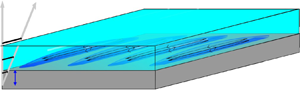
Figure 1. (a) A single trench with a surfactant-contaminated protruding meniscus. (b) The non-dimensional boundary value problem for the longitudinal velocity away from the ends of the trench.
The first new result of this paper is to show that a simple generalization of the analysis of Crowdy (Reference Crowdy2010) gives the dilute slip length when the menisci are no-slip surfaces to be
 \begin{equation} \frac{\lambda_{||}^{(no~slip)} }{c}= {\rm \pi}\delta \left ( \frac{\theta(\theta - 2{\rm \pi}) }{6 ({\rm \pi}-\theta)^2} \right ). \end{equation}
A second result is to show that, for the constant-shear-stress menisci of Baier & Hardt (Reference Baier and Hardt2022), modelling the effect of surfactants, the dilute slip length is
 \begin{align} \frac{\lambda^{surf}_{||} }{c}= {\rm \pi}\delta \left[ \frac{3 {\rm \pi}^2-4 {\rm \pi}\theta+ 2 \theta^2 }{12 ({\rm \pi}-\theta)^2}-{\mathcal{C}}(\theta)\, {\rm{cosec}}\,\theta\,{\int\hskip -1,05em -\,}_{-\infty}^\infty\!(1-\coth{\rm \pi} k\tanh({\rm \pi}-\theta)k)\,{\rm d}k \right], \end{align}
where  $\mathcal {C}(\theta )$, which corresponds to the constant meniscus shear stress value, is determined to be
 \begin{equation} {\mathcal{C}}(\theta) = \frac{ (1-\theta\cot\theta) +{\rm \pi}\displaystyle\ {\int\hskip -1,05em -\,}_{-\infty}^\infty {\rm e}^{({\rm \pi}-\theta) k} {\frac{\sinh\theta k}{\sinh{\rm \pi} k}}(\coth{\rm \pi} k-\tanh({\rm \pi}-\theta)k)\,{\rm d}k}{{\rm \pi}\ \displaystyle{\int\hskip -1,05em -\,}_{-\infty}^\infty {\rm e}^{({\rm \pi}-\theta) k} {\frac{\sinh\theta k}{\sinh{\rm \pi} k}} \frac{1}{k}(1-\coth{\rm \pi} k\tanh({\rm \pi}-\theta)k)\,{\rm d}k }. \end{equation}
Given these explicit formulae, valid in the dilute limit for any protrusion angle, it is then straightforward to compare the slip associated with the different models across the range of flow conditions. Significantly, we find that the slip lengths given by the very different formulae (1.2) and (1.3), and having very different physical origins, are virtually indistinguishable across all protrusion angles. The implications of this result are discussed later.
2. Mathematical formulation
Consider simple shear flow of a Newtonian fluid with viscosity  $\mu$ in the $Z^*$ direction in an $(x^*,y^*,Z^*)$ plane and having shear rate $\dot {\gamma }$. The fluid occupies the upper half $y^*$ plane exterior to a single meniscus, extending infinitely in the $Z^*$ direction, and protruding with angle $\theta$ into the fluid. Outside this meniscus, the rest of the plane $y^*=0$ is a no-slip surface. As for the meniscus itself, this paper examines three different possibilities and compares the effective slip lengths associated with dilute arrays, or ‘mattresses’, of such menisci.
In the model of Baier & Hardt (Reference Baier and Hardt2022), the vapour–fluid interface supports insoluble incompressible surfactant in a high-Marangoni-number and low-Boussinesq-number regime (Manikantan & Squires Reference Manikantan and Squires2020), and essentially reduces to the situation where the meniscus supports a constant, generally non-zero, shear stress. Following Baier & Hardt (Reference Baier and Hardt2022), it is assumed that  $c \ll b$, so that fully developed flow in the groove can be considered, ignoring groove end effects. It is therefore enough to consider a cross-sectional $(x^*,y^*)$ plane that is far enough from the ends of the groove that the flow is well approximated by a unidirectional flow in the $Z^*$ direction, with velocity $(0,0,w^*)$; see figure 1.
Let  ${\mathcal {L}}^*$ denote the no-slip boundary,
 \begin{equation} {\mathcal{L}}^* = \{(x^*,y^*):x^*\in (-\infty,-c] \cup [c,\infty), y^*=0\}, \end{equation}
and let  ${\mathcal {M}}^*$ be the meniscus, forming a circular arc connecting $(\pm c,0)$ with protrusion angle $\theta$ into the fluid, i.e.
 \begin{equation} {\mathcal{M}}^* = \left\{(x^*,y^*)=c\,{\rm{cosec}}\,\theta\,(\cos\phi,\sin\phi-\cos\theta): \phi\in\left(\frac{\rm \pi}{2}-\theta,\frac{\rm \pi}{2}+\theta\right)\right\}. \end{equation}
Mass conservation for the surfactant along  $\mathcal {M}^*$, and far-field shear flow, give rise to the conditions (Baier & Hardt Reference Baier and Hardt2022)
 \begin{equation} w^*=0\quad\text{on}\ \mathcal{L}^*,\quad \int_{\mathcal{M}^*}w^*\,{\rm d}s=0,\quad\frac{\partial w^*}{\partial y^*}\to\dot{\gamma} \quad\text{as }y^*\to\infty. \end{equation}
Dimensionless (unstarred) variables are introduced according to  $(x^*,y^*,Z^*) =c(x,y,Z)$, $w^* = c \dot {\gamma }w$ and $\boldsymbol {n}^*=c\boldsymbol {n}$. The dimensionless model put forward by Baier & Hardt (Reference Baier and Hardt2022) is then
 \begin{equation} \nabla^2 w =0\quad\text{in }D, \end{equation}
with boundary conditions
 \begin{equation} w=0\quad\text{on }\mathcal{L},\quad\frac{\partial w}{\partial n}=C\quad \text{on }\mathcal{M},\quad\frac{\partial w}{\partial y}=1\quad \text{as }y\to\infty, \end{equation}
where  $\boldsymbol {n}$ is the fluid inward normal to $\mathcal {M}$, and the constant $C$ is determined by the condition
 \begin{equation} \int_{\mathcal{M}} w\,{\rm d}s=0.\end{equation}
This last condition describes conservation of surfactant contaminating the meniscus, forced by its incompressible nature combined with the fact that the trenches are of finite length. Readers are referred to Baier & Hardt (Reference Baier and Hardt2022) where this model is described in more detail, and where approximate solutions to it are found for small  $\theta \ll 1$ using a perturbation method. The present paper finds an explicit solution to this model for all $\theta$.
Crowdy (Reference Crowdy2010) found the solution for the flow over a single meniscus in simple shear when the meniscus is taken to be shear-free; he used it to produce formulae (1.1a,b) for the slip length in the dilute limit. (Using a matching procedure, Crowdy (Reference Crowdy2016) later found higher-order approximations in the no-shear fraction, but these will not be used here.) On the other hand, if the menisci are taken to be no-slip surfaces, it turns out that the single-groove problem in this case can be solved by a simple generalization of the analysis of Crowdy (Reference Crowdy2010). Crowdy's analysis of the shear-free case uses a conformal mapping from an upper half-unit disc in a complex  $\zeta$ plane to the fluid region in a complex $z=x+{\rm i}y$ plane and, in terms of that variable viewed as a function of $z$, i.e. $\zeta =\zeta (z)$, Crowdy (Reference Crowdy2010) derives the following expression for the axial fluid velocity $w(x,y)$ in the $Z$ direction:
 \begin{equation} w(x,y) = {\rm Im} \left [ - \frac{{\rm \pi} c }{2 ({\rm \pi}-\theta)} \left (\frac{1 }{\zeta(z)} - \zeta(z) \right ) \right ]. \end{equation}
That same mapping can be repurposed when the meniscus is taken to be a no-slip surface; the only modification is a switch in sign of one of the terms in the analytic function appearing in (2.7), so that the velocity now becomes
 \begin{equation} w(x,y) = {\rm Im} \left [ - \frac{{\rm \pi} c }{2 ({\rm \pi}-\theta)} \left (\frac{1}{\zeta(z)} + \zeta(z) \right ) \right ]. \end{equation}
With this simple change, it is easy to check that the meniscus is now a no-slip zone. Now, the same steps as taken by Crowdy (Reference Crowdy2010) to calculate (1.1a,b) lead to the dilute-limit slip length formula (1.2) for no-slip menisci.
3. Complex variable formulation
The boundary value problem (2.4)–(2.6) can be solved by adapting the conformal mapping methods of Crowdy (Reference Crowdy2010), but here we present a different transform approach. Let
 \begin{equation} w(z,\bar{z})= {\rm Im}[z + f(z)], \end{equation}
where  $f(z)$ is an analytic function in the fluid, decaying in the far field, satisfying
 \begin{equation} {\rm Im}[\,f(z)]=0\quad\text{on }\mathcal{L},\quad \frac{\partial}{\partial n}{\rm Im}[z+f(z)]=C\quad \text{on }\mathcal{M}. \end{equation}
Simple geometrical arguments reveal that the meniscus lies on a circle of radius  $r={\rm cosec}\,\theta$ centred at complex location $z_0=-{\rm i} \cot \theta$. With $s$ denoting arclength along the meniscus (increasing with fluid to the left), the Cauchy–Riemann equations imply that, on $\mathcal {M}$,
 \begin{equation} \frac{\partial}{\partial n}{\rm Im}[z+f(z)] = \frac{\partial}{\partial s}{\rm Re}[z+f(z)]=C. \end{equation}
On integration on  $\mathcal {M}$, using ${\rm d}s =-r \,{\rm d}\phi$, where $\phi ={\rm arg}[z-z_0] = -{\rm Re}[{\rm i}\log (z-z_0)]$, one obtains
 \begin{align} {\rm Re}[z+f(z)] ={-} Cr \phi + c_0 &= C r \,{\rm Re}[{\rm i}\log(z-z_0)] + c_0 \nonumber\\ & = C \,{\rm cosec}\,\theta\,{\rm Re} \left[{\rm i}\log(\cot\theta-{\rm i} z)\right], \end{align}
where a convenient choice of the integration constant  $c_0$ has been made. The challenge now is to find $f(z)$, with ${\rm Im}[\,f(z)] \to 0 \text { as }y\to \infty$, satisfying
 \begin{equation} {\rm Im}[\,f(z)] = 0 \quad\text{on }\mathcal{L}, \quad {\rm Re}[\,f(z)] ={-}{\rm Re}[z]+C\,{\rm cosec}\,\theta\,{\rm Re} [{\rm i}\log(\cot\theta-{\rm i} z)] \quad \text{on }\mathcal{M}. \end{equation}
Now introduce
 \begin{equation} z = Z(\eta) = \tanh\frac{\eta}{2}, \quad\eta = Z^{{-}1}(z) = \log\frac{1+z}{1-z}, \end{equation}
which are conformal mappings between  $D$ and a horizontal strip domain in a complex $\eta$ plane. The point at infinity in the $z$ plane is mapped to $\eta ={\rm i}{\rm \pi}$ in the $\eta$ plane; the edge points $z = \pm 1$ are transplanted to the two ends of the infinite strip in the $\eta$ plane. The boundaries $\mathcal {L}$ and $\mathcal {M}$ correspond to infinite horizontal lines in the $\eta$ plane:
 \begin{equation} \mathcal{M} \mapsto \varGamma := \{\eta:{\rm Im}[\eta]=\theta\}, \quad \mathcal{L} \mapsto \varSigma := \{\eta:{\rm Im}[\eta]={\rm \pi}\}. \end{equation}
 Now define the composed function  $H(\eta ):=f(Z(\eta ))$ which, by composition of analytic functions, is an analytic function of $\eta$ in the strip image of $D$. The boundary conditions are
 \begin{gather} H(\eta)-\overline{H(\eta)}=0 \quad\text{on } {\varSigma}, \end{gather}
 \begin{gather}\frac{1}{2}\left(H(\eta)+\overline{H(\eta)}\right) ={-}{\rm Re}\left[\tanh\frac{\eta}{2}\right]+C\,{\rm cosec}\,\theta\, {\rm Re}\left[{\rm i}\log\left(\cot\theta-{\rm i} \tanh\frac{\eta}{2}\right)\right]\quad\text{on }\varGamma. \end{gather}
Finding  $H(\eta )$ is now possible by modifying a transform method in a strip used by Crowdy & Davis (Reference Crowdy and Davis2013) and Crowdy & Brzezicki (Reference Crowdy and Brzezicki2017) in different contexts. First, introduce the transform functions of a complex variable $k$:
$k$:
 \begin{equation} \rho_1(k)=\int_{-\infty + {\rm i} \theta}^{\infty+{\rm i} \theta} H(\eta){\rm e}^{-{\rm i} k\eta}\,{\rm d}\eta, \quad \rho_2(k)={-}\int_{-\infty + {\rm i} {\rm \pi}}^{\infty+{\rm i} {\rm \pi}} H(\eta){\rm e}^{-{\rm i} k\eta}\,{\rm d}\eta. \end{equation}
These two functions depend on  $\theta$, but this dependence is suppressed in our notation. Relations between these functions can be obtained by multiplying the boundary conditions (3.7a,b) and (3.9) by ${\rm e}^{-{\rm i} k\eta }$ and integrating along the respective boundaries:
 \begin{align} \left.\begin{gathered} \rho_2(k)-{\rm e}^{2k{\rm \pi}}\overline{\rho_2({-}k)}=0, \\ \frac{1}{2}\left(\rho_1(k)+{\rm e}^{2k\theta}\overline{\rho_1({-}k)}\right)=\frac{{\rm \pi}{\rm i}}{\sinh{\rm \pi} k}(1+{\rm e}^{2k\theta})+C \,{\rm cosec}\,\theta\frac{{\rm \pi}{\rm i}}{k\sinh{\rm \pi} k}(1-{\rm e}^{2k\theta}). \end{gathered}\right\} \end{align}
There is a so-called ‘global relation’ (Crowdy & Davis Reference Crowdy and Davis2013; Crowdy & Brzezicki Reference Crowdy and Brzezicki2017) relating these functions:  $\rho _1(k)=-\rho _2(k):=\rho (k)$ for $k\in \mathbb {R}$. Combining this with the boundary conditions (3.11) allows, after some algebra, for $\rho (k)$ to be found explicitly as
 \begin{align} \rho(k) =2{\rm \pi}{\rm i} {\rm e}^{{\rm \pi} k}\left(\coth{\rm \pi} k-\tanh({\rm \pi}-\theta)k-\frac{C\,{\rm cosec}\,\theta}{k}(1-\coth{\rm \pi} k\tanh({\rm \pi}-\theta)k)\right). \end{align}
The inverse transform is furnished (Crowdy & Davis Reference Crowdy and Davis2013; Crowdy & Brzezicki Reference Crowdy and Brzezicki2017) by
 \begin{equation} H(\eta) = \frac{1}{2{\rm \pi}} \, {\int\hskip -1,05em -\,}_{-\infty}^\infty\rho(k){\rm e}^{{\rm i} k\eta}\,{\rm d}k, \end{equation}
where  ${\int\hskip -1,05em -\,}$ denotes a principal value integral.
Consequently, an explicit solution for the flow is
 \begin{equation} w(z,\bar{z}) ={\rm Im}\left[z+\frac{1}{2{\rm \pi}}\,{\int\hskip -1,05em -\,}_{-\infty}^\infty\rho(k){\rm e}^{{\rm i} k\eta(z)}\,{\rm d}k\right]= w_0(z,\bar{z})-C\,{\rm cosec}\,\theta \, w_1(z,\bar{z}), \end{equation}
where
 \begin{gather} w_0(z,\bar{z})= {\rm Im} \left[-\frac{2{\rm \pi}}{{\rm \pi}-\theta} \frac{(z^2-1)^{{\rm \pi}/(2({\rm \pi}-\theta))}}{(z-1)^{{\rm \pi}/({{\rm \pi}-\theta})}- (z+1)^{{\rm \pi}/({{\rm \pi}-\theta})}}\right], \end{gather}
 \begin{gather}w_1(z,\bar{z}) ={\rm Im}\left[\,{\int\hskip -1,05em -\,}_{-\infty}^\infty \left(\frac{1+z}{1-z}\right)^{{\rm i} k} \frac{{\rm i} {\rm e}^{{\rm \pi} k}}{k}(1-\coth{\rm \pi} k\tanh({\rm \pi}-\theta)k)\,{\rm d}k\right], \end{gather}
with  $w_0(z,\bar {z})$, whose inverse transform can be found analytically, retrieving the zero-shear-stress result (1.1a,b) of Crowdy (Reference Crowdy2010). Condition (2.6) now gives $C$ as a function of $\theta$ as
 \begin{equation} C = \mathcal{C}(\theta)=\sin\theta\frac{\displaystyle\int_{\mathcal{M}}w_0(z,\bar{z}) \,{\rm d}s}{\displaystyle\int_{\mathcal{M}}w_1(z,\bar{z})\,{\rm d}s}, \end{equation}
which, after evaluation of the integrals, yields the earlier reported (1.4). For  $\theta \ll 1$, this formula reproduces $C$ as found by Baier & Hardt (Reference Baier and Hardt2022), as shown in figure 2.

Figure 2. Graph of  $\mathcal {C}(\theta )$ against $\theta$. The dashed line shows the small-angle results of Baier & Hardt (Reference Baier and Hardt2022).
Figure 3 depicts the contours of constant axial velocity for these solutions for a range of protrusion angles (by symmetry, only plotting half of the physical domain). These match with the plots given by Baier & Hardt (Reference Baier and Hardt2022) but extend them to menisci with larger protrusion angles. Similarly, figure 4(a) replicates their results for the velocity along the meniscus for small protrusion angles, with figure 4(b) extending these to larger angles. The flow reversal on the meniscus, which is necessary to maintain conservation of surfactant, manifests differently for menisci that protrude into or out of the flow: that is, with flow reversing at the tips of the meniscus in the former case, and at the centre of the meniscus in the latter. Figure 4 adds to this understanding, illustrating that, for larger protrusion angles, a smaller proportion of the meniscus experiences flow reversal near the meniscus edges.

Figure 3. Velocity contours for (a)  $\theta =0.2$, (b) $\theta =0.6$, (c) $\theta =-0.2$, (d) $\theta =1.2$ and (e) $\theta =-1.2$. Panels (a)–(c) retrieve figures 3(a), 3(c) and 3(d), respectively, of Baier & Hardt (Reference Baier and Hardt2022). The dotted contour corresponds to $w=0$.

Figure 4. Velocity along the meniscus,  $w|_{\mathcal {M}}$, plotted against $x$. Panel (a) replicates figure 4(a) in Baier & Hardt (Reference Baier and Hardt2022), while panel (b) extends this to menisci with larger protrusion angles. Note that the graphs are multivalued for $\theta >{{\rm \pi} }/{2}$, as the meniscus ‘bulges’ so much that it hangs over the adjacent edge of the no-slip surface.
4. Hydrodynamic slip length
Given this explicit solution, its far-field behaviour, and consequently the effective slip length, can be extracted. Note that
 \begin{equation} w(z,\bar{z}) \sim {\rm Im}\left[z +\frac{\varLambda(\theta)}{z}+O\left(\frac{1}{z^2}\right) \right] \quad \text{as }y\to\infty, \end{equation}
where
 \begin{equation} \varLambda(\theta) = \frac{{\rm i}}{\rm \pi}\,{\int\hskip -1,05em -\,}_{-\infty}^\infty k{\rm e}^{-{\rm \pi} k}\rho(k)\,{\rm d}k, \end{equation}
which is a real function of  $\theta$. Consider the single groove depicted in figure 1 now repeated periodically with period $2L$ in the $x$ direction and let $\delta ={c}/{L}$; this is the meniscus fraction per period. For $\delta \ll 1$ (Crowdy Reference Crowdy2010, Reference Crowdy2016) the flow is well approximated as a linear superposition of the effect of each groove, namely,
 \begin{equation} \hat{w}(z,\bar{z})\sim{\rm Im}\left[z+\varLambda\sum_{n={-}\infty}^{\infty}\frac{1}{z-2n/\delta}+O\left(\frac{1}{z^2}\right)\right]. \end{equation}
Referring to the identity
 \begin{equation} \sum_{n={-}\infty}^{\infty}\frac{1}{z-2n/\delta} = \frac{\delta{\rm \pi}}{2}\cot\frac{\delta{\rm \pi} z}{2}\to-\frac{{\rm i}\delta{\rm \pi}}{2}\quad\text{as }y\to\infty, \end{equation}
and returning to dimensional variables, we infer
 \begin{equation} \hat{w}^*(x^*,y^*)\sim \dot \gamma \left(y^*-\frac{c^2\varLambda(\theta) {\rm \pi}}{2L}\right)\quad \text{as }y^*\to\infty, \end{equation}
leading to the slip length formula (1.3).
Figure 5 is the most important graph of this paper. It shows that both the no-slip model and the constant-shear-stress model dramatically compromise slip compared to the shear-free result of Crowdy (Reference Crowdy2010). But it also shows that the effective slip lengths associated with the former two very distinct models are virtually indistinguishable across the whole range of protrusion angles, i.e. across all operating conditions. Intuitively, the separate regions of forward and reverse recirculating flow on the meniscus forced by the incompressibility condition (2.6) cause flows in the bulk that ‘average out’ in the far field to produce an effective slip length close to that where the meniscus is completely immobile. A practical ramification of this observation is that, for the constant-shear-stress model, the much simpler formula (1.2) can be used as a good approximation in lieu of the more complicated (but still explicit) result (1.3). It is also known (Kirk Reference Kirk2018) that the slip lengths associated with semi-infinite shear flow provide excellent estimates of the effective slip in channel flows, rendering the new formulae of this paper of broader significance. Finally, in principle, the same transform methods used above are likely to produce higher-order formulae in  $\delta$ in the spirit of Crowdy (Reference Crowdy2016), but these corrections are not expected to affect the trend of the observations just made in the dilute limit.

Figure 5. Normalized effective slip length,  $\lambda /(\delta c)$, as a function of $\theta$ assuming no-shear menisci following Crowdy (Reference Crowdy2010), no-slip menisci and constant-shear-stress menisci. The last two remain close across the range of protrusion angles.
Lee et al. (Reference Lee, Choi and Kim2016) have commented that ‘the widely inconsistent quantitative results in the literature have led to some fundamental misunderstandings and false anticipations’, and the results of this paper underscore the need for caution in interpreting experimental data, especially when measuring effective slip and comparing to theoretical models (Manikantan & Squires Reference Manikantan and Squires2020). It has been demonstrated here, using exact solutions of two distinct theoretical models, that the effective slip lengths associated with longitudinal flow over a dilute mattress of trenches assuming fully immobilized menisci are almost identical to the slip lengths if those menisci are, in fact, mobile constant-shear-stress surfaces exhibiting non-trivial recirculating flow patterns caused by mass conservation of contaminating surfactants.
Conflict of interests
The authors report no conflict of interests.


 Open access